Sage Journals: Discover world-class research

Abstract

Predicting indoor airflow distribution in multi-storey residential buildings is essential for designing energy-efficient natural ventilation systems. The indoor environment significantly impacts human health and well-being, considering the substantial time spent indoors and the potential health and safety risks faced daily. To ensure occupants’ thermal comfort and indoor air quality, airflow simulations in the built environment must be efficient and precise. This study proposes a novel approach combining Computational Fluid Dynamics (CFD) simulations with machine learning techniques to predict indoor airflow. Specifically, we investigate the viability of employing a Deep Neural Network (DNN) model for accurately forecasting indoor airflow dispersion. The quantitative results reveal the DNN’s ability to faithfully reproduce indoor airflow patterns and temperature distributions. Furthermore, DNN approaches to investigate indoor airflow in the residential building achieved an 80% reduction in the time required to anticipate testing scenarios compared with CFD simulation, underscoring the potential for efficient indoor airflow prediction. This research underscores the feasibility and effectiveness of a data-driven approach, enabling swift and accurate indoor airflow predictions in naturally ventilated residential buildings. Such predictive models hold significant promise for optimizing indoor air quality, thermal comfort, and energy efficiency, thereby contributing to sustainable building design and operation.

Keywords

Computational fluid dynamics (CFD)machine learning deep neural network (DNN)indoor airflow prediction natural ventilation building environment

Introduction

Nowadays, people spend 80%–90% of their time in buildings (Hajdukiewicz et al., 2013; Jamaludin et al., 2014; Shaikh et al., 2013). Since the early 21st century, the issues about indoor air quality, natural ventilation systems, and occupants’ health in common indoor spaces have more interest in infectious airborne virus risks in buildings such as Severe Acute Respiratory Syndrome-2003, Middle East Respiratory Syndrome-2012, and Coronavirus Disease-2019. In addition, comfort in the built environment is essential for human health and increases work productivity. One of the vital tasks in intelligent buildings is maintaining an acceptable interior thermal environment because the thermal environment significantly impacts inhabitants’ health, productivity, and working efficiency (Chen et al., 2020, 2021; Chenari et al., 2016; Costa et al., 2013; Huang & Liao, 2022; Park & Chang, 2020; Yang & Wang, 2012). Natural ventilation uses natural forces such as wind-driven force and buoyancy-driven force, as well as wind direction, to supply and remove air from the outside to the inside (Tominaga & Blocken, 2015), with the potential to save 30%–40% on energy usage compared to mechanical ventilation systems (Gratia & De Herde, 2004; Kolokotroni & Aronis, 1999; Schulze & Eicker, 2013). Natural ventilation is a trend for sustainable development for facilities to improve energy consumption, thermal comfort, and a healthy indoor environment. Natural ventilation can enhance indoor and outdoor air exchange and provide occupants with internal air renewal and thermal comfort, especially in traditional residential buildings. Sick building syndrome (SBS) is easy to develop when a building does not have enough ventilation (Al-qahtani, 1993; Common, 2003; Klepeis et al., 2001; Wargocki et al., 2002). Research on natural ventilation strategies in buildings in Singapore has represented that whole-day ventilation can enhance thermal comfort in hot-humid climates (Liping & Hien, 2007). A natural ventilation system can help to improve thermal comfort in the building. Still, the effectiveness of natural ventilation depends on the climate condition, and the authors gave that manual window opening control as an alternative to achieve thermal comfort in the building (Raja et al., 2001).

The computational fluid dynamics (CFD) technique has recently become more familiar in forecasting natural ventilation performance as computing capability has advanced (Cook et al., 2003; Cook & Lomas, 1998; Liu et al., 2009, 2015, 2018; Nielsen, 2015; Qi & Wei, 2020; Yazarlou & Barzkar, 2022; Zhai, 2006; Zhang et al., 2022). Wind-driven CFD tests have demonstrated that the passive technique can meet thermal comfort while enhancing air velocity by reducing indoor temperatures and energy consumption (Elshafei et al., 2017; Hong et al., 2017; Raji et al., 2020). The use of CFD to study thermal comfort conditions in buildings has been investigated (Blocken, 2015; Deng & Tan, 2019; Elshafei et al., 2017; Hong et al., 2017; Raji et al., 2020). Building energy modeling is another way to assist innovators in designing and developing building system concepts, such as displacement ventilation, under various dynamic operating situations. However, this technique is widely considered to limit spatial resolution for performance prediction of stratified indoor settings (Chen, 2009; Vladimir, 1967). Full-scale measurements can enable researchers to investigate real-world events’ complexities. However, it is often impractical to make measurements at all places in the domain and control all boundary conditions in full-scale experiments (Blocken, 2014; Chen, 2009; Tominaga et al., 2008).

ML algorithms have brought significant advancements in various fields, from initial perception to deep learning models (Courville, 2016). Leveraging artificial intelligence (AI), such as Deep Neural Networks (DNNs), for airflow prediction shows promise as an alternative to CFD analysis in the future (Guo et al., 2016; Umetani & Bickel, 2018). Unlike CFD, which relies on wind tunnel test data, DNNs offer the advantage of swiftly deriving wind velocity distributions based solely on input conditions of various structures within the target area. Consequently, this approach significantly reduces computation time, enabling parametric studies, short-time optimization calculations, and various other applications. In recent trends, practical research on accuracy validation has emerged in different domains, including meteorology and wind power generation prediction (Harbola & Coors, 2019; Huang & Kuo, 2018; Zhou et al., 2018). While ongoing efforts seek to enhance CFD techniques through novel algorithms and turbulence models (Berger et al., 2005; Spalart & Garbaruk, 2021), there has recently been a surge of interest in new tools to replace CFD in the analysis of fluid mechanics problems, typically for faster predictions or as an aid to the CFD simulation for improved accuracy. AI and data-driven models are gaining popularity in applications with digitalization and large amounts of data. In particular, deep learning and DNN are particularly intriguing in terms of their skills as universal nonlinear approximates, large dimensionality fields, and computational inexpensiveness. Several studies have replaced CFD simulations with deep learning methods, using DNNs as surrogate models for numerical simulations. Depending on the situation, Surrogate modeling can enable magnitudes quicker airflow prediction (Tanaka et al., 2019), and even real-time forecasts addressing one of the two issues mentioned by CFD simulations (Hintea et al., 2015). As a result, DNN models, with their superior modeling capabilities and high-speed computing prowess, emerge as viable alternatives for airflow prediction in naturally ventilated residential buildings.

In indoor airflow prediction in naturally ventilated residential buildings, while CFD simulations can provide valuable insights into realistic wind patterns indoors and outdoors, their setup demands considerable technical expertise. Additionally, addressing numerical problems and hardware requirements for processing time can lead to substantial expenses. In the past, researchers have developed outdoor wind velocity ratio prediction models to anticipate outdoor ventilation possibilities on an urban scale, enabling faster decision-making during the early design phase. However, existing prediction models often fall short: linear regressions fail to adequately explain high-density urban airflow and nonlinear regressions with predefined equation forms present significant barriers for urban planners and architects due to their reliance on extensive technical expertise. To address these challenges, a more sophisticated data-driven machine learning approach emerges as a promising solution. This approach makes it possible to train nonlinear regression models without predefined equation formats, making it more accessible and adaptable for users. Table 1 shows the research that couples the CFD and machine learning approaches.

Table 1.

Summary of existing studies using DL models and CFD in a built environment.

References	DL models	CFD turbulence model	Configuration	Purpose of work	Research gap
Zhou and Ooka (2021a)	NN	RANS k − ε	2D-room	This study focuses on developing a fast and accurate prediction model for internal airflow patterns and temperature distributions using a neural network (NN). The NN model is trained, validated, and tested using the CFD database.	The research gap in this paper is the need for a more comprehensive investigation into the selection and customization of preprocessing methods for neural networks in indoor environment prediction and the potential extension of the study to address complex three-dimensional scenarios and other factors affecting indoor air quality and thermal comfort.
Zhou and Ooka (2021b)	NN	RANS k − ε	3D-room	This study aims to validate the viability of NN for fast and accurate indoor airflow prediction by extending previous experiments from 2D to 3D indoor environments, thus providing more realistic settings.	The limitations of this paper include a relatively small and possibly non-representative testing dataset, sensitivity to hyperparameters, and the absence of in-depth exploration of real-world applications and robustness to noisy data.
Zhou and Ooka (2022)	NN	Laminar calculation	Test room	This study introduces a novel linked simulation framework for rapid building energy simulation, considering the non-uniform indoor climate. The framework integrates a NN model with a Modelica-based energy simulation tool, enabling quick prediction of indoor air distribution.	The limitations of this paper include limited testing cases, potential hyperparameter sensitivity, challenges related to the assumption of linear superposition, the complexity of data synchronization, lack of real-time application testing, limited real-world validation, dependency on training data quality, potential hardware and software dependencies, and a lack of comprehensive comparisons with other surrogate models or methods.
Tian et al. (2022)	BP (ANN)	RNG k − ε	Typical consultation room	This study aims to predict indoor environment indicators at different elevations, intending to provide healthy stratified environments using data from traditional building management systems. Additionally, the study considers cooling and heating conditions in a consulting room with lateral air intake.	The limitations of this paper include reliance on ANN models, which may not capture all complex factors in stratified indoor environments, potential oversimplification of inputs and assumptions (e.g. using only air supply and exhaust temperatures), a focus on prediction rather than system optimization, and a lack of exploration of other data-driven models or comparison with alternative methods for predicting indoor environment indicators.
Cheng et al. (2022)	GA, KNN	N/A	Commercial building	This article showcases the deployment of sensors for thermal comfort and indoor air quality using Building Information Modeling (BIM), CFD, and Genetic Algorithm (GA). The study develops a general procedure for fitting sensors that measure temperature and CO₂, which is critical to ensuring thermal comfort and indoor air quality.	The limitations of this paper include simplified occupant representations, the exclusion of insulation effects, steady-state simulations, limited consideration of tenant areas, a focus on CO₂ and temperature, a single optimization algorithm, limited generalizability, unverified assumptions about MVAC systems, a narrow scope of scenarios and parameters, a lack of field validation, and the need for further exploration of various pollutants and machine learning algorithms.
Gheziel et al. (2022)	ANN	Standard k − ε model	a scaled test chamber	The ANN model in this study is developed through network learning using an experimental database. Its primary objective is to achieve a more precise indoor particle concentration distribution smoothing. The ANN model is compared to the CFD approach, employing identical assumptions and flow regimes to assess its performance.	The limitations of this paper include a reliance on an artificial neural network model without extensive experimental validation, a narrow focus on fine particle distribution, and a simplified representation of indoor air quality parameters and geometry.
Zhou and Ooka (2020)	DNNs	RANS k − ε	2D office room	This work aims to investigate the viability of DNN in quickly and accurately predicting indoor airflow distribution using a two-dimensional isothermal example. DNN is employed to predict isothermal air flows based on a CFD database. The performance of the DNN model on predictions of training instances and test cases is compared to study the influence of DNN architecture.	The limitations of this paper include its reliance on simplified CFD simulations without experimental validation, a narrow focus on specific DNN architectures, sensitivity to input ranges and resolutions, and the omission of real-world complexities, potentially limiting its generalizability and practical application.
Warey et al. (2020)	LRWSGD, RF, ANN	RANS k − ε	The vehicle cabin	In this study, a data-driven tool is developed utilizing high-fidelity CFD simulations and machine learning algorithms. The device predicts occupant thermal comfort for various combinations of glazing grades, environmental conditions, and HVAC settings on each window surface.	The limitations of this paper include potential software-specific biases in modeling, the absence of validation against real-world vehicle data, neglect of transient conditions, and the inability to account for individual passenger comfort preferences.

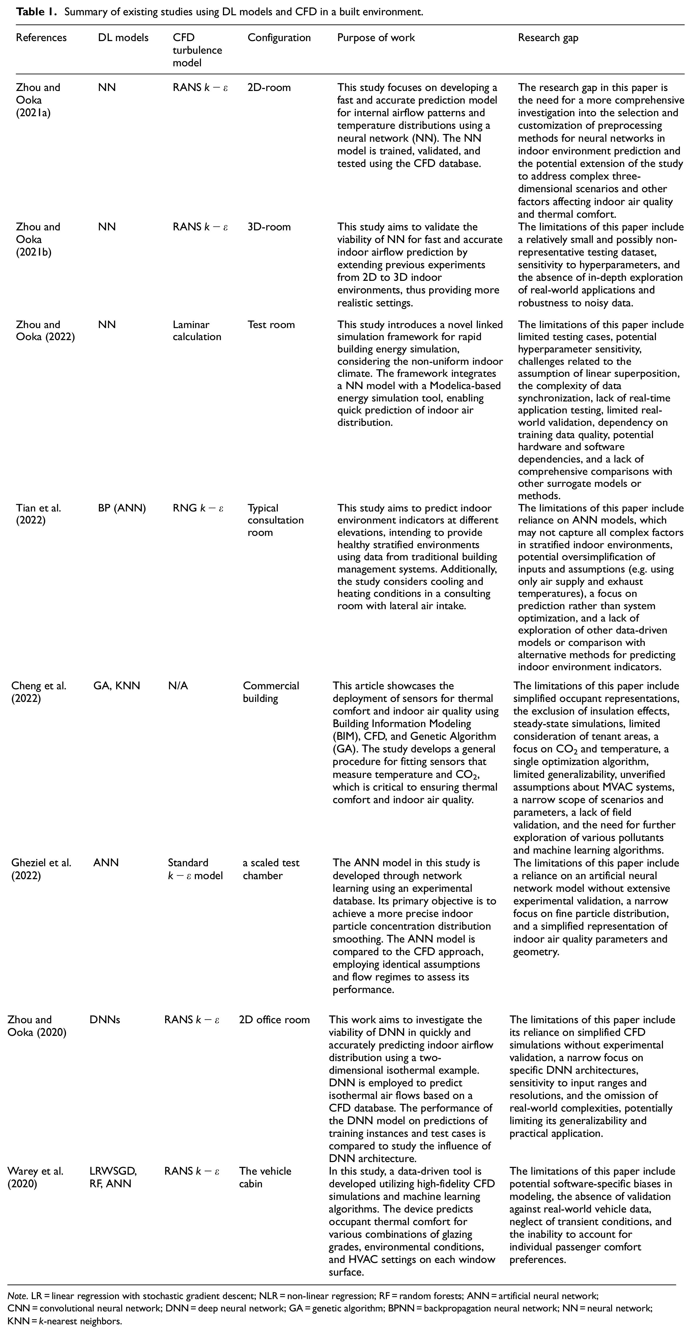
Note. LR = linear regression with stochastic gradient descent; NLR = non-linear regression; RF = random forests; ANN = artificial neural network; CNN = convolutional neural network; DNN = deep neural network; GA = genetic algorithm; BPNN = backpropagation neural network; NN = neural network; KNN = k-nearest neighbors.

This research aims to enhance the prediction capability of a black-box model by employing DNNs to approximate and evaluate temperature and velocity in residential buildings. The data utilized for this purpose is obtained from CFD simulations, with the airflow distribution being derived from the Reynolds-Averaged-Navier-Stokes (RANS) equations and the k − ε turbulence model using the open-source software OpenFOAM 8.0 (OpenFOAM, 2021). In this study, we propose a novel approach that couples ML with CFD techniques, making the following significant contributions:

A state-of-the-art DNN surrogate model for CFD, meticulously crafted to cater specifically to the intricacies of multi-storey residential buildings with non-uniform steady-state flows. This specialized model fills a critical gap in the field, addressing the unique challenges posed by complex indoor environments.

The research offers a comprehensive solution encompassing the entire spectrum of indoor airflow prediction, including the velocity field and temperature field components. This all-encompassing approach, which incorporates velocity, temperature, and pressure, holds paramount significance for engineers and researchers focused on developing building sensors. It equips them with the tools needed to efficiently interface with outdoor environmental flows and facilitate the movement of particles from outdoor to indoor spaces, thereby advancing the state of the art in environmental sensing.

A significant breakthrough lies in the substantial reduction of computational time achieved by the DNN model in forecasting testing scenarios. In direct comparison to the traditional CFD approach, the DNN model not only maintains high prediction accuracy but also demonstrates remarkable computational efficiency. This efficiency enhancement has far-reaching implications for practical applications, promising both swift and precise indoor airflow predictions, ultimately advancing the frontier of research in this field.

Methodology

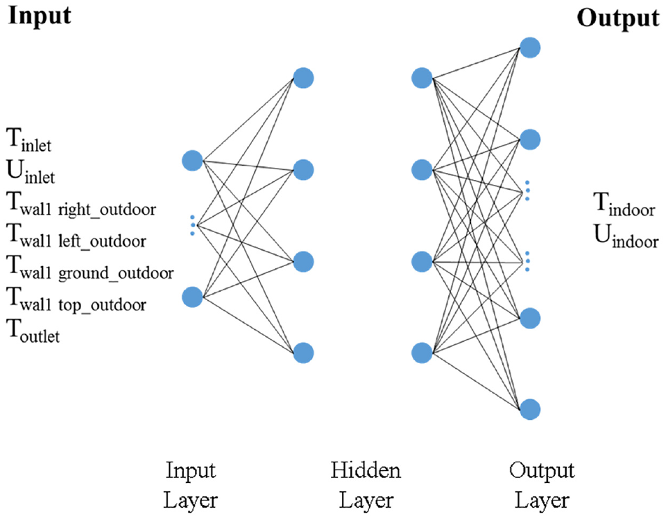
In the initial phase, conducting CFD simulations under various operational scenarios and subsequently comparing the obtained results. Furthermore, the data generated from the CFD simulations played a crucial role in training the DNN model. Figure 1 illustrates the interconnected CFD-based DNN model, a two-step process. In the first step, the CFD simulation process involves configuring an initial model with geometric construction. Subsequently, data extraction is performed to generate input data for the DNN model during the post-processing phase. The second stage features the DNN model, primarily composed of pre-processed CFD simulation data within both training and testing datasets. Following the training phase, predictions were executed using the DNN model and then validated by comparing them to the results obtained from the CFD simulations. Notably, the DNN model incorporates an input layer encompassing key parameters, namely, inlet velocity, inlet/outlet temperature, and wall temperature, and utilizes the Adam optimizer as part of its loss function. Subsequent subsections describe in more detail the steps taken to fulfil the study aims previously mentioned.

Figure 1.

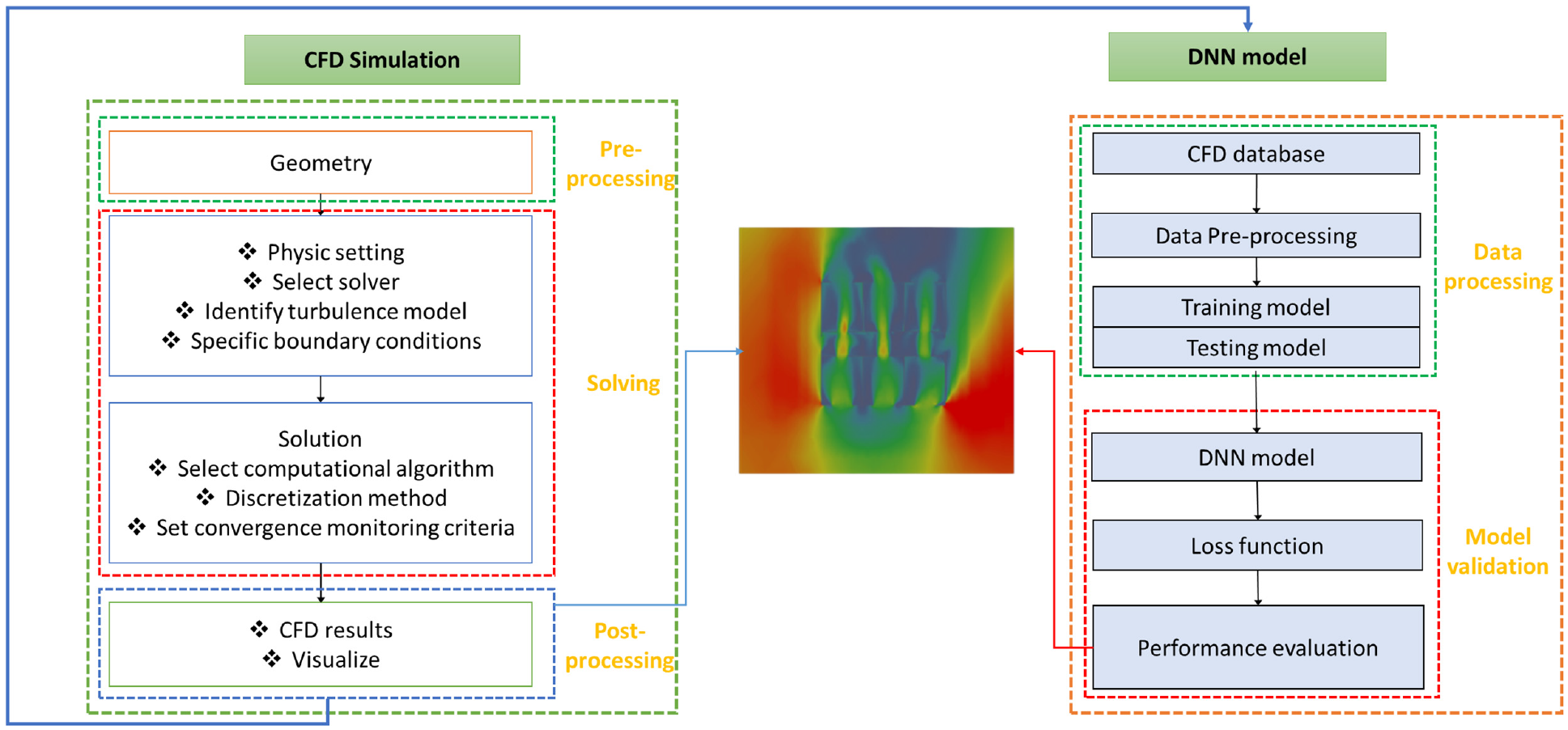
Schematic diagram of the coupling of a CFD-based DNN model.

Generic space

The generic space used in this study consists of a residential building with the following dimensions: L × W × H = 9 m × 9 m × 17.7 m. This building comprises six storeys, and each floor includes a corridor and six rooms, each with dimensions L × W × H = 3 m × 3.6 m × 2.9 m. Each room has one window, measuring W × H = 1.5 m × 1.5 m. Additionally, the corridor windows have dimensions W × H = 0.9 m × 1.5 m, with two windows on each floor. As shown in Figure 2, the residential building was generated on Rhinoceros 7 software (Robert McNeel & Associates, 2008).

Figure 2.

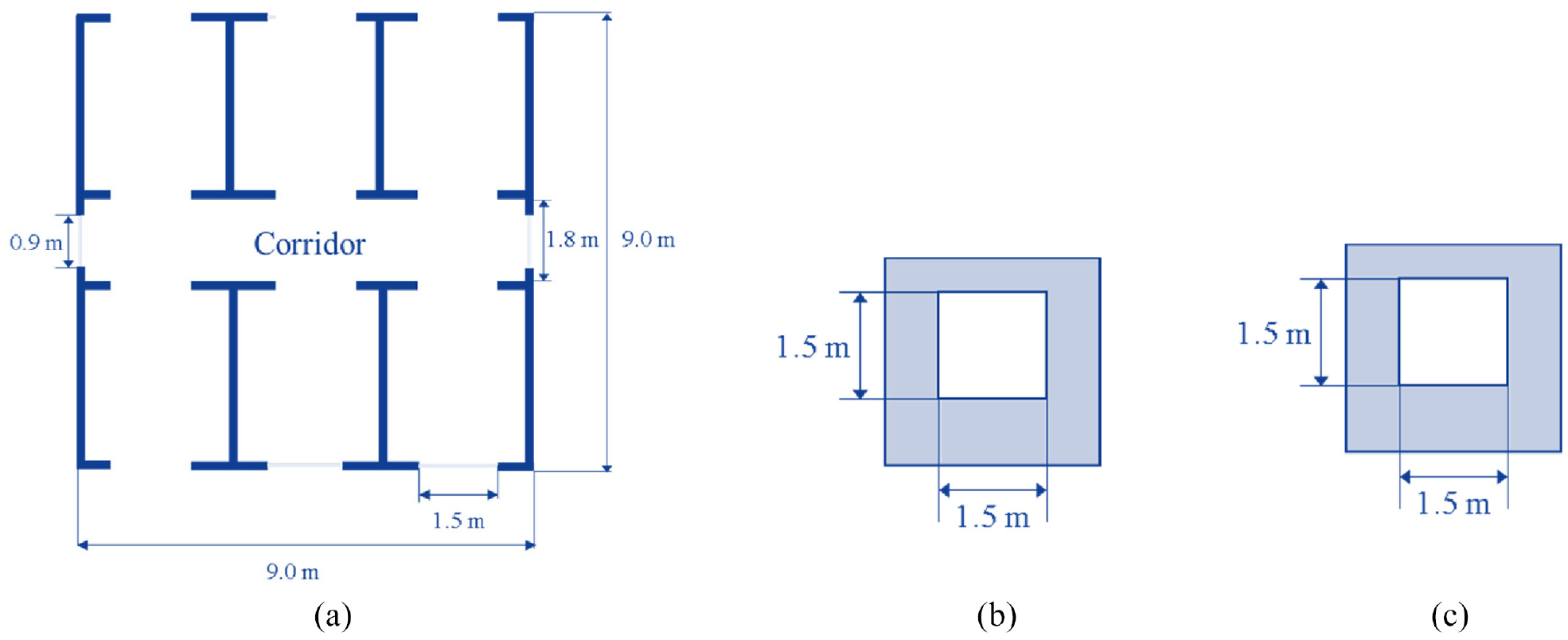
Geometrical dimensions of the residential building: (a) cross-section of the residential building, (b) window at each room, and (c) window in the corridor.

CFD modeling

Governing equations and turbulence models

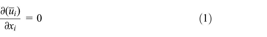
The airflow within the computational domain is modeled for the incompressible fluid phase, and the governing equations for mass and momentum are expressed as follows (1) and (2).

\frac{\partial ({\bar{u}}_{i})}{\partial x_{i}} = 0

(1)

\frac{\partial ({\bar{u}}_{i})}{\partial t} + u_{j} \frac{\partial u_{i}}{\partial x_{j}} = - \frac{1}{ρ} \frac{\partial p}{\partial x_{i}} + \frac{\partial}{\partial x_{j}} (2 ν S_{ij} - \bar{u_{i}' u_{j}'})

(2)

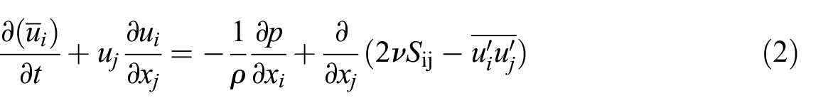
In the context of the equation discussed, the variable ν represents the kinematic viscosity, S_ij corresponds to the strain–rate tensor, p donates the mean pressure, ρ represents the air density, $u'$ represents the fluctuating velocity component and ${\bar{u}}_{i}$ denotes the ensemble-average velocity.

- \bar{u_{i}' u_{j}'} = 2 v_{t} S_{ij} - \frac{2}{3} k δ_{ij}

(3)

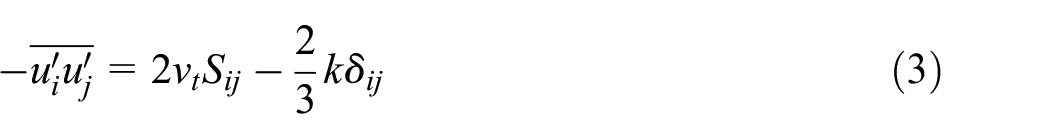
In the considered framework, the variable k represents the turbulent quantity, δ_ij represents the Kronecker delta, and the turbulent or eddy velocity (ν_t) is determined using the RANS model for eddy viscosity modeling.

The power law has been applied to the inlet by defining the atmosphere boundary condition.

U (z) = \frac{u^{*}}{k} \ln (\frac{z}{z_{0}})

(4)

k (z) = \frac{3}{2} (U (z) . T_{i})

(5)

ε (z) = C_{μ}^{3 / 4} \frac{k^{3 / 2}}{l_{t}}

(6)

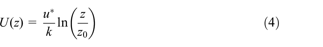
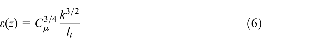
In the given equations, U represents the mean wind velocity, y denotes the height, and u* refers to the atmospheric boundary layer (ABL) friction velocity (u* = 2.89 m/s). The von Karman constant, denoted as k, is taken as 0.415. Equations (5) and (6) represent the turbulent kinetic energy and dissipation rate, respectively. The model constant $C_{μ}$ is assigned a value of 0.09. The initial boundary conditions were measured for the simulations and presented in Table 2. To cover a range of typical scenarios, the ratios between intake velocity and temperature values were adjusted for each case, including 29 cases for analysis and evaluation (see Table 3). The Reynolds-averaged Navier-Stokes (RANS) simulations for indoor airflow distribution in a multi-story residential building designed for natural ventilation. The inlet velocity values were set to a minimum of 2 m/s across all scenarios, ensuring that the flow field exhibited Reynolds number independence. This approach focuses on the relative airflow velocities at the inlets, reducing the number of cases required to construct the database while maintaining the integrity of results.

Table 2.

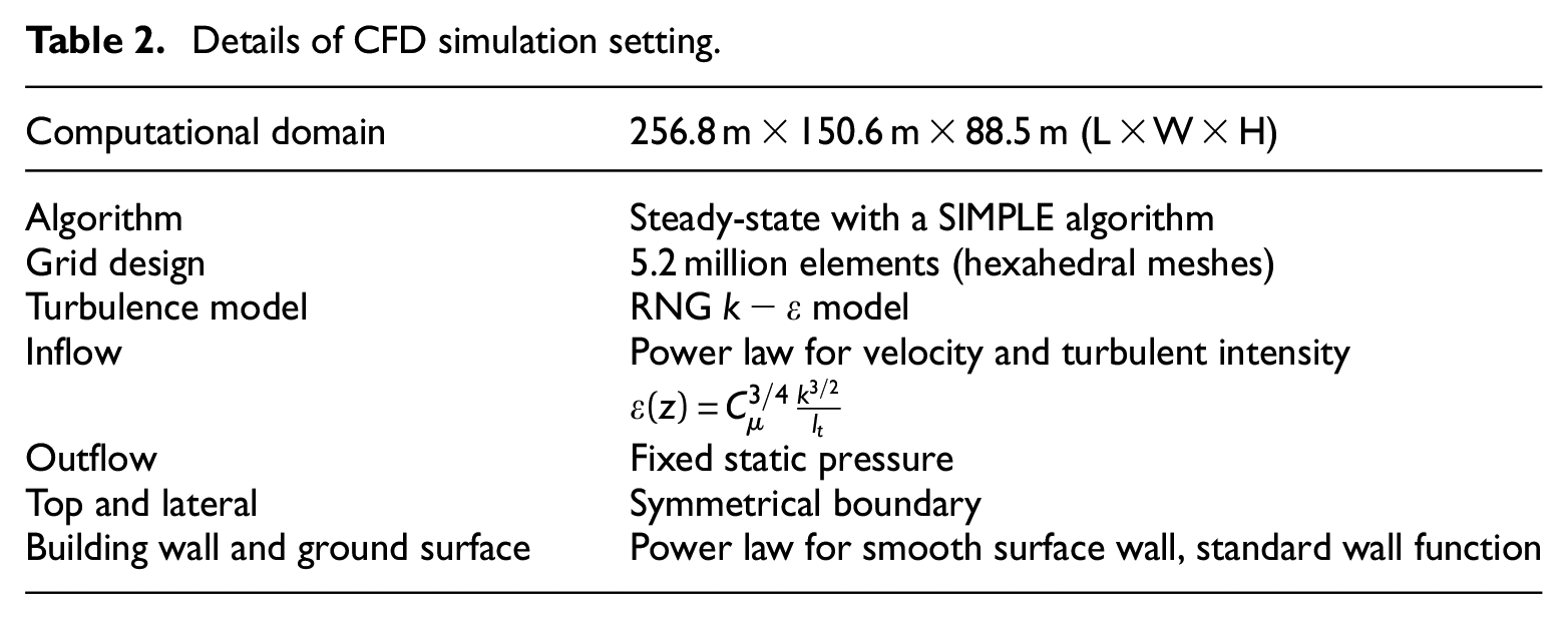
Details of CFD simulation setting.

Computational domain	256.8 m × 150.6 m × 88.5 m (L × W × H)
Algorithm	Steady-state with a SIMPLE algorithm
Grid design	5.2 million elements (hexahedral meshes)
Turbulence model	RNG k − ε model
Inflow	Power law for velocity and turbulent intensity $ε (z) = C_{μ}^{3 / 4} \frac{k^{3 / 2}}{l_{t}}$
Outflow	Fixed static pressure
Top and lateral	Symmetrical boundary
Building wall and ground surface	Power law for smooth surface wall, standard wall function

Table 3.

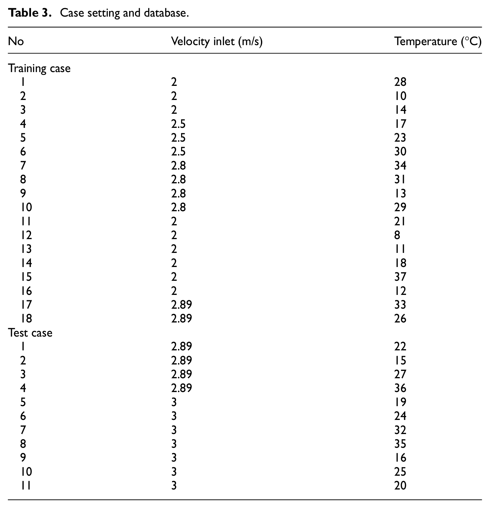
Case setting and database.

No	Velocity inlet (m/s)	Temperature (°C)
Training case
1	2	28
2	2	10
3	2	14
4	2.5	17
5	2.5	23
6	2.5	30
7	2.8	34
8	2.8	31
9	2.8	13
10	2.8	29
11	2	21
12	2	8
13	2	11
14	2	18
15	2	37
16	2	12
17	2.89	33
18	2.89	26
Test case
1	2.89	22
2	2.89	15
3	2.89	27
4	2.89	36
5	3	19
6	3	24
7	3	32
8	3	35
9	3	16
10	3	25
11	3	20

When applying CFD for natural ventilation calculations, selecting an appropriate turbulence model significantly influences simulation accuracy and necessitates careful consideration. CFD commonly employs the RANS equations or Large Eddy Simulation (LES; Blocken, 2018). The RANS equations are often coupled with two-equation turbulence closure models, such as the standard k − ε model (SKT), the realizable k − ε model (RLZ), and the renormalized group k − ε model (RNG; Blocken, 2014, 2018; Chen, 2009). RANS simulations have investigated factors affecting natural ventilation, including building geometry, ventilation apertures, ambient wind speed, wind direction, and simulation parameters like domain size, grid resolution, and turbulence closure model selection (Ai & Mak, 2014b; Cheng-hu et al., 2016; Derakhshan & Shaker, 2017; van Hooff et al., 2017). RANS simulations are computationally efficient, require less time, and offer greater adaptability (Blocken, 2018). However, they do have certain limitations that may compromise accuracy. Notably, RANS cannot resolve fluctuating flow variables, necessitating the exclusion of turbulent components from the simulation (Ai & Mak, 2014a, 2014b; Caciolo et al., 2012; van Hooff et al., 2017). Additionally, two-equation turbulence closure models often struggle to capture vortex shedding accurately, leading to over-prediction of turbulent kinetic energy around the stagnation point and flow recirculation near the simulated building (Blocken, 2018). LES can be employed to address these limitations, which explicitly models turbulence and provides more realistic flow data, including flow intermittencies and separations around the building. LES can resolve governing equations for eddies larger than the subgrid-scale (Sørensen & Nielsen, 2003). However, LES requires additional computation, making it less widely used than RANS. Its applications are typically limited to investigating how building geometry, orifice locations, and computational settings influence the natural ventilation rate (Ai & Mak, 2014a, 2014b; Caciolo et al., 2012; Evola & Popov, 2006; Jiang & Chen, 2002; van Hooff et al., 2017; Wang & Chen, 2012).

Grid design

The residential building model is located inside a computational domain with distances from their inlet, outlet, and the boundary of lateral (left and right) to their nearest surfaces of 4H, 10H, and 4H, respectively, and the height of the computational domain is 5H, shown in Figure 3.

Figure 3.

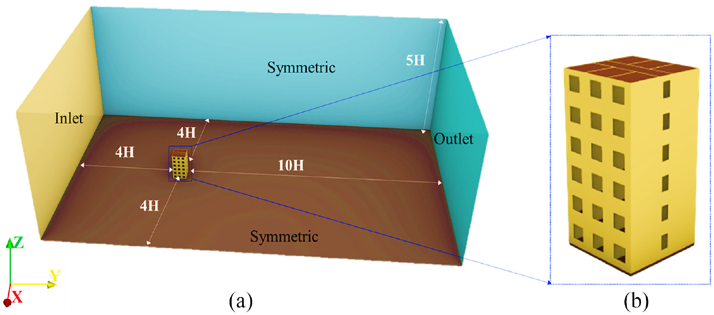
The residential building 3D model: (a) computational domain and (b) residential building.

A 3D grid is very significant to get reliable and accurate CFD results. The structure grids were created to represent the shape of the computational domain by using OpenFOAM (Greenshields, 2021). The meshing generation consists of the following steps. First, the 3D model was constructed and exported in STL (stereolithography) file format on Rhinoceros 7 software (Robert McNeel & Associates, 2008). The next step was to build a computational domain surrounding the residential building and create an initial background mesh using the OpenFOAM blockMesh utility. The third step was to split cells at building walls and in regions of interest using the SnappyHexMesh utility of the OpenFOAM. The final step was to check the mesh quality and delete bad-quality cells no longer refined. The computational grid was fully structured, being more refined near the area of interest, the immediate surroundings of the building model. The computational grid is a structure grid, and the site of the target building was refined. Minimum and maximum layer thickness were 0.01 and 0.3, respectively, with an expansion ratio of 1.1, guaranteeing a smooth transition from fine mesh near the wall surfaces and avoiding significant aspect ratios that can compromise convergence., as shown in Figure 4.

Figure 4.

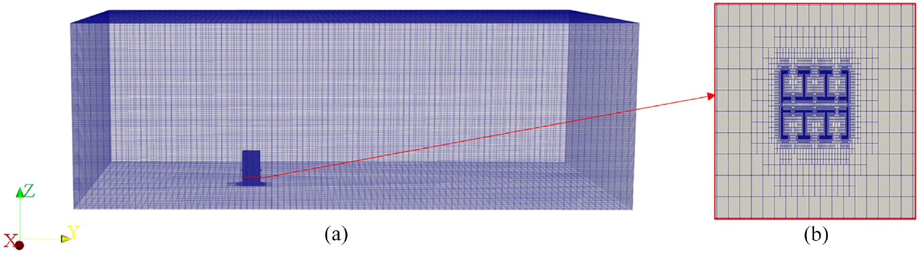
Structure hexahedral finite-volume mesh of the residential building: (a) and (b) horizontal plane at z = 1.5 m.

CFD simulation validation

The velocity components predicted by the RANS model were compared to experimental findings to illustrate the accuracy of the numerical simulations. The flow condition and building size were based on Mu et al. (2016) wind tunnel experiment, which employed a wind tunnel to determine the velocity field within a multistory residential building. The 1:30 scale replicates the full-size model’s width, length, and height. The simulation results and normalized velocity U/Uref distribution data on a cross-measurement line are shown in Figure 5. The blue rhombus symbols indicate Mu et al. (2016). The solid green line represents the simulation results.

Figure 5.

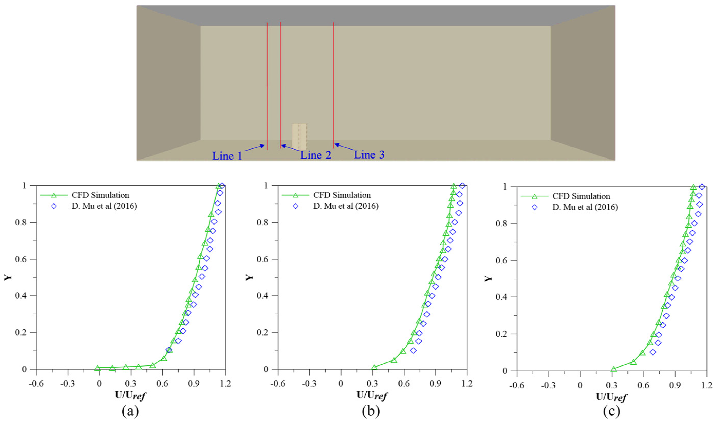
Comparison between CFD predictions (solid line) and experimental measurements (dotted line) of velocity profiles along different sections of the model (lines 1–3).

The velocity profiles and streamwise positions were also compared in this investigation, as shown in Figure 5. The velocity profiles predicted by CFD on the upstream side of the building (lines 1 and 2) accorded exceptionally well with the experimental results. However, CFD could not obtain accurate simulation results with experimental measures downstream from the building model (line 3). According to Jiang and Chen (2001), only LES can produce an accurate forecast. At the same time, Alloca (2001) found that CFD using the RANS turbulence model could not predict the velocity distribution effectively for the wake zone behind the building model. The mean absolute divergence between simulation and experimental data for the whole section is 0.090. The comparison demonstrates that the velocity findings coincide with the data from the reference research, indicating that CFD can recreate the velocity trend.

DNN model and optimization

The DNN model, an evolution of ANN, possesses a more intricate architecture that enables the creation of complex mapping functions from input to output data (Liu et al., 2017). A feedforward DNN consists of an input layer, multiple hidden layers, and an output layer. Each layer houses one or more neurons, and these neurons establish connections with neurons in both the preceding and subsequent layers. In the forward pass process, a neuron takes inputs from the previous layer, applies a nonlinear activation function to these inputs, and then transfers the results to neurons in the following layer. Equation (7) is commonly employed to compute a neuron’s output. Using nonlinear activation functions allows DNNs to handle highly nonlinear relationships between input and output variables. During the training phase, the weights and biases of each neuron are iteratively adjusted until optimal values are achieved. Error propagation (loss) plays a crucial role in this process, wherein the discrepancy between expected and actual values is propagated to the layers above. Various techniques, such as gradient descent approaches, optimize the weights and biases. The application of DNN designs has garnered significant attention and has led to groundbreaking achievements, particularly in computer vision tasks (Jogin et al., 2018). Notably, the scope of DNN’s application extends beyond image-type data and encompasses time-series data as well (Li et al., 2017):

\hat{y} = f (\sum_{i = 1}^{n} w_{i} x_{i} + b)

(7)

Where x_i represents i input of the neuron (the output of a neuron of a previous layer), w_i is the weight between the two neurons, b is the neuron’s bias, and f represents the activation function.

R², MSE, and MAE error measures to assess and compare the performance of the developed algorithms. They may be summed up as follows:

R^{2} = 1 - [\frac{\sum_{i = 1}^{m} {(y_{i} - {\hat{y}}_{i})}^{2}}{\sum_{i = 1}^{m} {(y_{i} - \bar{y})}^{2}}]

(8)

RMSE = \sqrt{\frac{\sum_{i = 1}^{m} {(y_{i} - {\hat{y}}_{i})}^{2}}{m}}

(9)

M A E = \frac{1}{m} \sum_{i = 1}^{m} | y_{i} - {\hat{y}}_{i} |

(10)

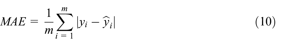
Three fitness metrics, namely R² (coefficient of determination), RMSE (root mean square error), and MAE (mean absolute error), were utilized to assess the model predictions against the actual output. The model predictions are represented by $\hat{y}$ , and the actual output is denoted by y, while $\bar{y}$ signifies the output mean, and m is the number of samples. R² involves normalizing the mean error, making it widely used in the literature for regression-type prediction tasks, including indoor temperature prediction. The output of R² ranges between 0 and 1, with a value of 1 corresponding to a perfect prediction. On the other hand, RMSE considers the squared error term, making it sensitive to extreme values and facilitating the evaluation of outlier predictions and their effects. Meanwhile, MAE provides a direct comparison of performance without emphasizing severe errors. Additionally, since MAE considers differences between actual and predicted values directly, it does not downplay values that may lie between 0 and 1, as observed in the RMSE calculation. By employing these three fitness metrics, a comprehensive and in-depth analysis of the results was conducted, facilitating a more thorough interpretation of the predictive model’s performance.

This study employs a deep learning model with hidden layers and a feedforward architecture (Figure 6). The input layer receives the input vector and external environmental circumstances, while the output layer generates the temperature and velocity data. Neurons in the layer above process signal from the layer below and transmit them onward. The resulting output vector is converted into temperature and velocity tensors, representing the building’s three-dimensional temperature and velocity distributions. Experimental results are the basis for most boundary conditions and are consistently maintained across various scenarios. Hyperparameters in DNNs encompass critical parameters such as the number of hidden layers, neurons within each hidden layer, activation functions, learning rates, and gradient descent algorithms. In this study, we employed Grid Search, an optimization technique, to meticulously fine-tune these hyperparameters (Courville, 2016). Our approach involved training DNNs across various combinations of this finite set of hyperparameters, subsequently selecting the optimal configuration based on validation loss. We thoughtfully defined a compact search space for hyperparameters, balancing the pursuit of accuracy with computational efficiency during the Grid Search algorithm implementation. Detailed hyperparameter settings are provided in Table 4.

Figure 6.

Outline of DNN model.

Table 4.

Hypermeter setting for DNN.

Number of hidden layers	1/3/5
Number of neurons per hidden layer	20/40/80/120/200
Activation function	Tanh
Gradient descent algorithm	Adam
Learning rate	0.001
Batch size	1

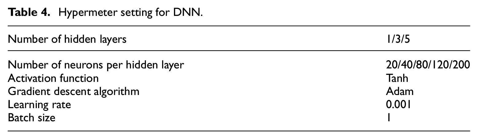
Determining when to stop training is crucial in the training process due to its nonconvex and iterative nature. The training is considered complete when the monitored metric, that is, the validation error, ceases to decrease consecutively for 5000 epochs. At this stage, the training is deemed to have reached convergence. Following termination, the parameters at the early-stopping point are retrieved. Subsequently, the DNN model undergoes testing using the testing data for performance evaluation. Table 4 presents the statistical performance of the velocity and temperature forecasting model.

Results and discussion

DNN model performance

The CFD model for cross ventilation was developed based on the arrangement of a six-storey building driven by buoyancy effects, with adjustments made to match the experimental conditions (refer to Figure 2). To maintain the flow around the building; the wind profile intake was positioned at five-building heights (5H) in front of and on each side of the building, ensuring that the outer domain did not interfere with the airflow patterns. An area four times the block’s height was considered to accommodate the recirculation zone around the three-dimensional block. The outlet was strategically positioned at ten building heights (10H) downwind of the building to prevent flow disruption. Additionally, an upper barrier unaffected the airflow, positioned at four-building heights (4H) above the building.

The primary objective of this study is to predict the airflow distribution within residential buildings, assess its influence on comfort conditions, and mitigate indoor air pollution. Upon analyzing the airflow patterns in the rooms of the residential building, it is evident that inadequate airflow exists, particularly in the bedroom, where airflow enters from multiple directions. Properly designed ventilation systems can play a crucial role in reducing indoor air pollutants and enhancing overall indoor air quality. The case shown in Figure 7, demonstrates airflow distribution of CFD simulation and DNN predictions, the air temperature near external and internal wall openings is determined to be 30°C and velocity inlet to be 2.5 m/s.

Figure 7.

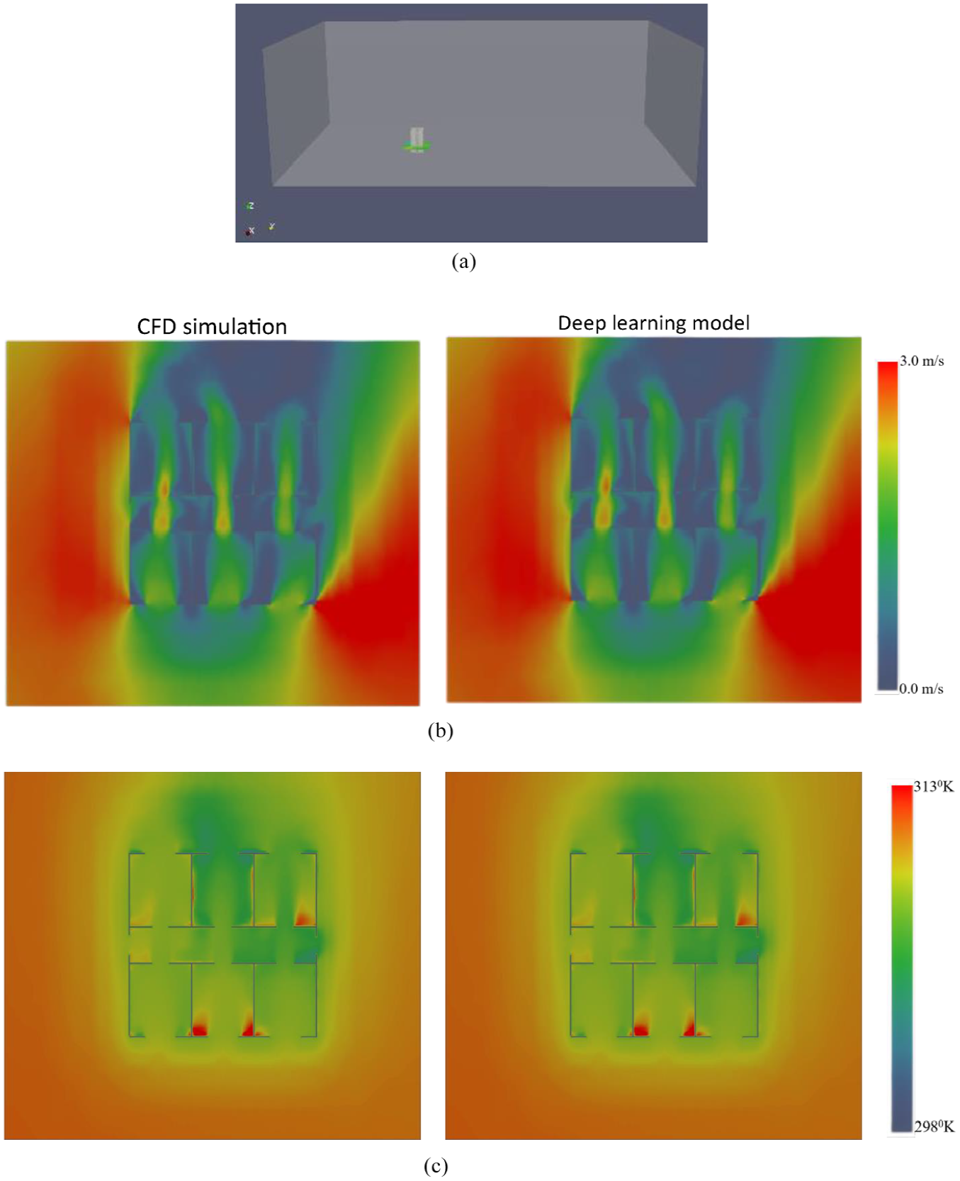
Comparison between CFD simulation (buoyant simple foam) and deep learning prediction, showing both velocity and temperature fields in buildings (floor 3): (a) cross-section location in buildings, (b) velocity distribution, and (c) temperature distribution.

In Figure 7(b), the airflow pattern on a horizontal plane within the building model at an intermediate height (4.5 m above the floor) is depicted when the wind direction is typical to the window and a door is opened. The airflow patterns observed during cross-natural ventilation mode under average wind direction revealed notable convolutions, particularly on the indoor and leeward sides of the structure. The airflow penetrated directly through the windows and doors of the building units, generating multiple vortexes in the corridor and leeward side surrounding the apertures. Additionally, the walls obstructed the airflow, leading to circulations throughout the room. Subsequently, the deep learning model findings (Figure 7(b)) showcased a similar flow pattern trend, with minor differences in the recirculation details deemed acceptable. The wind direction plays a crucial role in modifying the pressure differential between the two openings, thereby influencing the ventilation pace throughout the building. The effect of wind direction on the ventilation rate should be predicted using design tools. A comparison of the ventilation rate calculated by CFD to that obtained through the deep learning model demonstrated that the ventilation rate was maximized when the wind direction was normal to the window opening. The DNN successfully predicted this pattern, and the computed ventilation rate agreed with the CFD simulation result. Hence, the DNN model proved effective in forecasting the impact of wind direction on natural ventilation.

Figure 7(c) illustrates the efficient indoor temperature distribution within the room. The static temperature within the indoor spaces of the building exhibits fluctuations ranging from 298 to 313°K. Notably, the air temperature near external and internal wall openings is determined to be 30°C. The temperature increase within the large central part of the cavities is attributed to natural convection. Furthermore, the temperature distribution is influenced by strongly directed advection. The wind direction was identified as a critical factor, as the volume-weighted average accuracy findings indicated minimal temperature variation between the floors. Moreover, the accuracy of the measurement points was also considered insignificant.

Figure 7(c) compares the estimated temperature profiles obtained from the CFD simulation and the DNN model at a height of 4.5 m to analyze the temperature distribution within the buildings. Both the CFD simulation and the DNN model successfully predicted the presence of heat stratification. The temperature distribution generated by the DNN model exhibited a relatively close agreement with the findings from the CFD simulation. Additionally, the DNN model accurately predicted that the most significant thermal stratification occurs near the walls, consistent with the results of the CFD simulation. Furthermore, Figure 7 presents the temperature fields obtained from the CFD simulation and the DNN model, the temperature field predicted by the DNN model and the percentage error between them. Notably, the figure demonstrates that the error varies within a narrow range of 0.3%, indicating the DNN model’s capability to effectively capture the complex nature of the indoor temperature distribution. Consequently, the model holds promise for anticipating various scenarios in the indoor built environment.

Figure 8 illustrates the agreement between the CFD findings and DNN predictions (indoor velocity and temperature) on the training dataset. Most airflow velocity and temperature values from the CFD simulations align with those from the deep learning predictions. The DNN model can reprogram the airflow field for the examples in the training dataset effectively. However, on the test dataset, the scatter distributions are less compact than the DNN model training dataset, consistent with the observations in Figure 7. This indicates relatively minor discrepancies in the test case predictions compared to the training case predictions. Despite this, it suggests that the DNN outperforms the test dataset compared to the training dataset. Additionally, it is noteworthy that the consistency of the DNN’s velocity and temperature data is comparable to that of the CFD results.

Figure 8.

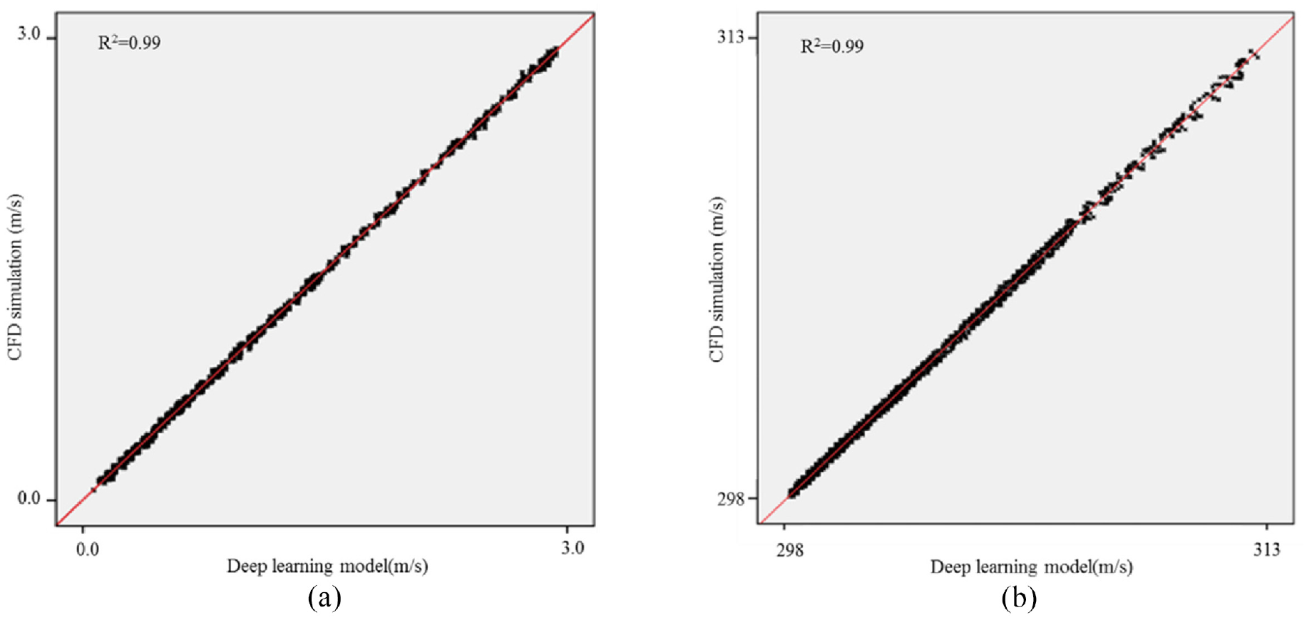
Correlations between CFD simulation results and deep learning predictions: (a) indoor air velocity and (b) indoor air temperature.

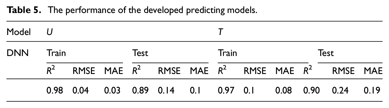
Figure 8 demonstrates that the relative error for the forecasted velocity and temperature is less than 0.5%, indicating the DNN model’s capability to capture the variance in velocity and temperature accurately. The relative error is approximately 5%, with a few outliers exhibiting near-zero void fractions. Based on the previously mentioned morphological parameters, we developed the DNN prediction model. Various architectures with neuron counts ranging from 20 to 200 were evaluated regarding R², RMSE, and MAE, using train-test ratios of 70% (Table 5). Figure 8 also indicates that the DNN model can successfully predict subcooled boiling regimes, closely aligning with the CFD values. The results in Table 5 display the model’s exceptional fit with the validation data, as evidenced by the minimal RMSE value.

Table 5.

The performance of the developed predicting models.

Model	U						T
DNN	Train			Test			Train			Test
	R ²	RMSE	MAE	R ²	RMSE	MAE	R ²	RMSE	MAE	R ²	RMSE	MAE
	0.98	0.04	0.03	0.89	0.14	0.1	0.97	0.1	0.08	0.90	0.24	0.19

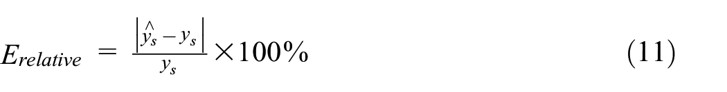
To quantify the difference between CFD simulations and DNN predictions, equation (11). defines an evaluation criterion, namely the relative error.

E_{r e l a t i v e} = \frac{| \overset{\land}{y_{s}} - y_{s} |}{y_{s}} \times 100 %

(11)

where ${\hat{y}}_{s}$ is the DNN prediction value at one place, y_s is the CFD real value at the same point, and s is the location.

The DNN models are known for their computational efficiency, allowing for the exclusion of computation time from the model evaluation. Figure 9 shows the DNN’s accuracy in training and validation procedures based on the Mean Absolute Error (MAE). The DNN model demonstrates precise predictions of indoor airflow on the test dataset. However, it is essential to note that none of the DNN models exhibited excessive accuracy on the training dataset, suggesting their ability to adapt to new design inputs for accurate ventilation rate predictions. The statistical analysis of the velocity and temperature forecasting model can be found in Table 5.

Figure 9.

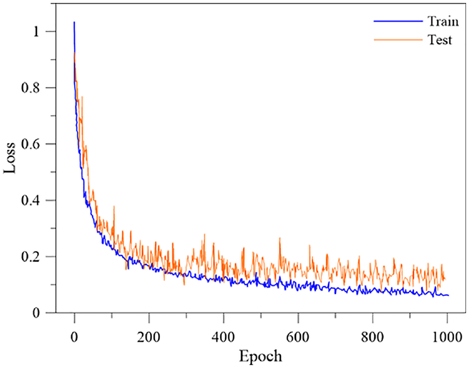
The MAE-based DNN model training procedure.

Figure 10 illustrates the quantified relative errors derived from DNN predictions on the test dataset. These relative errors exhibit varying degrees of increase, with the DNN model displaying mean relative error values exceeding 6%, surpassing those observed on the training dataset. Furthermore, notable variations in relative error for the DNNs are evident. While achieving consistent performance between test and training datasets would be ideal, it is essential to acknowledge that performance degradation on test datasets is an inherent challenge. Essentially, the DNN has already acquired a deep understanding of the airflow patterns within the training cases. Therefore, when predicting test cases, it leverages the learned mappings from the training phase to anticipate airflow patterns in unfamiliar scenarios, resulting in larger prediction errors for the test cases compared to the training cases.

Figure 10.

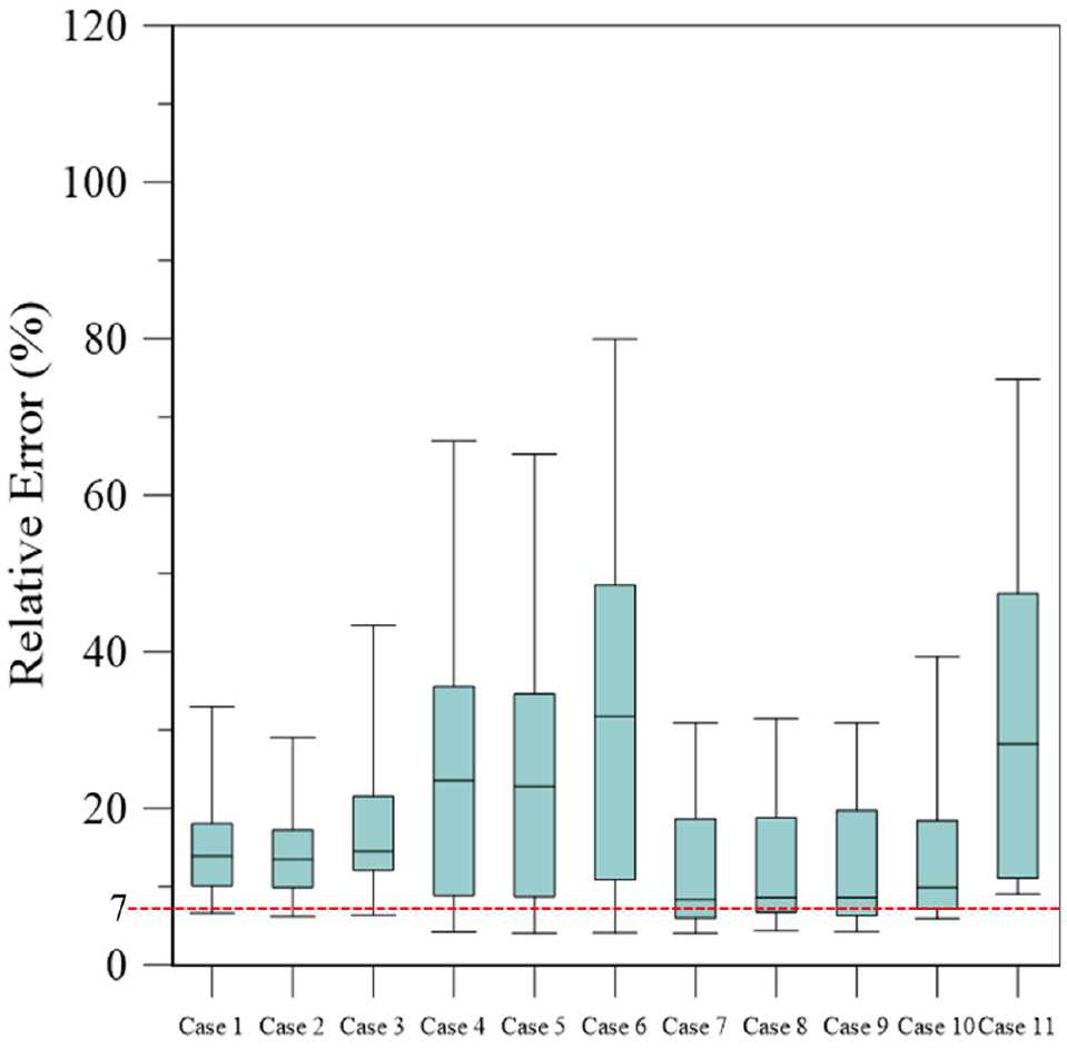
Relative error of DNN model.

Computational time

Computational time plays a crucial role in assessing the efficiency of the prediction models. This study compared the CPU-CPU time for a fair evaluation since GPU reference time measurements were unavailable. We considered the average solution time to account for variations in CFD solution durations due to pressure-velocity coupling features. Increasing the batch size minimally affected the CPU run speed. Still, we also evaluated GPU evaluation durations, as machine learning models can be executed on GPUs, leading to varying forecast timeframes based on the batch size.

Apart from prediction accuracy, calculation time is an essential factor to consider. The computation time in our study refers to the total time spent predicting temperature and velocity distributions for the 29 testing instances. For CFD simulations, the calculation time is simply the time it takes to run the simulations. In contrast, for the DNN model, the calculation time includes the time spent creating training data and conducting DNN training. The DNN model takes less than a second to provide the expected values and is negligible during computation. CFD simulations were performed for various scenario cases on the hardware platform (Linux with an Intel Core i9-10900X CPU 3.70 GHz). When utilizing multiple cores and processors in parallel, it took approximately 20 h per case, nine times faster than a single CPU.

Conversely, DNN installation and training required around 5 h to train the model. Figure 11 compares the computation time for predicting the 29 testing scenarios between the DNN model and CFD. While CFD took approximately 8 h for the 29 testing instances, the DNN model resulted in an 80% decrease in overall time compared to CFD simulations. The term “quick” reflects this speed improvement in two ways: first, the time consumption for CFD simulations significantly decreased due to fewer examples used for training data, and second, the well-trained DNN accurately predicts unknown scenarios instantaneously.

Figure 11.

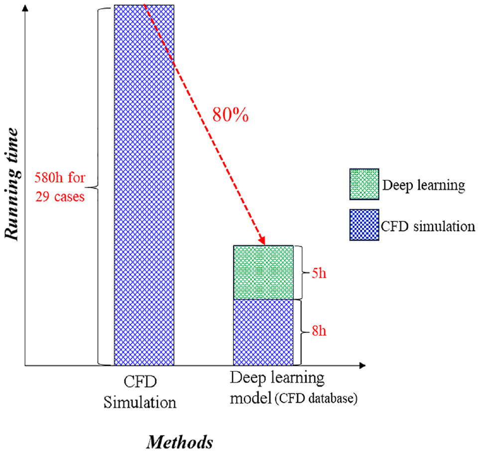
Comparison of computation time for predicting cases between Deep learning model and CFD simulation.

Future work and conclusions

This article established a framework for systematizing studies of a building’s wind-driven natural ventilation potential through CFD simulation and a deep learning model. The study proposed using numerical simulation and deep learning models for either building design or assessment by integrating available programs and providing bespoke features. As a baseline, a full-scale test home was employed. As a reference, its geometry and the climatic conditions of its location were established, and air velocity measurements within the experimental home served as validation data.

This study aimed to forecast indoor airflow and temperature dispersion using a DNN. DNN model architectures were built with this in mind. DNN depicts a DNN that simultaneously predicts velocity and temperature values for the entire domain. DNN prediction performance was evaluated using both the training and test datasets. For evaluating DNN prediction performance, the relative error between CFD simulation results and DNN predictions was utilized as an assessment criterion. In the training dataset, the relative errors of DNN predictions varied somewhat. The study presents a data-driven approach that combines CFD simulations with machine learning techniques to predict indoor airflow in multi-storey residential buildings. The quantitative findings demonstrate the DNN’s ability to accurately forecast indoor airflow patterns and temperature distributions. Notably, the DNN model outperforms traditional CFD simulations by achieving an 80% reduction in computational time for predicting testing scenarios. This research highlights the feasibility and effectiveness of our data-driven approach, offering swift and precise indoor airflow predictions in naturally ventilated residential buildings. These predictive models have the potential to significantly enhance indoor air quality, thermal comfort, and energy efficiency, contributing to sustainable building design and operation.

Meanwhile, DNN maintained its accuracy. Finally, for each example, the prediction speed of a well-trained DNN is much quicker than CFD simulation. DNN has been promising for speedy and accurate indoor environment prediction in practical applications. Although low Reynolds number flows are generally suitable for many domains, such as architectural design, higher Reynolds number flows should be investigated to expand the technique to additional areas of design optimization. It would also be essential to examine whether the findings of our approximation models may be used as a warm-up setting for high-accuracy CFD simulations. The number of iterations necessary to connect to steady-state might be significantly decreased because the forecasts are near approximations of the final, wholly converged outcomes. As a result, classic CFD approaches with excellent accuracy might be made to assemble significantly faster.

In terms of future work, the stage has been set by this study for several promising research directions. Firstly, the need for practical application is highlighted, involving field studies to validate and fine-tune our data-driven predictive models in real-world multi-storey residential buildings, considering various environmental conditions and architectural configurations. Secondly, the applicability of our approach to a broader spectrum of flow conditions, including higher Reynolds numbers, is to be explored in further investigations. Additionally, the potential for integrating our data-driven models with building management systems (BMS) is recognized for enabling real-time indoor airflow predictions and energy-efficient building operation. Efficiency gains are another area of focus, with ongoing research aimed at optimizing computational speed while maintaining accuracy. Furthermore, the expansion of the reach of our approach beyond residential settings to domains like urban planning, industrial facilities, and healthcare environments is warranted. Lastly, addressing limitations, such as the need for extensive training data and model generalization, remains integral to the advancement of the practicality and effectiveness of our predictive models. In summary, the study presents a roadmap for future research that encompasses practical application, model robustness, BMS integration, computational efficiency, multi-domain versatility, and continuous efforts to overcome limitations in indoor airflow prediction for sustainable building design and operation.

Footnotes

Appendix A

Acknowledgements

The author would like to express our sincere appreciation to The Human Behaviour and Energy Laboratory (HuBEL) at the Kyung Hee University, the Republic of Korea, supported facilitates research.

Author contributions

The author contributed equally to the preparation of this manuscript.

Declaration of conflicting interests

The author(s) declared no potential conflicts of interest with respect to the research, authorship, and/or publication of this article.

Funding

The author(s) disclosed receipt of the following financial support for the research, authorship, and/or publication of this article: This research has been supported with a Presidential Scholarship from Kyung Hee University, Republic of Korea.

ORCID iD

Tran Van Quang

References

Mak

(2014a) Determination of single-sided ventilation rates in multistory buildings: Evaluation of methods. Energy and Buildings 69: 292–300.

Mak

(2014b) Modeling of coupled urban wind flow and indoor air flow on a high-density near-wall mesh: Sensitivity analyses and case study for single-sided ventilation. Environmental Modelling and Software 60: 57–68.

Allocca

(2001) Single-sided natural ventilation: design analysis and general guidelines [Doctoral dissertation]. Massachusetts Institute of Technology.

Al-qahtani

(1993) Subjective assessment of indoor air quality in office buildings [Doctoral dissertation]. King Fahd University of Petroleum and Minerals.

Berger

Aftosmis

Marshall

, et al. (2005) Performance of a new CFD flow solver using a hybrid programming paradigm. Journal of Parallel and Distributed Computing 65(4): 414–423.

Blocken

(2014) 50 years of computational wind engineering: Past, present and future. Journal of Wind Engineering and Industrial Aerodynamics 129: 69–102.

Blocken

(2015) Computational Fluid Dynamics for urban physics: Importance, scales, possibilities, limitations and ten tips and tricks towards accurate and reliable simulations. Building and Environment 91: 219–245.

Blocken

(2018) LES over RANS in building simulation for outdoor and indoor applications: A foregone conclusion? Building Simulation 11(5): 821–870.

Caciolo

Stabat

Marchio

(2012) Numerical simulation of single-sided ventilation using RANS and LES and comparison with full-scale experiments. Building and Environment 50: 202–213.

10.

Chen

(2009) Ventilation performance prediction for buildings: A method overview and recent applications. Building and Environment 44(4): 848–858.

11.

Chen

Tong

Zheng

, et al. (2020) Transfer learning with deep neural networks for model predictive control of HVAC and natural ventilation in smart buildings. Journal of Cleaner Production 254: 119866.

12.

Chen

Jiang

Tong

, et al. (2021) Residual stress distribution design for gear surfaces based on genetic algorithm optimization. Materials 14(2): 366.

13.

Chenari

Dias Carrilho

Gameiro Da Silva

(2016) Towards sustainable, energy-efficient and healthy ventilation strategies in buildings: A review. Renewable and Sustainable Energy Reviews 59: 1426–1447.

14.

Cheng

JCP

Kwok

HHL

ATY

, et al. (2022) BIM-supported sensor placement optimization based on genetic algorithm for multi-zone thermal comfort and IAQ monitoring. Building and Environment 216: 108997.

15.

Cheng-hu

Kurabuchi

Ohba

(2016) Numerical study of cross-ventilation using two-equation RANS turbulence models. International Journal of Ventilation 4(2): 123–131.

16.

Common

(2003) Uncertainty and the environment: implications for decision-making and environmental policy. Richard A. Young. Edward Elgar, Cheltenham, UK; Northampton, MA, 2001. ISBN 1 84064 626 8 (hardcover, 59.95 pounds sterling, $85.00). Journal of Economic Psychology 24(3): 422–424.

17.

Cook

(2008) Rhinoceros NURBS modeling for window, training manual level 1 version 4.0. Robert McNeel and Associates.

18.

Cook

Hunt

(2003) CFD modelling of natural ventilation: Combined wind and buoyancy forces. International Journal of Ventilation 1(3): 169–179.

19.

Cook

Lomas

(1998) Buoyancy-driven displacement ventilation flows: Evaluation of two eddy viscosity turbulence models for prediction. Building Services Engineering Research and Technology 19(1): 15–21.

20.

Costa

Keane

Torrens

, et al. (2013) Building operation and energy performance: Monitoring, analysis and optimisation toolkit. Applied Energy 101: 310–316.

21.

Courville

Goodfellow

Bengio

(2016) Deep learning. Nature 29(7553): 1–73.

22.

Deng

Tan

(2019) Numerical analysis of local thermal comfort in a plan office under natural ventilation. Indoor and Built Environment 29(7): 972–986.

23.

Derakhshan

Shaker

(2017) Numerical study of the cross-ventilation of an isolated building with different opening aspect ratios and locations for various wind directions. International Journal of Ventilation 16(1): 42–60.

24.

Elshafei

Negm

Bady

, et al. (2017) Numerical and experimental investigations of the impacts of window parameters on indoor natural ventilation in a residential building. Energy and Buildings 141: 321–332.

25.

Evola

Popov

(2006) Computational analysis of wind driven natural ventilation in buildings. Energy and Buildings 38(5): 491–501.

26.

Gheziel

Hanini

Mohamedi

(2022) Artificial neural network (ANN) for prediction indoor airborne particle concentration. International Journal of Ventilation 21(1): 74–87.

27.

Gratia

De Herde

(2004) Natural cooling strategies efficiency in an office building with a double-skin façade. Energy and Buildings 36(11): 1139–1152.

28.

OpenFOAM (2021) The OpenFOAM Foundation. Available at: https://openfoam.org/

29.

Guo

Iorio

(2016) Convolutional neural networks for steady flow approximation. In: Proceedings of the 22nd ACM SIGKDD international conference on knowledge discovery and data mining, pp.481–490. New York, NY, USA: Association for Computing Machinery (KDD ’16). Available at: https://doi.org/10.1145/2939672.2939738

30.

Hajdukiewicz

Geron

Keane

(2013) Calibrated CFD simulation to evaluate thermal comfort in a highly-glazed naturally ventilated room. Building and Environment 70: 73–89.

31.

Harbola

Coors

(2019) One dimensional convolutional neural network architectures for wind prediction. Energy Conversion and Management 195: 70–75.

32.

Hintea

Brusey

Gaura

(2015) A study on several machine learning methods for estimating cabin occupant equivalent temperature. ICINCO 2015 - 12th International Conference on Informatics in Control, Automation and Robotics, Proceedings1: 629–634.

33.

Hong

Lee

Kim

(2017) Analysis of energy consumption and indoor temperature distributions in educational facility based on CFD-BES model. Energy Procedia 105: 3705–3710.

34.

Huang

Kuo

(2018) A short-term wind speed forecasting model by using artificial neural networks with stochastic optimization for renewable energy systems. Energies 11(10): 2777.

35.

Huang

Liao

(2022) Development of an indoor environment evaluation model for heating, ventilation and air-conditioning control system of office buildings in subtropical region considering indoor health and thermal comfort. Indoor and Built Environment 31(3): 807–819.

36.

Jamaludin

Hussein

Mohd Ariffin

, et al. (2014) A study on different natural ventilation approaches at a residential college building with the internal courtyard arrangement. Energy and Buildings 72: 340–352.

37.

Jiang

Chen

(2001) Study of natural ventilation in buildings by large eddy simulation. Journal of Wind Engineering and Industrial Aerodynamics 89(13): 1155–1178.

38.

Jiang

Chen

(2002) Effect of fluctuating wind direction on cross natural ventilation in buildings from large eddy simulation. Building and Environment 37(4): 379–386.

39.

Jogin

Madhulika

Divya

, et al. (2018) Feature extraction using convolution neural networks (CNN) and deep learning. In: 2018 3rd IEEE international conference on recent trends in electronics, information & communication technology (RTEICT), 18–19 May 2018, pp.2319–2323. Bangalore, India: Institute of Electrical and Electronics Engineers (IEEE). Available at: https://doi.org/10.1109/RTEICT42901.2018.9012507

40.

Klepeis

Nelson

Ott

, et al. (2001) The National Human Activity Pattern Survey (NHAPS): A resource for assessing exposure to environmental pollutants. Journal of Exposure Analysis and Environmental Epidemiology 11(3): 231–252.

41.

Kolokotroni

Aronis

(1999) Cooling-energy reduction in air-conditioned offices by using night ventilation. Applied Energy 63(4): 241–253.

42.

Zhang

, et al. (2017) Classification of ECG signals based on 1D convolution neural network. In: 2017 IEEE 19th international conference on e-health networking, applications and services (Healthcom), 16 December 2017, p.16. Dalian, China: Institute of Electrical and Electronics Engineers (IEEE). Available at: https://doi.org/10.1109/HealthCom.2017.8210784

43.

Liping

Hien

(2007) The impacts of ventilation strategies and facade on indoor thermal environment for naturally ventilated residential buildings in Singapore. Building and Environment 42(12): 4006–4015.

44.

Liu

Heidarinejad

Gracik

, et al. (2015) The impact of exterior surface convective heat transfer coefficients on the building energy consumption in urban neighborhoods with different plan area densities. Energy and Buildings 86: 449–463.

45.

Liu

Heidarinejad

Pitchurov

, et al. (2018) An extensive comparison of modified zero-equation, standard k-ε, and LES models in predicting urban airflow. Sustainable Cities and Society 40: 28–43.

46.

Liu

Lin

Chou

(2009) Evaluation of buoyancy-driven ventilation in atrium buildings using computational fluid dynamics and reduced-scale air model. Building and Environment 44(9): 1970–1979.

47.

Liu

Wang

Liu

, et al. (2017) A survey of deep neural network architectures and their applications. Neurocomputing 234: 11–26.

48.

Gao

Zhu

(2016) Wind tunnel tests of inter-flat pollutant transmission characteristics in a rectangular multi-storey residential building, part A: Effect of wind direction. Building and Environment 108: 159–170.

49.

Nielsen

(2015) Fifty years of CFD for room air distribution. Building and Environment 91: 78–90.

50.

Park

Chang

(2020) Effects of combined central air conditioning diffusers and window-integrated ventilation system on indoor air quality and thermal comfort in an office. Sustainable Cities and Society 61: 102292.

51.

Wei

(2020) Performance evaluation of climate-adaptive natural ventilation design: A case study of semi-open public cultural building. Indoor and Built Environment 30(10): 1714–1724.

52.

Raja

Nicol

McCartney

, et al. (2001) Thermal comfort: Use of controls in naturally ventilated buildings. Energy and Buildings 33(3): 235–244.

53.

Raji

Tenpierik

Bokel

, et al. (2020) Natural summer ventilation strategies for energy-saving in high-rise buildings: A case study in the Netherlands. International Journal of Ventilation 19(1): 25–48.

54.

Schulze

Eicker

(2013) Controlled natural ventilation for energy efficient buildings. Energy and Buildings 56: 221–232.

55.

Shaikh

Bin

Nor

, et al. (2013) Robust stochastic control model for energy and comfort management of buildings. Australian Journal of Basic and Applied Sciences 7(10): 137–144.

56.

Sørensen

Nielsen

(2003) Quality control of computational fluid dynamics in indoor environments. Indoor Air 13(1): 2–17.

57.

Spalart

Garbaruk

(2021) Correction to: A New “λ2” term for the spalart–allmaras turbulence model, active in axisymmetric flows. Flow, Turbulence and Combustion, 107(2), 245–256.

58.

Tanaka

Matsuoka

Kawakami

, et al. (2019) Optimization calculations and machine learning aimedat reduction of wind forces acting on tall buildingsand mitigation of wind environment. International Journal of High-Rise Buildings 8(4): 291–302.

59.

Tian

Cheng

Lin

(2022) Modelling indoor environment indicators using artificial neural network in the stratified environments. Building and Environment 208: 108581.

60.

Tominaga

Blocken

(2015) Wind tunnel experiments on cross-ventilation flow of a generic building with contaminant dispersion in unsheltered and sheltered conditions. Building and Environment 92: 452–461.

61.

Tominaga

Mochida

Yoshie

, et al. (2008) AIJ guidelines for practical applications of CFD to pedestrian wind environment around buildings. Journal of Wind Engineering and Industrial Aerodynamics 96(10–11): 1749–1761.

62.

Umetani

Bickel

(2018) Learning three-dimensional flow for interactive aerodynamic design. ACM Transactions on Graphics 37(4): 1–10.

63.

van Hooff

Blocken

Tominaga

(2017) On the accuracy of CFD simulations of cross-ventilation flows for a generic isolated building: Comparison of RANS, LES and experiments. Building and Environment 114: 148–165.

64.

Vladimir

(1967) Energy simulation of displacement ventilation in offices. Gastronomía Ecuatoriana y Turismo Local 1(69): 5–24.

65.

Wang

Chen

(2012) A new empirical model for predicting single-sided, wind-driven natural ventilation in buildings. Energy and Buildings 54: 386–394.

66.

Warey

Kaushik

Khalighi

, et al. (2020) Data-driven prediction of vehicle cabin thermal comfort: using machine learning and high-fidelity simulation results. International Journal of Heat and Mass Transfer 148: 119083.

67.

Wargocki

Sundell

Bischof

, et al. (2002) Ventilation and health in non-industrial indoor environments: Report from a European Multidisciplinary Scientific Consensus Meeting (EUROVEN). Indoor Air 12(2): 113–128.

68.

Yang

Wang

(2012) Multi-objective optimization for decision-making of energy and comfort management in building automation and control. Sustainable Cities and Society 2(1): 1–7.

69.

Yazarlou

Barzkar

(2022) Louver and window position effect on cross-ventilation in a generic isolated building: A CFD approach. Indoor and Built Environment 31(6): 1511–1529.

70.

Zhai

(2006) Sensitivity analysis and application guides for integrated building energy and cfd simulation 2. Coupling-relevant building and environmental characteristics. Mechanical Engineering 38(9): 1060–1068.

71.

Zhang

Z-Y

Yin

Wang

T-W

, et al. (2022) Effect of cross-ventilation channel in classrooms with interior corridor estimated by computational fluid dynamics. Indoor and Built Environment 31(4): 1047–1065.

72.

Zhou

Liu

, et al. (2018) A hybrid framework for short term multi-step wind speed forecasting based on variational model decomposition and convolutional neural network. Energies 11(9): 2292.

73.

Zhou

Ooka

(2020) Comparison of different deep neural network architectures for isothermal indoor airflow prediction. Building Simulation 13(6): 1409–1423.

74.

Zhou

Ooka

(2021a) Influence of data preprocessing on neural network performance for reproducing CFD simulations of non-isothermal indoor airflow distribution. Energy and Buildings 230: 110525.

75.

Zhou

Ooka

(2021b) Neural network for indoor airflow prediction with CFD database. Journal of Physics: Conference Series2069(1): 012154.

76.

Zhou

Ooka

(2022) Implementation of a coupled simulation framework with neural network and Modelica for fast building energy simulation considering non-uniform indoor environment. Building and Environment 211: 108740.

Data-driven prediction of indoor airflow distribution in naturally ventilated residential buildings using combined CFD simulation and machine learning (ML) approach

Abstract

Keywords

Introduction

Methodology

Generic space

CFD modeling

Governing equations and turbulence models

Grid design

CFD simulation validation

DNN model and optimization

Results and discussion

DNN model performance

Computational time

Future work and conclusions

Footnotes

Appendix A

Acknowledgements

Author contributions

Declaration of conflicting interests

Funding

ORCID iD

References