Sage Journals: Discover world-class research

Abstract

Building physical simulation software rely on assumptions regarding the local equilibria in materials’ pore systems, which may be unjustified for certain materials. While local hygrothermal non-equilibrium has still been in focus in some previous studies, it has been unclear how significant factor it may be when modeling real structures. In case of wood, the non-equilibrium is related to the slowness of intrusion of water molecules into the hygroscopic cell walls. Including local non-equilibrium in macroscopic model requires separate variables for pore air vapor and adsorbed moisture, and modeling the local mass transfer between pore air and adsorbed moisture requires effective material parameters, whose experimental determination is not straightforward. Commercially available sorption balances can be used to record data, which can be used in the parameter estimation. In this type of problem of parameter estimation from time-dependent data the mathematical challenge is to find global optimum from different solutions, which yield similar values for objective function. This difficulty can be overcome by using statistical inversion approach, which we applied in studying low-density woodfibre material (LDF). Dynamic sorption parameters were finally applied in numerical analysis of a laboratory test assembly. Based on the results, our conclusion is that the slowness of sorption is obvious in small LDF sample, which is exposed to changing humidity, but with the studied material the sorption seem to happen fast enough so that local non-equilibrium may have only slight effects in modeling of real structures.

Keywords

Dynamic sorption local non-equilibrium inverse problem parameter estimation model fitting

Introduction

Long-term moisture-induced deterioration of materials and structures in buildings is possible even when they are built with careful workmanship, if the envelope systems are ill-designed. Poor indoor air quality and its adverse effects on health is an ongoing topic and concern in Finland, and especially the occurrence of molds in structures is considered by many as a wide-ranging problem within building stock. While considered as an ecological choice, organic materials such as wood, wood-based boards, and cellulose insulation materials are however typically more susceptible to act as a platform for mold growth than inorganic building materials (Ojanen et al., 2010). Designing durable structures, where wood and wood-based materials (and possibly other organic building materials) are used, requires thus more pronounced attention and carefulness. While being more susceptible to biological damages, fibrous wood-based materials have usually high hygroscopic moisture capacity, which makes their moisture-physical behavior intriguing when used in structures such as exterior walls where the surrounding hygrothermal conditions change constantly. One example of typical and significant application of permeable organic material in envelope structures is the sheathing layer in light-weight exterior walls, where chemically treated or untreated wood fiberboard is often used as the protective rigid layer against effects of wind on thermal insulation layer. Light-density wood fiberboards (LDF) are typically thermally insulating to certain degree and have small vapor diffusion resistance factor, which are both in general beneficial properties for the sheathing purpose. Large thermal resistance in sheathing helps keeping the conditions behind the sheathing warmer and less humid. Small vapor diffusion resistance is favorable since it allows possible excess moisture to dry out through the sheathing from the insulation layer within which the load-bearing wood frame is also located (Vinha, 2007). Experimental results show that hygroscopic sheathing layer can thus act as a buffer, which can attenuate the dynamic changes of RH in insulation layer if properly protected from rain (Vinha and Käkelä, 2000).

Because of the wood-based materials’ sensitivity to biological deterioration, structures with wooden materials should undergo reliable hygrothermal analysis before they are constructed. Numerical modeling may allow evaluation of long-term durability of different structural options in reasonable time, but validation studies of the available simulation software has shown also problems in the simulation of certain type of structures, where wood-based materials are in significant role (Laukkarinen and Vinha, 2011). In general, several factors are known to cause discrepancy between hygrothermal simulation results and reality. Perhaps the most obvious cause of error is the inaccuracies in the material properties, which was studied by Yamamoto and Takada (2022). Also, because numerical simulation consists of vast number of details related to for example, numerical methods, discretization and treatment of tabulated nonlinear material properties, the choice of simulation program has also certain effect on the results (Defo et al., 2022). However, lesser attention is often paid to the fact that the simulation of combined heat and moisture transfer in building physical examinations rely typically on local equilibrium assumption, which allows using only one variable to determine the local state of water in the material. This may yield inaccurate results in dynamic situations where there are for example, diurnally cyclical changes in surrounding temperature and humidity conditions. In this type situation the relative humidity inside wood-based porous material may have larger diurnal changes than what simulation predicts. The reason may be in local non-equilibrium: with local equilibrium assumption a change of relative humidity in certain point means also a change in adsorbed moisture, which means that both the transfer of water between adsorbed moisture and pore air humidity at local level and between the pores in macroscopic scale must happen very fast. If local non-equilibrium is allowed in the simulation model, local relative humidity may have rapid changes without immediate changes in adsorbed moisture. While in non-equilibrium, non-zero local rate of sorption (exchange of water between pore air humidity and adsorbed moisture $kg / (m^{3} s)$ ) must take place. Modeling of the rate of sorption can be done with slightly different approaches as is discussed in the next section. In this paper we apply relatively simple models for taking into account the local non-equilibrium and show a mathematical method for determination of the required effective material parameters for LDF sheathing board using sorption balance (also called dynamic sorption analyzer). Non-equilibrium models are finally applied in new numerical analyses of old laboratory test of exterior wall type, which was exposed to dynamically changing temperature and humidity conditions and which has shown in previous studies to be challenging to model with accurate results.

Background: Moisture storage and sorption in wood

The hygroscopic properties of wood—that is, the ability to adsorb water molecules from humid air—are caused by the hydrophilic functional groups in the main ingredients of wood, which are cellulose, hemi-celluloses, and lignin (Wiemann, 2010). In organic chemistry the term functional groups refers to the parts of molecules, which are responsible for the specific behavior when other compounds interact with them. Significant moisture storage in wood even in relatively low vapor pressure is explained by the process of water attaching to hydroxyl groups in cellulose, hemi-celluloses, and lignin by forming hydrogen bonds (Rowell, 2013). When the moisture content increases enough, all the hydroxyl groups are eventually occupied by water. After that point (the so called fiber saturation point, FSP) the increase of moisture content means that liquid water is present in the lumina (the tubular cavities of tree cells) (Skaar, 1988). The liquid water is sometimes referred to as free water and the water adsorbed by the cellulose and hemi-cellulose is referred to as bound water. For common species the FSP is usually reported to be around moisture content 25%–30% by weight (Rowell, 2013). According to the NMR spectroscopy technique based measurements of Telkki et al. (2013) the FSP of Scots pine and Norway spruce is clearly above 30% by weight. According to gravimetric sorption measurements presented in Engelund et al. (2010), equilibrium moisture content (EMC) of untreated pine at 90% RH is under 25% by weight in both desorption and adsorption curves. Because vast majority—roughly 90%—of trees in Finland are either Scots pines or Norway spruces (Metla, 2012), and because the studied LDF is a by-product from several different processes of Finnish wood processing industry, we assume that the LDF consists mainly of pine and spruce and therefore no liquid water is present below 90% RH. In this work we carried out experiments clearly below 90% RH, where the adsorbed moisture is bound water and can be thus released (i.e. desorbed) or adsorbed more slowly than free water, which means that the effects of local non-equilibrium are pronounced at humidities lower than FSP.

Materials and methods

If the local equilibrium is assumed in the simulation model, the conservation of water—both the water vapor and the adsorbed moisture—can be expressed in single equation by utilizing the following identity (Künzel, 1995):

\frac{\partial w}{\partial t} = ξ (φ) \frac{\partial φ}{\partial t}

(1)

The differential moisture capacity $ξ (φ)$ is defined as the derivative of sorption isotherm function with respect to relative humidity $φ$ . The assumption can be interpreted as that the local rate of sorption is always as fast as needed for holding the equilibrium between vapor and adsorbed moisture regardless of the possibly changing temperature and humidity. However, in case of wood, local exchange of water between bound water and pore air humidity may be considerably slow process. Especially at relatively low temperatures—such as in the room temperature ranges or lower—the movement of moisture inside cell walls has only small contribution in the total, bulk moisture transfer (Skaar, 1988). When using vapor concentration as potential for vapor diffusion, the stagnant air in lumina has diffusion coefficient around $2.5 \cdot 10^{- 5} m^{2} / s$ , but much smaller value, $8.43 \cdot 10^{- 8} m^{2} / s$ , was used for cell walls in the cellular level modeling of moisture transfer in the study of Absetz (1999). In addition to the slowness of cell wall diffusion, other mechanisms have also effect on the sorption kinetics inside wood and actually no current theoretical model can explain the sorption process in wood satisfactorily (Thybring et al., 2019). However, it is now understandable that dynamic change in the lumen air humidity may cause temporary local non-equilibrium between lumen air vapor and moisture in the cell walls, because during the settling into new equilibrium the water from lumen’s vapor has to fill evenly the cell walls by slowly diffusing inside them.

In macroscopic modeling the non-equilibrium can be taken into account with slightly different mathematical approaches and with varying levels of complexity. Our approach in this paper is to divide the local moisture capacity into finite number of interconnected moisture storage nodes, which yields mathematically a relatively simple model for building physical simulation. We refer to as parallel or serial models which were applied in this study and where the nodes are arranged either in parallel or in serial. These models are illustrated in Figure 1. Equations for conservation of water are shown in Table 1 $\begin{matrix} (ν = water vapour concentration in pore air (kg / m^{3}), Ψ_{0} = open porosity (-), \\ w_{eq} = equilibrium moisture content (kg / m^{3}) and w_{i} = moisture at node i (kg / m^{3})) \end{matrix}$ . The k- and a-parameters are effective material parameters: the rate of sorption coefficients (k) describe the transfer of water between pore air and internal nodes, and a-parameters are the fractions describing the distribution of moisture capacity between different nodes. For a-parameters must hold: $a_{i} = 0 . . . 1$ and $Σ a_{i} = 1$ . Total moisture content, which can be measured for example, by gravimetric method, is computed by $w = Σ a_{i} \cdot w_{i}$ . Our approach is a relatively simple way of modeling dynamic sorption, and the serial model used in this study has resemblance to the model used by Håkansson (1998). Other possible and interesting approaches are for example the model used by Korjenic and Bednar (2011), where fibers of MDF-material (medium density fiberboard) were assumed to be perfectly cylindrical and the fibers were discretized in finite number of ring segments with uniform diffusivity. Rather different mathematical approach was presented by Challansonnex et al. (2019) where the delay in the change of moisture content is modeled in fiberboard by using convolution of so-called memory function. Moreover, when modeling unprocessed wood, in addition to the local rate of sorption the cell wall diffusion can be taken into account to improve the accuracy of models (Krabbenhøft, 2004). Empirical evidence also suggests that dynamic effects in the balance between adsorbed moisture and pore air vapor may be a relevant issue even in many cement-based materials (Janssen et al., 2016; Saeidpour and Wadsö, 2015). Because direct measurement of local rate of sorption inside porous material is at least very difficult if not entirely impossible, the effective sorption-related parameters must be estimated by time-dependent model fitting approach, which in simplified terms means that the modeling errors against measurement data are minimized by searching optimal model parameters, which in this case are material parameters. This can be done either by a suitable global optimization method (as was done by Challansonnex et al. (2019)) or by a statistical inversion technique, which we utilize in this paper.

Table 1.

Equations for conservation of water vapor and adsorbed moisture in parallel and serial dynamic sorption models with n internal nodes.

$Ψ_{0} \frac{\partial ν}{\partial t} = - \nabla \cdot g_{diff} - {\overset{\cdot}{m}}_{ν}$
Parallel:	Serial:
${\overset{\cdot}{m}}_{ν} = \sum_{i = 1}^{n} k_{i} \cdot (w_{eq} (φ) - w_{i})$	${\overset{\cdot}{m}}_{ν} = k_{1} \cdot (w_{eq} (φ) - w_{1})$
$a_{i} \frac{\partial w_{i}}{\partial t} = k_{i} \cdot (w_{eq} (φ) - w_{i})$	$a_{1} \frac{\partial w_{1}}{\partial t} = k_{1} \cdot (w_{eq} (φ) - w_{1})$
	$a_{2} \frac{\partial w_{2}}{\partial t} = k_{1} \cdot (w_{1} - w_{2}) - k_{3} \cdot (w_{3} - w_{2})$
	$a_{n - 1} \frac{\partial w_{n - 1}}{\partial t} = k_{n - 2} \cdot (w_{n - 2} - w_{n - 1}) - k_{n} \cdot (w_{n} - w_{n - 1})$
	$a_{n} \frac{\partial w_{n}}{\partial t} = k_{n} \cdot (w_{n - 1} - w_{n})$

Figure 1.

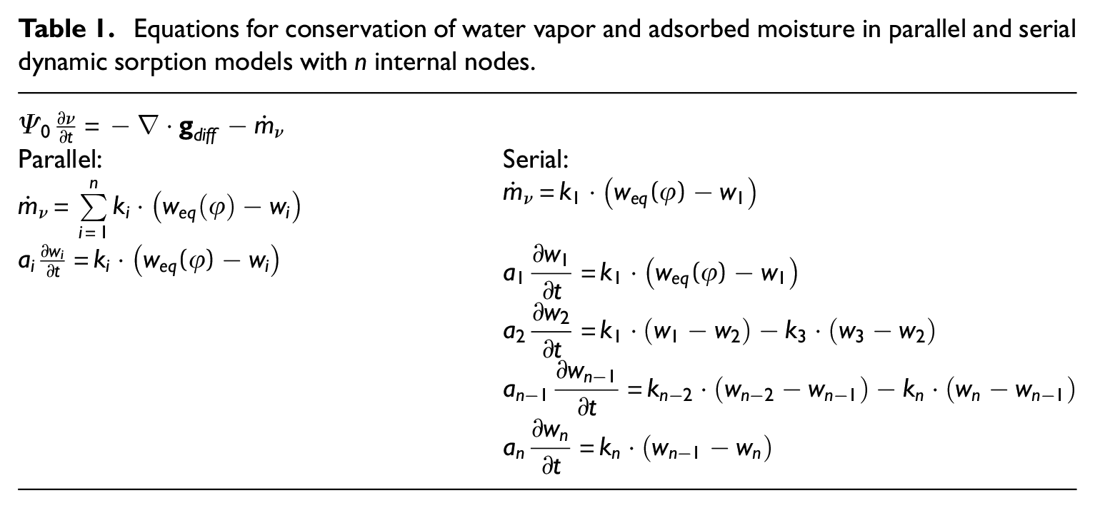
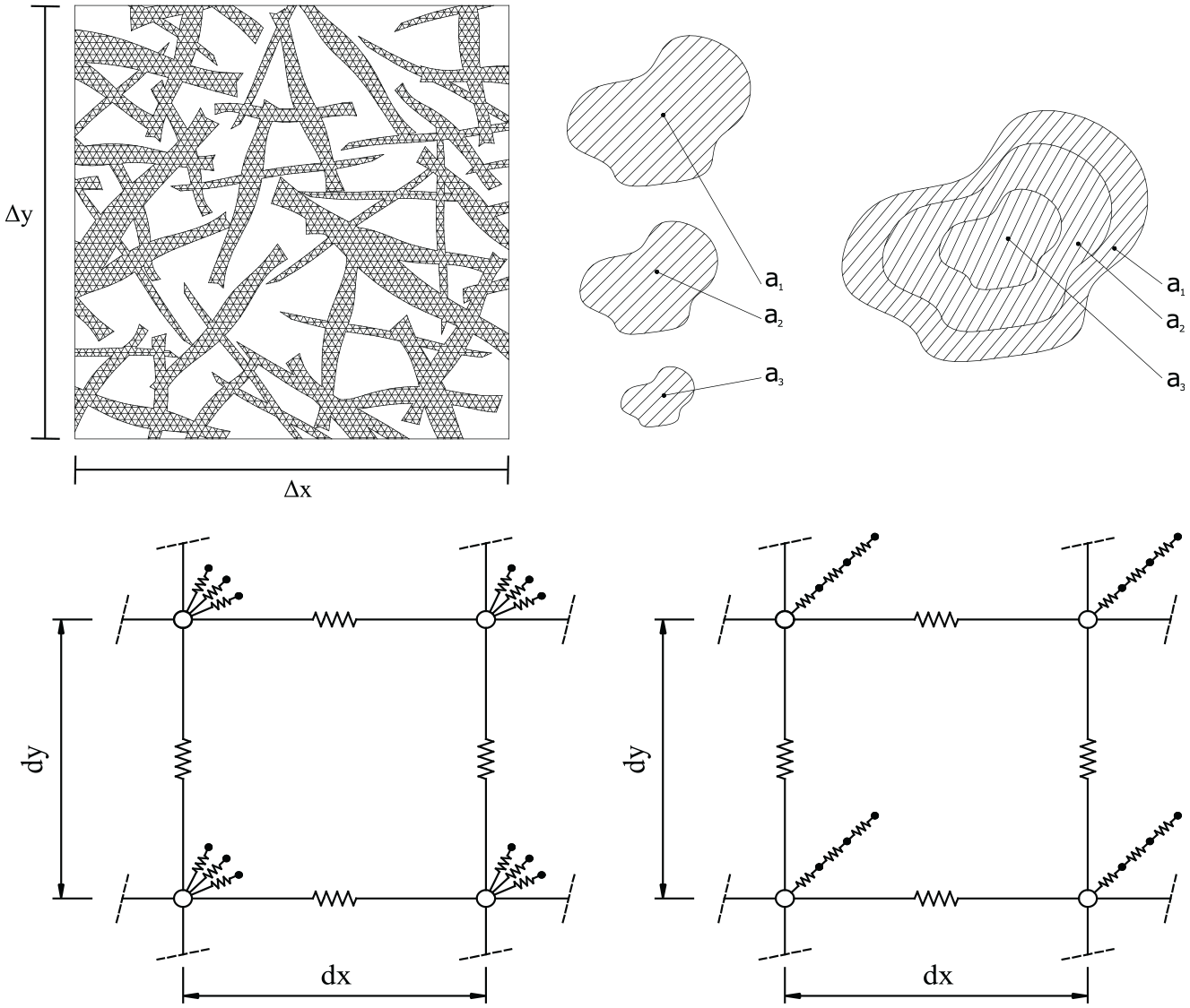
Left, top: Illustration of the wooden strands inside a differential sized representative elementary volume of LDF. Right, top: Illustration of the interpretation of parallel and serial dynamic sorption models with three internal nodes. Bottom: Illustration of the mathematical connections in parallel (left) and serial (right) models.

A sorption balance (also called dynamic vapor sorption analyzer (DVS)) manufactured by Surface Measurement Systems Ltd. was used (model: DVS 1 Adventure) to obtain empirical data for the dynamic sorption behavior of LDF-material. Purpose of such DVS-devices is to record gravimetric data with highly accurate microbalance during hygrothermally dynamic processes, where the sorption rate in a small sample changes. Such devices are also suitable for the study of wood and wood-based materials (Naderi et al., 2016). 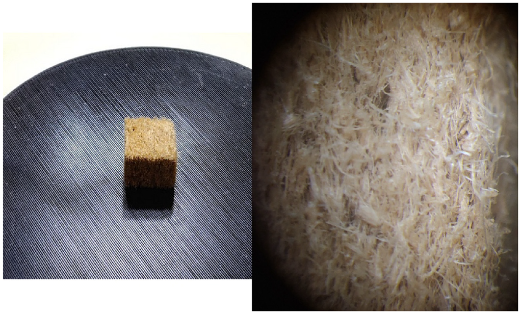Sample is held in a weighing pan, which is located in a chamber, where air flows around it (200 $c m^{3} / \min$ ) and the air temperature and humidity are controlled accurately. In this study we used constant temperature (20 $° C$ ) and subjected small LDF sample (mass roughly 30 mg, size 5 × 5 × 5 mm) to different step changes in relative humidity. Two photographs of the material are shown in Figure 2 (cube-shaped block in the left photo is larger than what was used in the DVS-tests). Illustration of the DVS analyzer’s system schematic and photographs of the equipment are shown in Figure 3.

Figure 2.

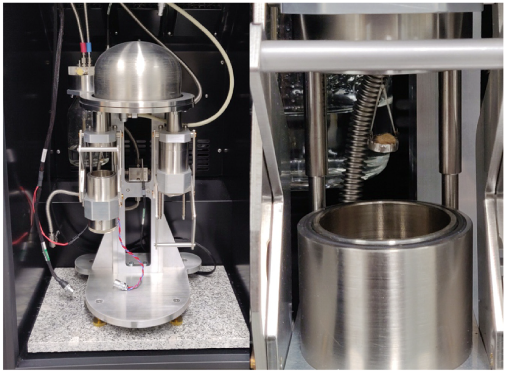
Left: A block (approximately 1 $c m^{3}$ of LDF on a small microscope plate. Right: Photograph of the material through low magnification optical microscope.

Figure 3.

Left: Microbalance and the sample and reference chambers inside the equipment’s incubator. Right: Sample in a weighing pan in the sample chamber, hanging from the microbalance.

Average density of the material is 280 $kg / m^{3}$ as reported by the manufacturer. As can be seen from the photographs, LDF consists of thin and tortuous wood strands, whose average thickness is difficult to estimate. However, since they are clearly visible with naked eye the strands are much thicker than single tracheids, whose average diameter in Baltic pines is around 30 $μ m$ (Irbe et al., 2013). Because of the thinness and tortuosity of the fibers and the slowness of diffusion in wood cell walls, vapor diffusion in LDF pore air is the only included mechanism for bulk moisture transfer in the models. Parallel and serial models containing 1–3 nodes tested in this study are interpreted as moisture-physical systems, where the fibers are discretized either as finite number of proportions of fibers with certain effective diameters (parallel model) or as finite levels or depths to which the molecules are adsorbed inside the fibers (serial model, see Figure 1).

Parameter estimation

DVS test procedure started by keeping the sample in 0% RH conditions for 12 h to determine the dry mass. Before the test, sample was held for several months in a climate room where temperature and humidity were held almost constant (20 $° C$ , 50% RH). After the initial dry period in the DVS-test, the EMCs ( $w_{eq}$ ) at 50%, 60%, and 70% RH were determined with 12 h steps. After the 70% RH step the sample was kept again in 50% RH for 12 h before the actual dynamic test, which had three phases where the sample was subjected to different 15 min step-changes between the values 50%, 60%, and 70% RH:

Phase 1: Step-changes between 50% RH and 60% RH

Phase 2: Step-changes between 50% RH and 70% RH

Phase 3: Step-changes from 60% RH to 70% RH, back to 60% RH, to 50% RH and back to 60% RH

Data logging interval in the DVS was 10 s.

The parameter estimation in least-squares sense is fundamentally based on the numerously repeated evaluation of the objective function for which we would like to find global minimum and corresponding argument:

F (x) = \sum_{i = 1}^{l} {[Y_{i} - m_{i} (x)]}^{2}

(2)

where

$F (x)$ = Objective function; Sum of the squared discrepancies between measurements and numerical results.

$x$ = Vector containing the material parameters, which determine the computational solution.

$Y_{i}$ = Measured value of the sample mass at time $i$ .

$m_{i} (x)$ = Corresponding computed value at time $i$ .

$l$ = Number of measurements (time-steps).

Evaluation of the objective function requires computation of the solution for the time-dependent problem, where the mass of the sample inside DVS evolves during the test. Equations shown in Table 1 form a system of partial differential equations (PDE), which can be solved numerically. However, numerical solving of such PDE-problem with spatial gradiants is heavy task even for small and simple material sample, if tens or even hundreds of thousands of solutions are required to be obtained in reasonable time for different parameter sets. Therefore, it is necessary to simplify the problem by assuming that the diffusion of water vapor inside the sample is very fast and that the sample behaves like a pointlike object. Mathematical problem reduces thus to an initial value problem governed by a set of ordinary differential equations (ODE), where the time-dependent relative humidity $φ$ inside pores is given and only moisture contents $w_{i}$ need to be solved. All the ODE-solutions were computed by using Python-library Scipy’s (version 1.2.1) function scipy.integrate.solve_ivp with LSODA-algorithm (Jones et al., 2001).

Straightforward approach would be to use some robust optimization method to find parameter set, which minimizes the objective function. The parameter estimation was first attempted by using different population-based derivative-free global optimization methods. Results of these attempts are not elaborated here, but we note that the tried algorithms stuck repeatedly at different local minima, which is problematic and unsatisfactory result. This issue had to be dealt with and the solution was to change the mathematical point of view. Instead of seeking the absolutely best fit, we can seek for the most probable parameter set in light of measurements and a priori knowledge by approximating the posterior probability density defined by the Bayes’ rule:

p (x | Y) \propto p (Y | x) \cdot p_{pr} (x)

(3)

where

$p (x | Y)$ = posterior distribution, that is,, probability density function (PDF) for the parameters $x$ given that we have realized measurements $Y = [Y_{1}, Y_{2}, . . ., Y_{l}]^{T}$

$p (Y | x)$ = likelihood for the measurements $Y$ given that the parameters are $x$

$p_{pr} (x)$ = prior PDF of parameters $x$

In this study we used a simple Gaussian likelihood model, which resembles the least-squares objective function:

p (Y | x) = \exp (- \frac{1}{Z} \sum_{i = 1}^{l} {[Y_{i} - m_{i} (x)]}^{2})

(4)

Z is a variance parameter whose meaning and correct value is discussed later in the paper. The used prior function, $p_{pr} (x)$ , was unity, since we didn’t have much beforehand knowledge even about the order of the magnitude of the parameters. This parameter estimation method is nevertheless based on Bayesian inference of the measurement data since we hard-coded some a priori knowledge of the parameters in the sampling algorithm: The parameters must be non-zero and positive.

Approximation or “drawing” of the posterior probability $p (x | Y)$ was done by using following random walk implementation of Metropolis-Hastings algorithm, which belongs to Markov Chain Monte Carlo methods (MCMC) and is applicable when we cannot compute directly the posterior values, but we can compute values proportional to it (Kaipio and Somersalo, 2005; Liu, 2008):

Pick a start point for $x$ and calculate $f (x)$ (in this case: $p (Y | x)$ ).

Draw a random candidate for a new point, $x' = x + ϵ$ , where $ϵ$ is drawn randomly from $N (0, γ I)$ . Variance $γ$ is chosen by user and it controls the “range of exploration”.

Draw random $u$ from uniform density, $U ([0, 1])$ .

Compute the ratio: $α = f (x') / f (x)$ .

If $α > u$ , accept the $x'$ as new $x$ , store it and go to step 2 (or terminate iterations, if desired amount of accepted steps have been obtained). If $α < u$ , reject $x'$ and go back to step 2.

Here, in principle, $x = [k_{1}, k_{2}, . . ., k_{n}, a_{1}, a_{2}, . . . a_{n}]$ . Based on preliminary numerical experiments we saw that for example, for 1-node model the best fitting value for $k_{1}$ is near $\exp (- 6) \approx 0.0025 1 / s$ . We used logarithmically scaled parameter space for $k$ -parameters and constrained the search within region of interest (ROI): $k_{i}^{*} = [3 . . . 15]$ where $k_{i}^{*} = - \ln (k_{i})$ . The random walk was thus carried out by using: $x = [k_{1}^{*}, k_{2}^{*}, . . ., k_{n}^{*}, a_{1}, a_{2}, . . . a_{n}]$ . The ROI prior was implemented in the algorithm by not allowing the algorithm to propose improper values (random candidates outside of ROI were rejected in the step 2 until a proper candidate was proposed at random). Because of the constraint for a-parameters (see Table 1), writing a suitable proposal function for random candidates for $a_{i}$ required also special attention. New acceptable but randomly proposed value for $a = [a_{1}, a_{2}, . . ., a_{n}]$ can be generated by generating first $n - 1$ random values between 0 and 1. These values are sorted and $a_{dir}^{*}$ is then defined as the spans between 0, 1 and the randomly generated values. This guarantees that the sum of the elements of $a_{dir}^{*}$ is 1. $a_{dir}^{*}$ is generated twice every step and we define the direction for new $a$ as $a_{dir} = a_{dir, 1}^{*} - a_{dir, 2}^{*}$ which guarantees that the sum of the elements of $a_{dir}$ is 0. New values for a-parameters are then generated by normalizing the length of the direction vector $a_{dir}$ and multiplying it with random distance $D$ drawn from $N (0, γ)$ and adding to the previous $a$ :

a' = a + D \cdot \frac{a_{dir}}{| a_{dir} |_{2}}

(5)

Equation (4) is a Gaussian probability density for variables which are independent and identically distributed. In our case, it is obvious that the variables (measured and numerically solved masses of the sample) for different time-steps are not independent and some complex covariance structure exists over the whole time span under inspection. Application of Gaussian likelihood is thus, strictly speaking, theoretically unjustified, but because of the overwhelming complexity related to the cumulativeness of the variables, theoretically exact likelihood model is very difficult to derive. However, in this type of time-dependent inverse problem the Gaussian likelihood model may produce useful results and it has been previously used successfully in similar time-dependent parameter estimation problems for differential equations in the studies of for example, chemical reaction rates and systems biology as presented in Girolami (2008) and Pullen and Morris (2014).

The results from parameter estimation implemented in Python were finally used in new FEM-simulations of previously performed laboratory work originally reported in Vinha (2007) and analyzed further in Laukkarinen and Vinha (2011). The structure consisted of following layers from inside to out:

Gypsum board, 13 mm

Bituminous paper

Cellulose-insulation, 173 mm

LDF-board (sheathing), 25 mm

Strong dynamic sorption behavior in local non-equilibria in the sheathing has been previously speculated as one possible cause for the poor agreement between numerical results and relative humidity measurements (Vaisala HMP233) from the interface between LDF-board and thermal insulation layer. Due to lack of space the numerous details related to the modeling of the structure cannot be elaborated here in all details. Structure was modeled as 1D-geometry in Comsol Multiphysics with 85 quadratic elements and using 900 s as maximum limit for the time-steps. The dynamic sorption models were applied by using Coefficient form PDE module for the sheathing domain (dynamic models) and the built-in Building Materials -module for the rest of the domains. Same material properties and boundary conditions were used as in Laukkarinen and Vinha (2011), except the liquid water transport in the sheathing was neglected. In Figure 4 is shown illustration of the building physical research equipment (left) and the time-dependent conditions in the test program used in the laboratory test.

Figure 4.

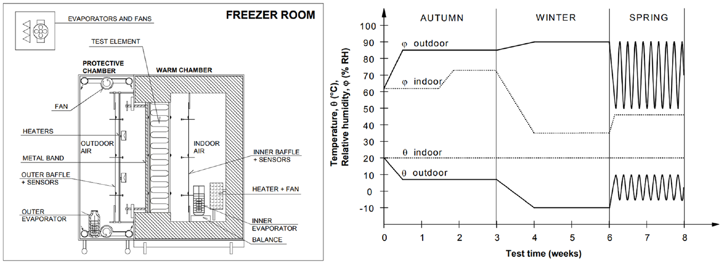
Left: Illustration of the building physical research equipment (Vinha, 2007). Right: Time-dependent temperature and humidity conditions used in the building physical equipment test program.

Results

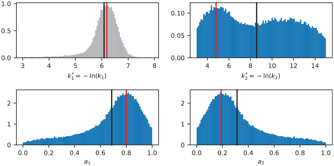
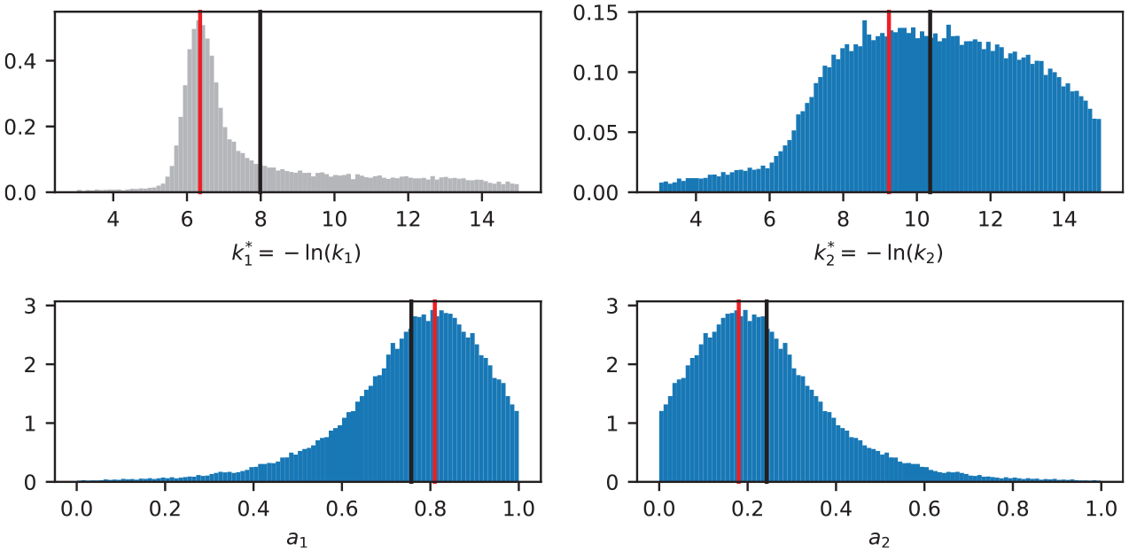
For the 2- and 3-nodes models the random walk sampling was carried out more than once using the information obtained from the first sampling as a new prior knowledge in the later samplings, which are referred to as refined samplings. By samples in this context we mean the points visited by the random walk and by sampling the random walk process of collecting enough samples to draw the distribution. Results for 1-node model parameter samples are shown in Figure 5. Examples of the results from initial independent samplings of 2-nodes serial model are shown in Figures 6 and 7. Figures show normalized histograms of the visited points in the parameter space by the random walks, and they are interpreted as the approximations of marginal probability density functions of the studied parameters, that is, posterior probabilities for individual parameters when other parameters related to the same model are not known.

Figure 5.

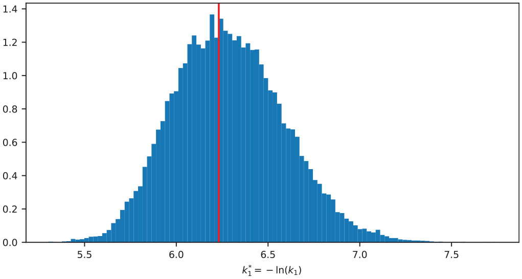
Normalized marginal density for 1-node model parameter. MAP estimate for $k_{1} =$ 0.001967 1/s ( $k_{1}^{*}$ = 6.23).

Figure 6.

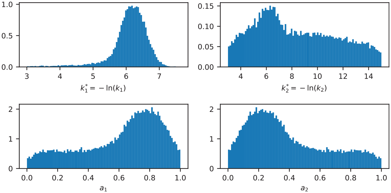
Normalized marginal densities for 2-nodes serial model parameters (Initial sampling, example 1).

Figure 7.

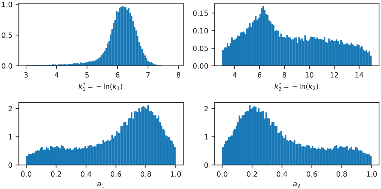
Normalized marginal densities for 2-nodes serial model parameters (Initial sampling, example 2).

Maximum value of the marginal density is defined as the maximum a posterior estimate (MAP) of the parameter (shown with red vertical line in the later figures) and “center of gravity” of the marginal density is the conditional mean estimate (CM, shown with black vertical line in the later figures). Although the marginal densities have distinctive shapes, the approximation contains some saw-edgedness due to numerical imperfections, which are inherently related to Monte Carlo methods. However, the final results and related histograms were visually judged to be smooth enough in order to apply the meaningful computations of MAP and CM estimates. MAP estimates were assessed by fitting 10-degree polynomial to the marginal densities and solving maximum value from the polynomial fit. This can be seen in for example, Figure 5 where the red vertical line (MAP estimate) does not pass through the visibly highest peak in the distribution.

There are no unambiguous rule for which estimate is better in general in inverse problem solutions (Kaipio and Somersalo, 2005). All the random walks presented in this paper were computed independently five times in parallel and the resulting distributions were inspected visually. Because of the lack of space we cannot show all the results, but by comparing Figures 6 and 7 we can see that the random walker obviously reached similar distributions with 100,000 iterations. The used range of exploration parameter for the log-scaled $k^{*}$ -parameters was $γ = 1.0$ and for a-parameters $γ = 0.1$ . These parameters were determined by doing preliminary computational experiments with the random walks and were chosen so that the accept/reject-rate (AR) in the Metropolis-Hastings algorithm would be 0.25...0.35, which is a rule of thumb for suitable AR so that the random walk steps are large enough to cover the whole search space, but not too large so that possibly complex regions in the search space will be also studied densely (Kaipio and Somersalo, 2005).

Realized AR-rates in all the initial samplings were 27.5% on average (from 25.9% to 29.5%), but in the refined samplings, using same range of exploration -parameters they were typically much higher, over 50% in some cases. A standard procedure in the random walk implementations is to throw away certain number of first iterations, since they do not likely represent well the final stationary distribution (Liu, 2008). First 5000 accepted steps were rejected as the “burn-in sequence”. This means that the histograms for marginal densities in the initial samplings are drawn from approximately 20,000–25,000 accepted steps. Total number of steps before algorithm termination was 100,000.

Value used for the variance parameter Z was 1.0 in all computations. If the variables in equation (4) were truly independent and identically distributed, the value of Z should be equal to $2 \cdot σ^{2}$ , where $σ$ is the standard deviation of the measurement error. In this case, the measurement error of the DVS-analyzer’s balance is in the order of magnitude of micrograms (the values in the objective function is milligrams). Smaller values for Z were tried, but it was seen quickly that the random walker cannot get practically any acceptable proposal steps, if there is such small value for Z in the likelihood function. We interpret this finding so, that when using Gaussian likelihood model for time-dependent objective function, the variance parameter Z requires similar trial-and-error experimenting like when choosing suitable range of exploration-parameters for the random walk sampling.

In Figure 8 are shown the marginal densities for parameters obtained by initial random walk sampling for 3-nodes parallel model. The resulting distributions are logical and expected, since the parallel nodes behave all equally. In Figures 9 and 10 are shown the results from refined sampling of 2-nodes serial and parallel models and in Figure 11 are shown the results from refined sampling of 3-nodes parallel model. The value for $k_{1}$ is not sampled any more in the refined sampling (distribution from initial sampling is shown in gray) and the MAP estimate was used while samples for three other parameters were drawn by the random walker (sampling). The resulting distributions from the refined samplings are quite similar to the initial sampling, but more smooth. Pairwise 2D marginal density plots of initially sampled parameters from 2-nodes and 3-nodes serial models are shown in Figures 12 and 13. From the figures can be seen that the posterior distributions may be multimodal, that is, have several local maxima, where different global optimization algorithms may get permanently stuck before finding the globally optimal point in the parameter search space. Also, from Figure 13 can be seen that the deeper nodes we are interested in, the more difficult it is to obtain information from data, which consists of only total weights of material sample at different time-steps. The resulting values for MAP and CM estimates from all the samplings are shown in Tables 2 –5.

Figure 8.

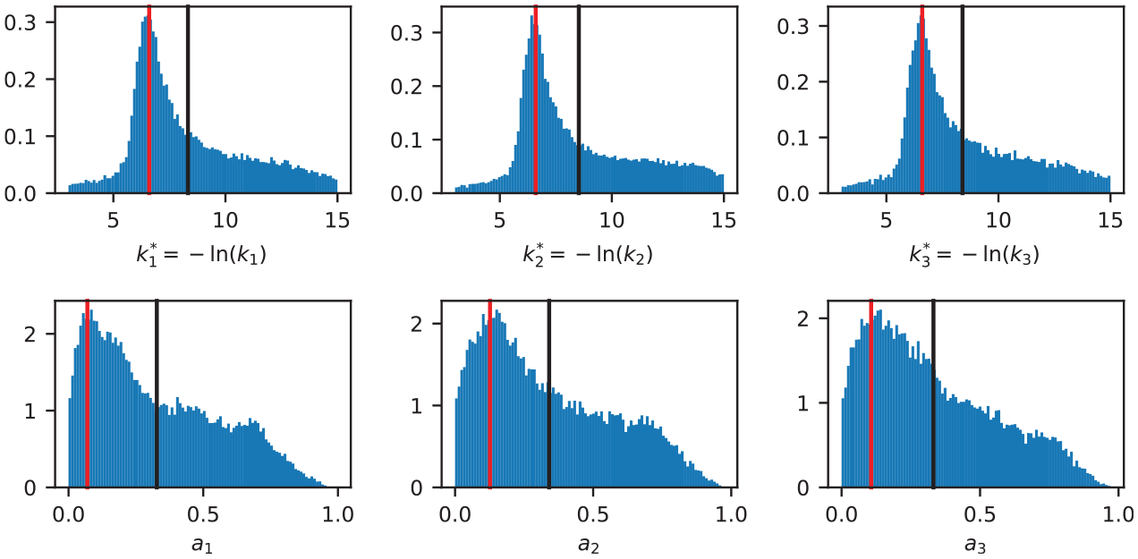
Normalized marginal densities for 3-nodes parallel model (initial sampling).

Figure 9.

Normalized marginal densities for 2-nodes serial model (refined sampling).

Figure 10.

Normalized marginal densities for 2-nodes parallel model (refined sampling).

Figure 11.

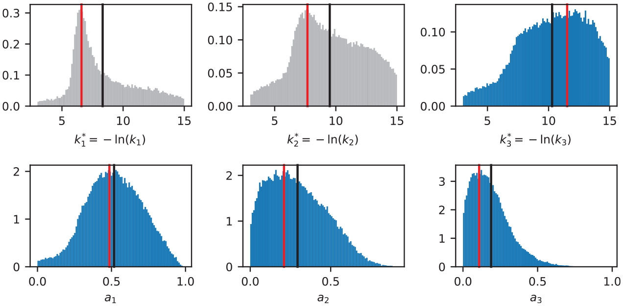
Normalized marginal densities for 3-nodes parallel model (refined sampling).

Figure 12.

Pairwise 2D marginal density plots of the parameters of 2-nodes serial model (initial sampling).

Figure 13.

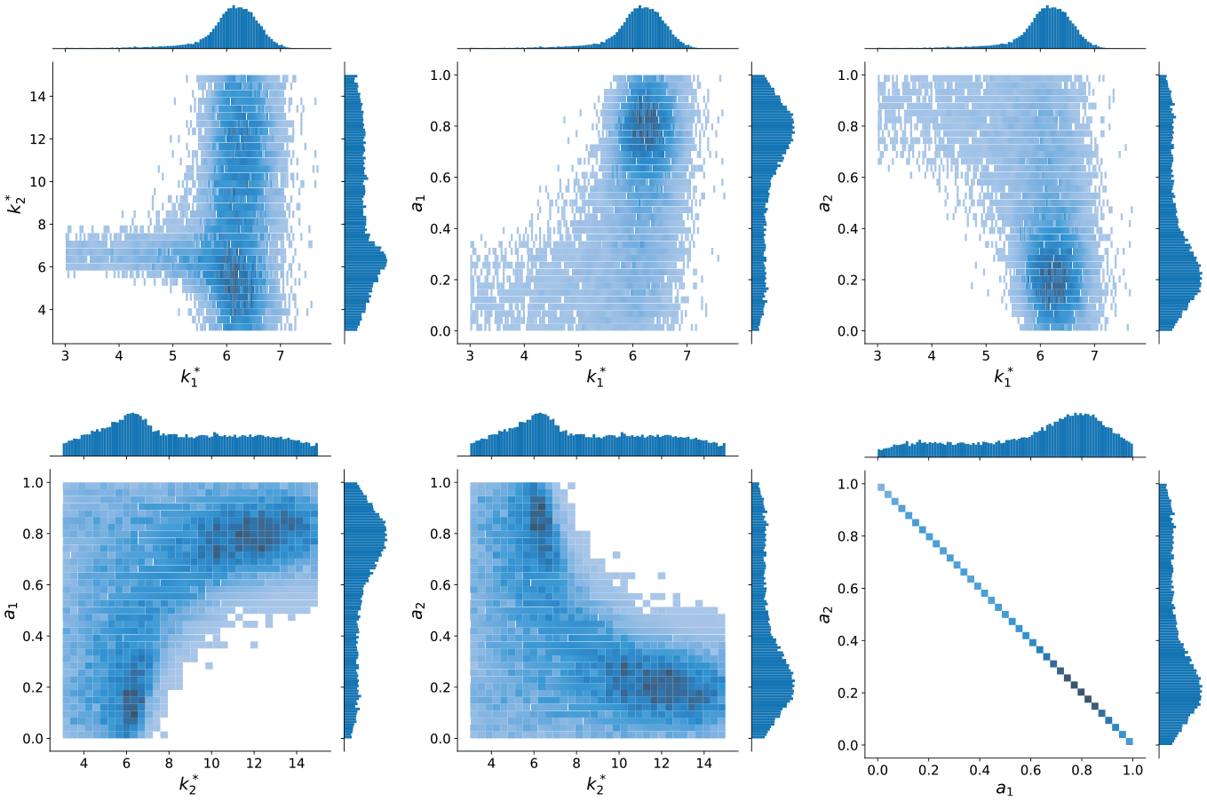
Pairwise 2D marginal density plots of the parameters of 3-nodes serial model (initial sampling).

Table 2.

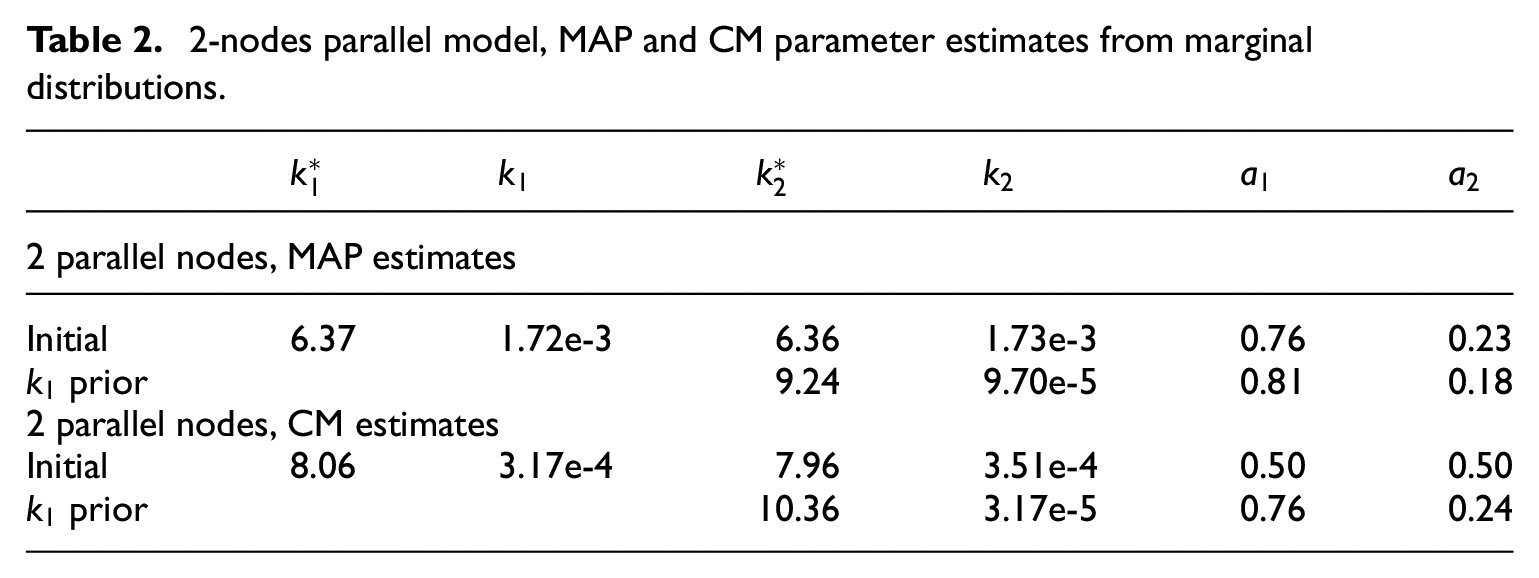
2-nodes parallel model, MAP and CM parameter estimates from marginal distributions.

	$k_{1}^{*}$	$k_{1}$	$k_{2}^{*}$	$k_{2}$	$a_{1}$	$a_{2}$
2 parallel nodes, MAP estimates
Initial	6.37	1.72e-3	6.36	1.73e-3	0.76	0.23
$k_{1}$ prior			9.24	9.70e-5	0.81	0.18
2 parallel nodes, CM estimates
Initial	8.06	3.17e-4	7.96	3.51e-4	0.50	0.50
$k_{1}$ prior			10.36	3.17e-5	0.76	0.24

Table 3.

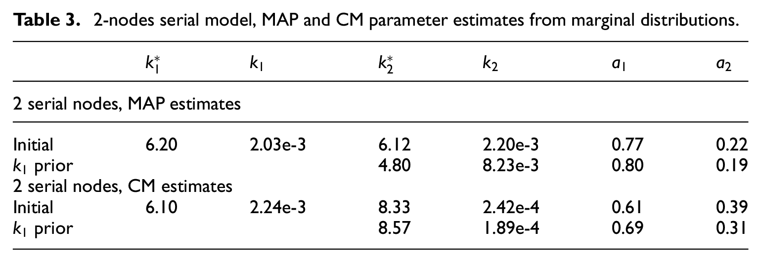
2-nodes serial model, MAP and CM parameter estimates from marginal distributions.

	$k_{1}^{*}$	$k_{1}$	$k_{2}^{*}$	$k_{2}$	$a_{1}$	$a_{2}$
2 serial nodes, MAP estimates
Initial	6.20	2.03e-3	6.12	2.20e-3	0.77	0.22
$k_{1}$ prior			4.80	8.23e-3	0.80	0.19
2 serial nodes, CM estimates
Initial	6.10	2.24e-3	8.33	2.42e-4	0.61	0.39
$k_{1}$ prior			8.57	1.89e-4	0.69	0.31

Table 4.

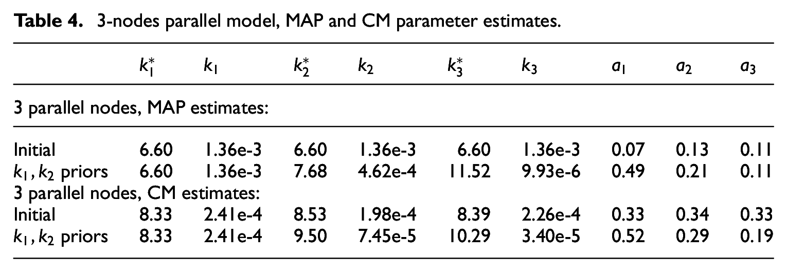
3-nodes parallel model, MAP and CM parameter estimates.

	$k_{1}^{*}$	$k_{1}$	$k_{2}^{*}$	$k_{2}$	$k_{3}^{*}$	$k_{3}$	$a_{1}$	$a_{2}$	$a_{3}$
3 parallel nodes, MAP estimates:
Initial	6.60	1.36e-3	6.60	1.36e-3	6.60	1.36e-3	0.07	0.13	0.11
$k_{1}, k_{2}$ priors	6.60	1.36e-3	7.68	4.62e-4	11.52	9.93e-6	0.49	0.21	0.11
3 parallel nodes, CM estimates:
Initial	8.33	2.41e-4	8.53	1.98e-4	8.39	2.26e-4	0.33	0.34	0.33
$k_{1}, k_{2}$ priors	8.33	2.41e-4	9.50	7.45e-5	10.29	3.40e-5	0.52	0.29	0.19

Table 5.

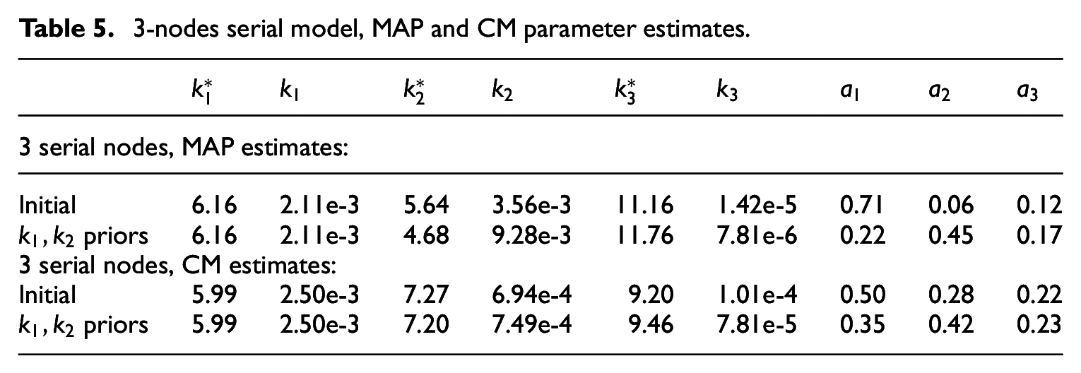
3-nodes serial model, MAP and CM parameter estimates.

	$k_{1}^{*}$	$k_{1}$	$k_{2}^{*}$	$k_{2}$	$k_{3}^{*}$	$k_{3}$	$a_{1}$	$a_{2}$	$a_{3}$
3 serial nodes, MAP estimates:
Initial	6.16	2.11e-3	5.64	3.56e-3	11.16	1.42e-5	0.71	0.06	0.12
$k_{1}, k_{2}$ priors	6.16	2.11e-3	4.68	9.28e-3	11.76	7.81e-6	0.22	0.45	0.17
3 serial nodes, CM estimates:
Initial	5.99	2.50e-3	7.27	6.94e-4	9.20	1.01e-4	0.50	0.28	0.22
$k_{1}, k_{2}$ priors	5.99	2.50e-3	7.20	7.49e-4	9.46	7.81e-5	0.35	0.42	0.23

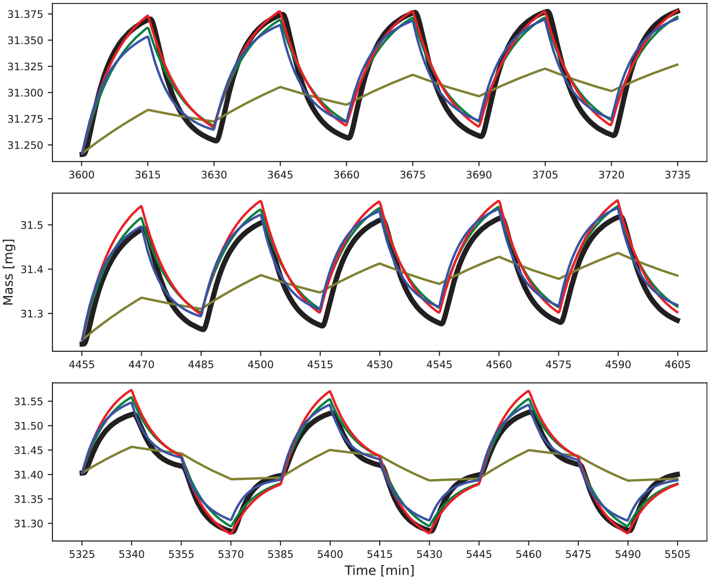
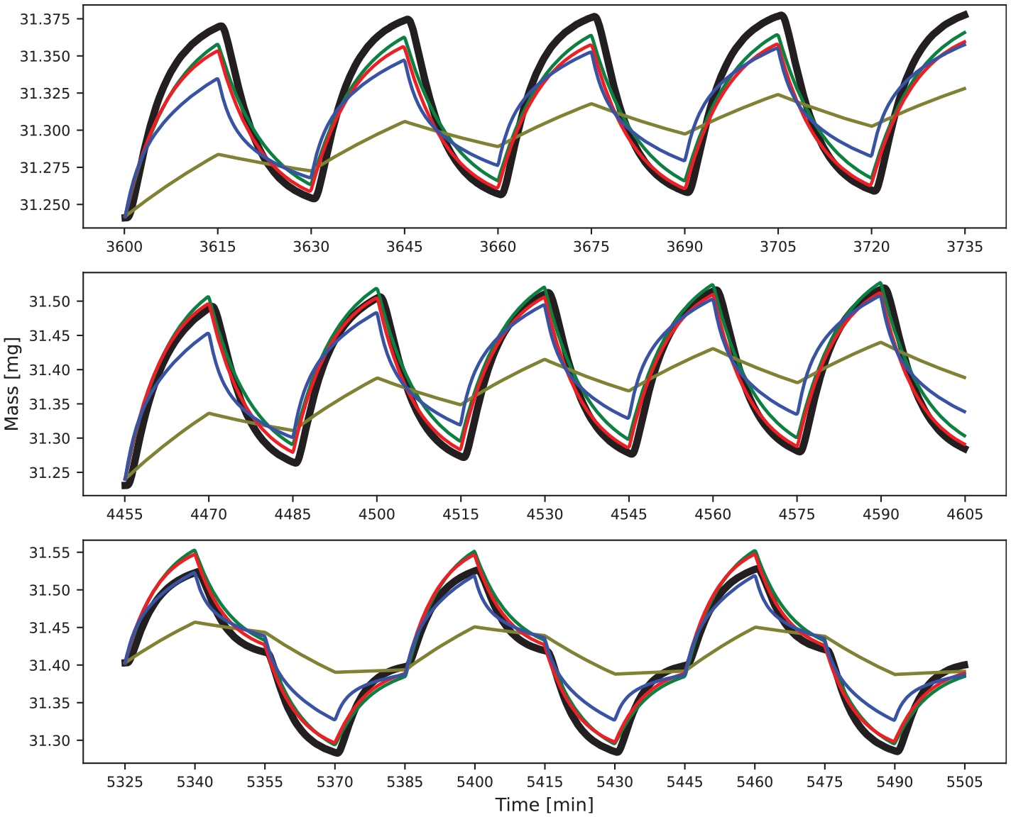
In Figures 14 and 15 are shown the time-dependent curves of the three-phase DVS-tests: the measured masses and numerically solved masses while using different dynamic sorption models and different parameter estimates (MAP and CM). The most obvious observation is that the CM estimate for both 2- and 3-node parallel models (dark yellow line) is a poor choice. In the large area of different types of inverse problems the CM estimate is often characterized as more robust than MAP (Kaipio and Somersalo, 2005), but clearly in this case, MAP estimate is better since the consideration of long tails in the distributions seem to distort the estimation rather than improve it. In Figure 16 are shown also the relative humidity in the DVS, measured masses and numerical results from the dynamic sorption models (only MAP estimates) applied in the PDE-simulation of the sample as a cube in Comsol Multiphysics. As a comparison, results from model using local equilibrium (LE) assumption are also shown. From the results can be easily seen that the dynamic sorption models are clearly better than LE model when modeling numerically the small sample, and that the effect of vapor diffusion is relatively small for the tested sample, since the modeled results from pointlike models and cube models are both close to the measurements. A cautious conclusion may be drawn at this point that because numerical models predict faster mass change rates than measured in test phase 2 (step-changes between 50% and 70% RH) and on the other hand numerical models predict slower mass change rates in test phase 1 (step-changes between 50% and 60% RH), the intrusion of water molecules becomes the slower the more the fibers have already adsorbed moisture. This may mean that instead of—or in addition to—discretizing the moisture capacity into several nodes it may be necessary to introduce also new coefficients, which describe the moisture content dependency of the sorption rate parameters.

Figure 14.

Measurements (black) of the sample mass and corresponding 2-nodes model ODE-solutions in DVS-test. Green = Parallel nodes (MAP), Olive = Parallel nodes (CM), Red = Serial nodes (MAP) and Blue = Serial nodes (CM).

Figure 15.

Measurements (black) of the sample mass and corresponding 3-nodes model ODE-solutions in DVS-test. Green = Parallel nodes (MAP), Olive = Parallel nodes (CM), Red = Serial nodes (MAP) and Blue = Serial nodes (CM).

Figure 16.

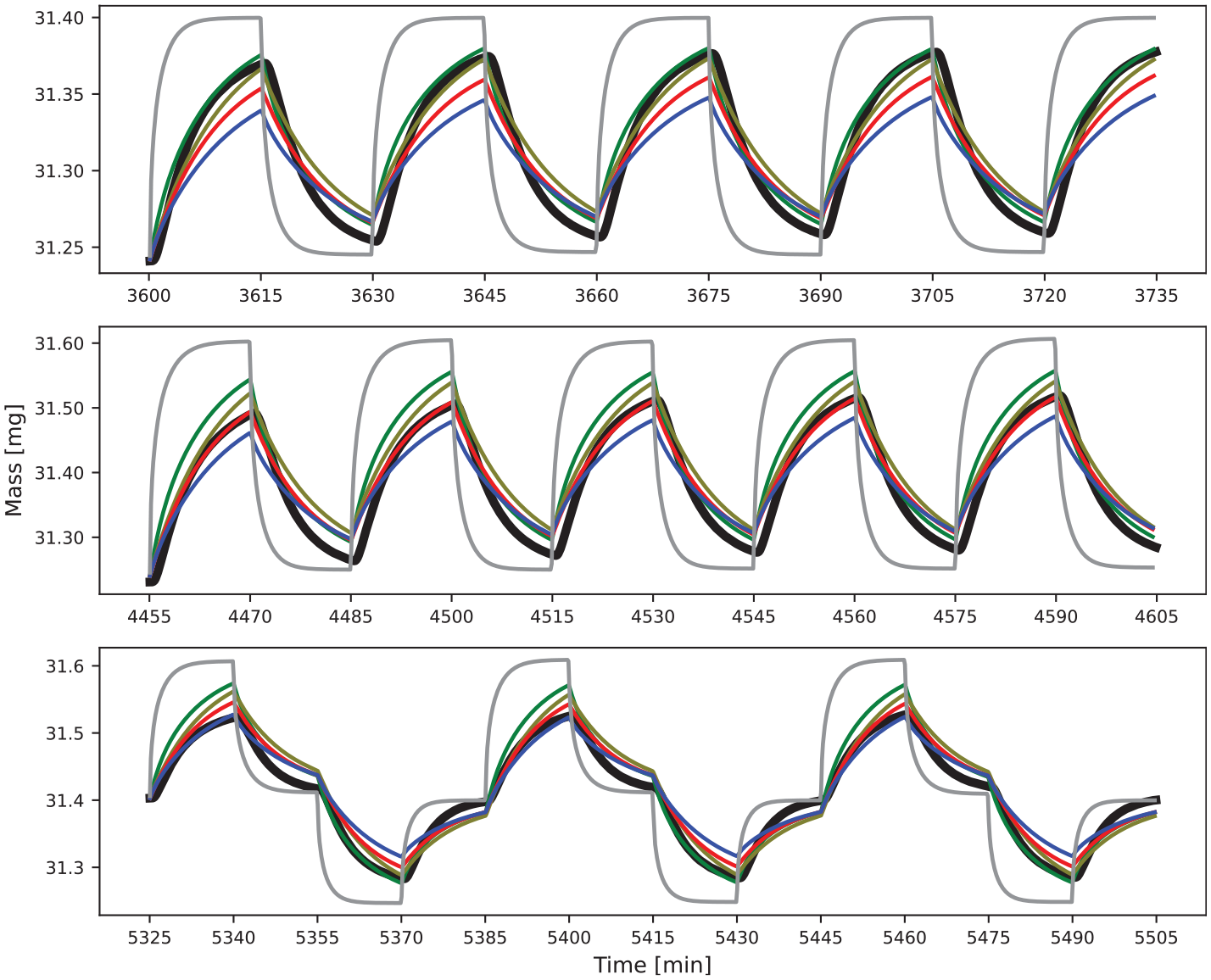
Measurements (black) of the sample mass and corresponding PDE-solutions (cube model in Comsol, MAP estimates used in dynamic sorption models) in DVS-test. Grey = Local equilibrium model, Green = 2 parallel nodes, Olive = 2 serial nodes, Red = 3 parallel nodes and Blue = 3 serial nodes.

In Figures 17 to 19 are shown the results of the modeling of old laboratory test wall. Reference point, which the curves describe, is the interface between LDF-sheathing and insulation layer. With 1-node model the modeling was done with using MAP estimate for sorption rate coefficient and, for the sake of curiosity, with smaller arbitrary values also. In general, the dynamic sorption models seem to improve the agreement between measurements and numerical modeling, but only very slightly, and the results are still not at satisfactory level. Toward the end of the spring phase of the test conditions the measured relative humidity show stronger diurnal fluctuation than any of the simulations—except for the 1-node model where an arbitrarily small and probably unrealistic value for sorption rate coefficient (k = 1e-6) was used. Not much more can be concluded from the laboratory wall simulations, since the test structure contained also cellulose insulation material, which may due to cellulosic origin have also dynamic sorption characteristics. More experimental work is required in order to evaluate the suitability, necessity or usefulness of the studied dynamic sorption models in numerical analyses of real-scaled structures.

Figure 17.

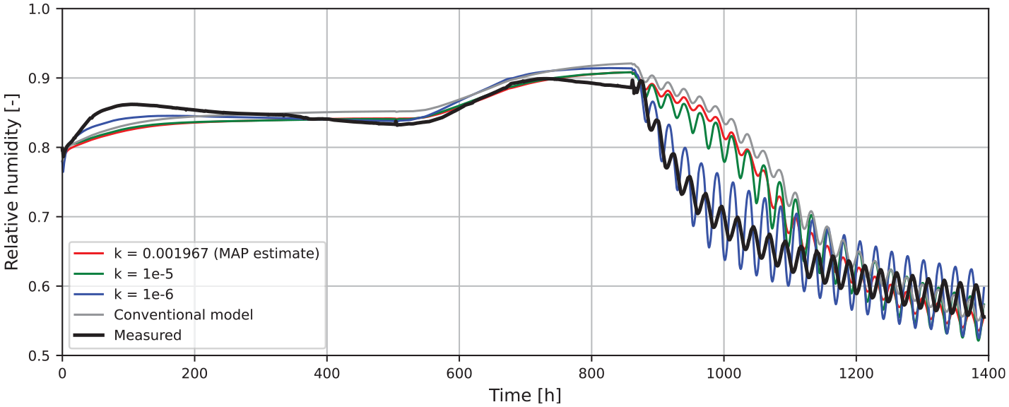
Relative humidity in the reference point of old laboratory test wall according to the measurements and 1-node model with different parameters.

Figure 18.

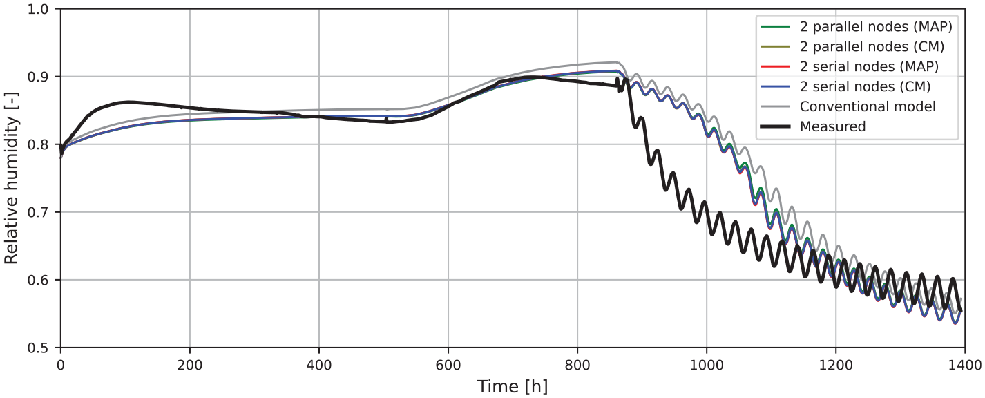
Relative humidity in the reference point of old laboratory test wall according to the measurements and 2-node models with different parameters.

Figure 19.

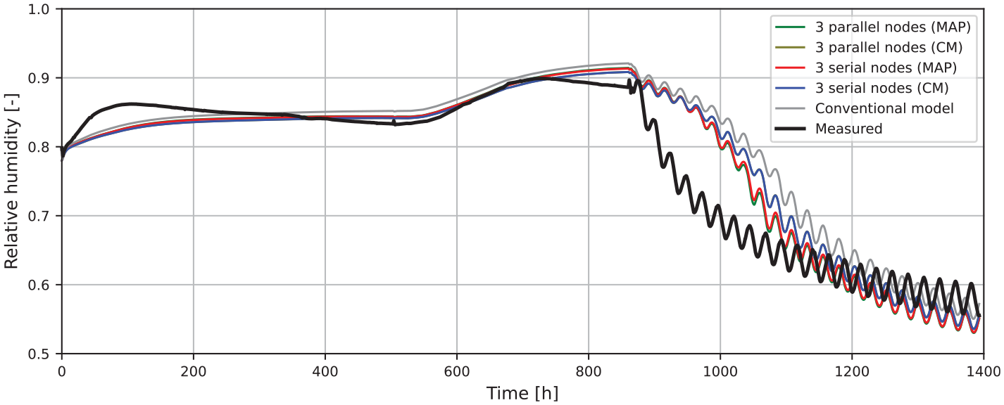
Relative humidity in the reference point of old laboratory test wall according to the measurements and 3-node models with different parameters.

Discussion

Dynamic sorption and improving the hygrothermal models for wood and other cellulosic materials is an active topic in research. Different types of mathematical improvements have been proposed in recent years for numerical models. However, introducing several new parameters in the model equations may yield a formidable model fitting problem when the new parameters are attempted to be estimated from time-dependent gravimetric data. In such cases, global optimization approach even with vast computational resources may be ineffective because of the multimodality of the objective function. A more robust approach may be statistical inversion as presented in this paper, which is relatively easy to implement with random walk Metropolis-Hastings algorithm. However, there are certain open questions related to for example, suitable likelihood model and proper effective variance parameter values in the implementation of the algorithm. The statistical inversion method applied in this paper could be possibly useful also in other building physical material studies, where the measurable time-dependent data contains information about certain moisture transfer or storage related parameters, but which are very difficult to solve directly from the measured data.

Conclusions

By comparing the measurements, conventional modeling results and new numerical analyses with dynamic sorption models we can see that essential improvement in the results for the analysis of real-scaled laboratory test wall could not be achieved by using dynamic sorption models for the LDF sheathing board. However, the numerical analysis of the sample studied in the DVS-analyzer show clearly observable slowness in the sorption and the corresponding development of the sample’s mass, which the local equilibrium model fails to predict. These observations may imply that the slowness of sorption in the studied LDF-material is significant enough to be measured and simulated numerically with satisfactory accuracy, but the dynamic effects due to the slowness occur in such small time scales that it may be negligible in many building physical studies, where the conditions change in clearly slower cycles than the 15 min step-changes, which were used in the DVS-tests. However, reason for the poor agreement between modeling and measurements in the old laboratory test assembly inspected in this paper is still unclear. Possible explanatory known moisture-physical phenomena—which were not taken into account in the simulations presented in this paper—are temperature-dependent and hysteretic properties of the sorption isotherm of LDF, which will be a future topic of the authors’ research.

Footnotes

Acknowledgements

We would like to kindly thank prof. Sampsa Pursiainen for his advices on inverse problem techniques.

Declaration of conflicting interests

The author(s) declared no potential conflicts of interest with respect to the research, authorship, and/or publication of this article.

Funding

The research was funded by doctoral school program of Tampere University of Technology (now Tampere University) and has received also general funding from Faculty of Built Environment, Tampere University.

ORCID iD

Petteri Huttunen

References

Absetz

(1999) Moisture transport and sorption in wood and plywood. Theoretical and experimental analysis originating from wood cellular structure. Dissertation, Helsinki University of Technology. Laboratory of Structural Engineering and Building Physics Publications, Espoo, Finland.

Challansonnex

Casalinho

Perré

(2019) Non-Fickian diffusion in biosourced materials: Prediction of the delay between relative humidity and moisture content. Energy and Buildings 202: 109340.

Defo

Lacasse

Laouadi

(2022) A comparison of hygrothermal simulation results derived from four simulation tools. Journal of Building Physics 45(4): 432–456.

Engelund

Klamer

Venås

(2010) Acquisition of sorption isotherms for modified woods by the use of dynamic vapour sorption instrumentation. Principles and practice. In: 41st annual meeting of the international research group on wood protection, Biarritz, France, IRG SECRETARIAT, Box 5609, SE-114 86 Stockholm, Sweden. www.irg-wp.com, p.10.

Girolami

(2008) Bayesian inference for differential equations. Theoretical Computer Science 408(1): 4–16.

Håkansson

(1998) Retarded sorption in wood. Experimental study, analyses and modelling. Report TABK–98/1012, Department of Building Science, Lund Institute of Technology, Sweden.

Irbe

Sable

Treimanis

, et al. (2013) Variation in the tracheid dimensions of scots pine (Pinus sylvestris L.) and Lodgepole pine (Pinus contorta Dougl. var. latifolia Engelm) trees grown in Latvia. Baltic Forestry 19(1): 120–127.

Janssen

Scheffler

Plagge

(2016) Experimental study of dynamic effects in moisture transfer in building materials. International Journal of Heat and Mass Transfer 98: 141–149.

Jones

Oliphant

Peterson

, et al. (2001) SciPy: Open source scientific tools for Python. Available at: http://www.scipy.org/ (accessed 27 November).

10.

Kaipio

Somersalo

(2005) Statistical and Computational Inverse Problems. Berlin: Springer Science+Business Media, Inc. pp.94–98.

11.

Korjenic

Bednar

(2011) Developing a model for fibrous building materials. Energy and Buildings 43(11): 3189–3199.

12.

Krabbenhøft

(2004) Moisture transport in wood - A study of physical-Mathematical models and their numerical implementation. PhD Thesis, Department of Civil Engineering, Technical University of Denmark, p.105. BYG-Rapport R-153

13.

Künzel

(1995) Simultaneous heat and moisture transport in building components. One- and two-dimensional calculation using simple parameters. Dissertation, Fraunhofer IRB Verlag Suttgart, 1995.

14.

Laukkarinen

Vinha

(2011) Comparison of calculated and measured values of wall assembly tests using Delphin 5. In: Vinha

Piironen

Salminen

Proceedings of the 9th Nordic Symposium of Building Physics, NSB 2011, Tampere, Finland, vol.1, pp. 155–162. Department of Civil Engineering, Tampere University of Technology.

15.

Liu

(2008) Monte Carlo Strategies in Scientific Computing. Berlin: Springer Publishing Company, Incorporated.

16.

Metsäntutkimuslaitos Metla (Finnish Forest Research Institute) (2012) State of Finland’s Forests 2012: Criterion 4 Biological Diversity. Natural Resources Institute Finland(Luonnonvarakeskus Luke), viewed 9. February 2021. Available at: http://www.metla.fi/metinfo/sustainability/c4-tree-species.htm (accessed 19 December 2022).

17.

Naderi

Acharya

Cattaneo

, et al. (2016) Analysis of wood and biomaterials by dynamic vapor sorption technique. In: Hansen

Rode

Nilsson

(eds.) Proceedings of the international RILEM conference. Materials, Systems and Structures in Civil Engineering 2016, Segment on Moisture in Materials and Structures, Lyngby, Denmark, 22–24 August 2016, pp.51–58. Technical University of Denmark, RILEM Publications S.A.R.L., 4 avenue du Recteur Poincare, 75016 Paris - France.

18.

Ojanen

Viitanen

Peuhkuri

, et al. (2010). Mould growth modeling of building structures using sensitivity classes of materials. In: Proceedings of Thermal Performance of the Exterior Envelopes of Whole Buildings XI International Conference. Thermal Performance of the Exterior Envelopes of Whole Buildings XI, Buildingx XI Conference - Clearwater Beach, Florida, United States, 5–9 Nov 2010, ASHRAE. https://pdfs.semanticscholar.org/8830/641d0ac664ccc0afb5f84351d24fd3386b66.pdf (Accessed December 19, 2022).

19.

Pullen

Morris

(2014) Bayesian model comparison and parameter inference in systems biology using nested sampling. PLoS One 9(2): e88419.

20.

Rowell

(2013) Handbook of Wood Chemistry and Wood Composites, 5th edn. Boca Raton, FL: CRC Press.

21.

Saeidpour

Wadsö

(2015) Evidence for anomalous water vapor sorption kinetics in cement based materials. Cement and Concrete Research 70: 60–66.

22.

Skaar

(1988) Moisture movement in the wood cell wall. In: Timell T.E. (ed.) Wood-Water Relations. Springer Series in Wood Science. Berlin: Springer-Verlag Berlin Heidelberg, p.283.

23.

Telkki

V-V

Yliniemi

Jokisaari

(2013) Moisture in softwoods: Fiber saturation point, hydroxyl site content, and the amount of micropores as determined from NMR relaxation time distributions. Holzforschung 67: 291–300.

24.

Thybring

Glass

Zelinka

(2019) Kinetics of water vapor sorption in wood cell walls: State of the art and Research needs. Forests 10(8): 704.

25.

Vinha

(2007) Hygrothermal performance of timber-framed external walls in finnish climatic conditions: A method for determining the sufficient water vapour resistance of the interior lining of a wall assembly. Dissertation. Publication 658, Tampere University of Technology, pp.338 + 10 app. Available at: http://urn.fi/URN:NBN:fi:tty-200903101040 (accessed 19 December 2022).

26.

Vinha

Käkelä

(2000) Water vapour transmission wall structures due to diffusion and convection. Publication 103. Tampere University of Technology, Structural Engineering. p.110. Available at: http://urn.fi/URN:ISBN:978-952-15-3159-0 (accessed 19 December 2022).

27.

Wiemann

(2010) Characteristics and Availability of Commercially Important Woods. In: Ross

Robert J.

(ed.) Wood Handbook - Wood as an Engineering Material, Madison, Wisconsin, Chapter 2, page 1., United States Department of Agriculture Forest Service. USA: Forest Products Laboratory.

28.

Yamamoto

Takada

(2022) Influence of variability in hygrothermal properties on analytical results of simultaneous heat and moisture transfer in porous materials. Journal of Building Physics 45(6): 757–773.

Dynamic water vapor sorption in wood-based fibrous materials and material parameter estimation

Abstract

Keywords

Introduction

Background: Moisture storage and sorption in wood

Materials and methods

Parameter estimation

Results

Discussion

Conclusions

Footnotes

Acknowledgements

Declaration of conflicting interests

Funding

ORCID iD

References