
Abstract
Background:
Although the analysis of event-based clinical trials commonly relies on assumptions about the underlying hazard functions, in practice it is rare to see estimates of those functions.
Methods:
I describe conventional and novel methods for estimating the hazard function using discrete and discretized continuous survival models. The conventional approach involves parametric modeling; the novel approach applies Bayesian model averaging to flexible modeling by splines or fractional polynomials. I evaluate the methods in a Monte Carlo study and illustrate them in the analysis of three historical clinical trials.
Results:
Although flexible models can capture features of the hazard functions—such as multimodality—that parametric models miss, they are not foolproof. Spline modeling was generally the most reliable, in the sense of yielding good coverage probabilities for the mean and median with modest loss of efficiency. In the examples, the discreteness of the measurements—days, weeks, or months—had little effect on the shape of estimated hazard functions. All three data sets showed some evidence of departure from the proportional hazards assumption, but in only one did a test for proportionality detect this departure.
Conclusion:
Flexible parametric models, estimated in the Bayesian model averaging framework, offer a robust approach to recovering the shape of the hazard function. Analyses of three clinical trial databases suggest that visualization of the hazard function can be a valuable adjunct to conventional survival analysis.
Introduction
In event-based clinical trials, it is common to base analyses of survival outcomes on the Cox proportional hazards model. 1 The simplifying assumption of proportionality enables deployment of a partial likelihood analysis that avoids estimating the hazard functions. It is typical to interpret the proportionality factor—the hazard ratio—as a treatment effect that measures the relative risk of an event at any point in the follow-up.
Recognizing that proportional hazards is unlikely to hold exactly, statisticians have devised alternative versions of the hazard ratio.2,3 Most significantly, the “Cox model average hazard ratio” is a censoring-dependent parameter that the partial likelihood analysis consistently estimates. It is generally taught that the estimand in a Cox analysis is a hazard ratio function averaged over time.
Graphical analyses of event-based trials typically present the data as a comparison of survival curves. 4 This analysis is reliable and straightforward, because the Kaplan–Meier curve consistently estimates the underlying survival curve under mild assumptions and is readily interpretable. As the survival curve is fully equivalent to the hazard function—in the sense that knowing the survival you can calculate the hazard, and vice versa—there is no theoretical reason to prefer one to the other. Yet despite the common use of the hazard ratio as a touchstone for model-based analysis, it is rare to see estimated hazard functions from clinical trials.
To see why, consider Figure 1, which displays the nonparametric estimate of the hazard function in the medical arm of the REMATCH trial. 5 Spikes occur at event times, with height equal to the fraction of subjects in the risk set who had an event at that time. To extract underlying structure from such graphs, investigators have proposed methods for estimating a smooth hazard function from censored data.6–23 An important early example is the method of Efron, 9 in which one estimates the dependence of the hazard on time by logistic regression on a spline predictor. Alternatively, one can directly smooth the nonparametric hazard function. 19
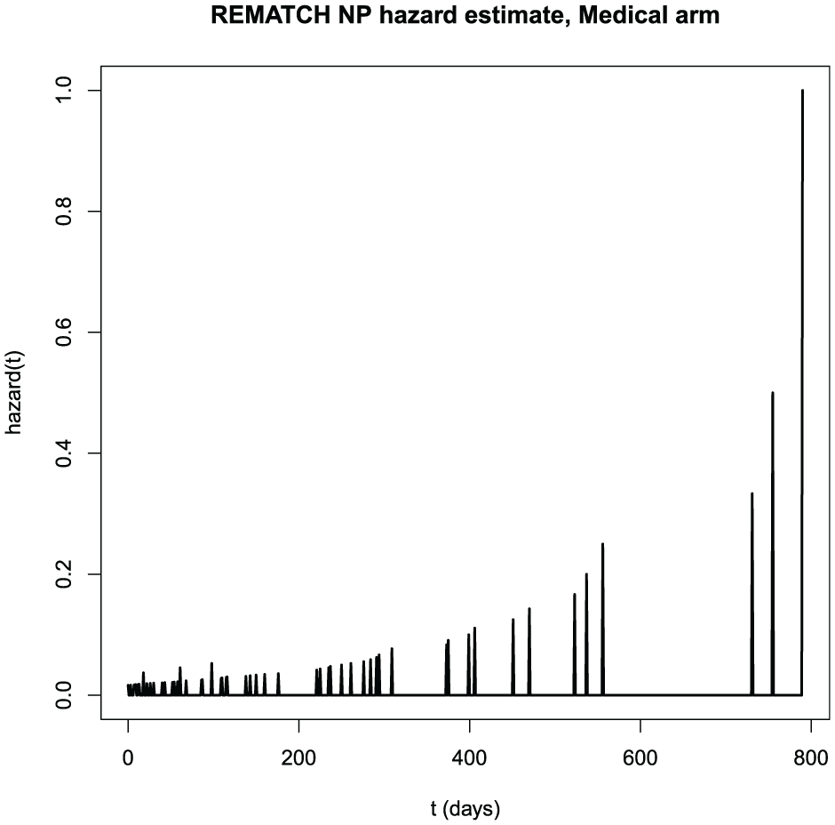
Nonparametric estimate of the hazard function in the medical arm of the REMATCH trial.
Unfortunately, such estimates can be sensitive to spline degree, the placement of knots, and tuning parameters. Thus, model selection is consequential, and measures of variability should properly reflect model uncertainty. Although there are many such estimation methods, including some implemented in popular software, clinical trial applications remain rare.
This article revisits the problem of estimating hazard functions in an event-based clinical trial. I extend Efron’s 9 method by incorporating fractional polynomials,12,17 and I account for model selection by Bayesian model averaging.24,25 In a simulation study, I observe that flexible logistic regression with Bayesian model averaging performs nearly as well as a correctly specified parametric model and better than an incorrectly specified parametric model.
Analyses of three clinical trial examples reveal substantial departures from proportional hazards that significance testing detects in only one.
Methods
Notation
Assume a two-arm clinical trial involving n subjects. The variable
Elements of the statistical model are the hazard function

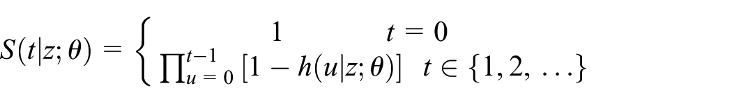
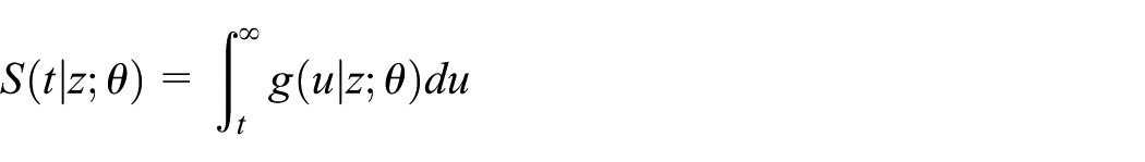
the survival function

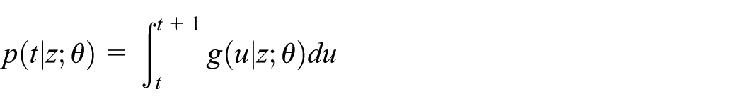
and the probability mass function

all defined on
and the probability mass function as

Here, θ stands for an unknown model parameter.
My definition of the survival function (≥ rather than the usual >) in (1) permits writing the density simply as in (2). Cox 1 (p. 187) also defined the survival function this way.
Standard parametric models
I estimated two kinds of standard parametric models: discrete models and discretized continuous models. With a continuous underlying density
and survival function
for
Flexible parametric models
With discrete survival, it is convenient to model the event hazard at time t by logistic regression.
9
Defining

where
Estimation
Whatever the model, estimation is based on the log-likelihood for right-censored data
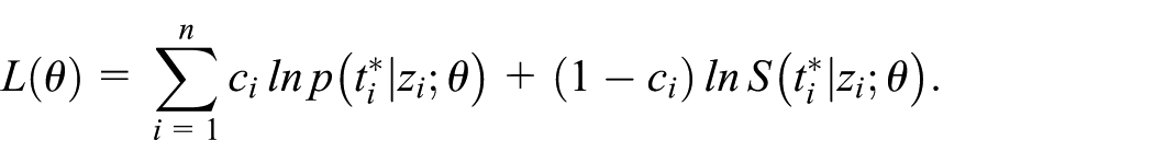
To estimate θ in the parametric models, we maximize
We implement maximum likelihood for the flexible hazard models using Efron’s partial logistic regression,
9
which involves creating, for subject i with survival time
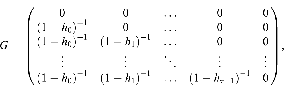
Alternatively, one can create vectors r and d for each arm, where
One computes large-sample standard errors for the hazard and survival ordinates as follows: The variance of the linear predictor is

where W is a diagonal matrix with elements
we get

where
Bayesian model averaging
With flexible modeling, it is challenging to select the spline or fractional polynomial terms to include in the regression. One approach is to choose, from a suitably large family, the model that optimizes a measure of fit such as the Akaike information criterion 26 or Bayesian information criterion (BIC). 27 If one does not account for model selection, standard errors may be too small and significance tests based on model statistics may have size exceeding the nominal.
An alternative in such cases is Bayesian model averaging.24,25 This method involves positing a comprehensive set of models, assigning each a prior probability, estimating each model and computing its posterior probability, and averaging inferences across this posterior. With many types of analyses, the class of potential models is so large that it is impossible to estimate them all. But with flexible parametric regression, even a relatively small set of models—perhaps only a few dozen—should manifest enough shapes to describe any pattern likely to be seen in real data. Thus, one can, with modest effort, conduct an analysis that properly adjusts for model uncertainty.
Once one has estimated each model in the proposed class, the posterior probability of model
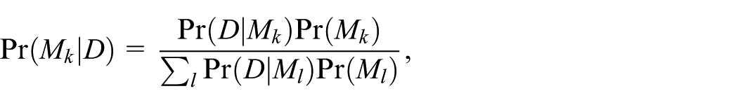
where
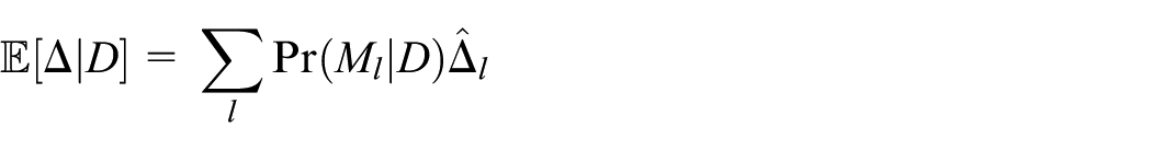
and posterior variance
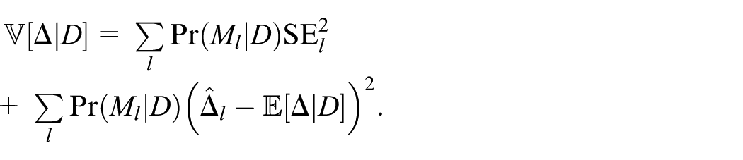
That is, the posterior mean of a parameter is the average of its within-model estimates, and the posterior variance is the average of its within-model variances plus the variance of its within-model estimates, always averaging against the posterior distribution over the models.
For generalized linear models, such as those estimated in flexible modeling by logistic regression, one can approximate
In spline-based analyses, I used a collection of 19 models: An intercept-only model (equivalent to a geometric distribution for discrete data and approximating an exponential for discretized continuous data), and all combinations of models with 0 to 5 knots (at equally spaced quantiles of the observed event times) and linear, quadratic, and cubic terms. I omitted zero-order splines—analogous to the piecewise exponential—because they give non-continuous hazard functions.
With fractional polynomials, I used a collection of 45 models including a null (intercept-only, geometric/exponential); models including an intercept and
Simulation
I conducted a simulation to evaluate frequency properties of the estimation methods in samples of moderate size. I simulated 400 single-arm data sets of size
1. a negative binomial;
2. a discretized exponential;
3. a discretized (non-exponential) Weibull;
4. a discretized lognormal; and
5. a model—henceforth denoted mixture—defined by the bimodal hazard function

where
I chose the exponential distribution to have mean (and standard deviation) 365.25 days, and the other parametric distributions to have mean 365.25 days and standard deviation 400 days. For each data set under each model, I estimated the hazard and the mean and median survival. Because the flexible models had finite support, when computing the mean, I appended an exponential tail beyond the largest t. With independent censoring uniform on 0–36 months (6–36 months for the mixture model), simulations gave on average roughly 70% events.
I computed Wald confidence intervals for mean survival. To obtain an interval for the median, I took as lower confidence bound the smallest t for which the lower limit of the 95% confidence interval of the survival was less than 0.5, and as upper confidence bound the largest t for which the upper limit of the 95% confidence interval was greater than 0.5.
I summarized simulation results by the root mean squared error of estimation and the coverage probability of the 95% confidence interval. With 400 simulations, assuming true 95% coverage probability, the Monte Carlo standard error of the coverage probability estimate is roughly 1%.
Analysis of clinical trial data sets
I applied the flexible methods to data from three historical randomized, event-based trials: REMATCH, 5 the gastric carcinoma trial analyzed by Stablein et al,28,29 and the head-and-neck cancer trial analyzed by Efron. 9 For each trial, I applied both methods to estimate the control and test hazard functions and the hazard ratio as a function of t. To assess the effect of the level of discreteness, I conducted the analysis of each data set with survival in days (the original scale), rounded to the nearest week, and rounded to the nearest month.
Computation
I conducted simulations in R Version 4.5.1 and analyses in R Version 4.5.2. 30
Results
Simulation
Results for mean survival appear in the upper half of Table 1. Coverage probabilities were close to 95% except when one of the generating or analysis models was lognormal. Precision was typically best, or nearly so, under the generating model; again, the lognormal was the exception. The flexible models in most cases had precision somewhat less than the generating model. The spline gave the most precise mean for mixture data.
Simulated coverage probability and root mean squared error for mean and median survival, by generating and analysis model.
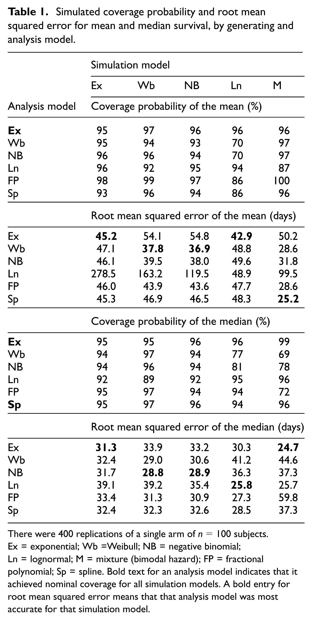
There were 400 replications of a single arm of
Results for median survival appear in the lower half of Table 1. Coverage probabilities were close to 95% except when the simulation model was lognormal or mixture, or the analysis model was lognormal. Precision was best, or nearly so, under the generating model. The flexible models, when calibrated, had precision only slightly less than the generating model, except that the fractional polynomial analysis failed badly for mixture data.
Graphs of averaged estimates of the mixture hazard function (see Supplementary Figures S.1–S.6) reveal that only the spline analysis captures its multiple modes. Figure S.5 shows that the fractional polynomial model underestimated the mixture hazard in the range
Example: REMATCH
The REMATCH trial randomized heart failure patients to receive either optimal medical management or an implantable left-ventricular assist device.
5
Of 129 subjects, 107 experienced events. Analysis by the Cox model gives an estimated hazard ratio of 0.52 (favoring the device) with 95% confidence interval (0.34, 0.78) and logrank
Figure 2 displays the spline estimates of the REMATCH hazard functions. The graph shows an elevated hazard in the device arm at early t, reflecting perioperative mortality from the implantation. The hazard in the control arm is more nearly constant. Figure S.7 displays the REMATCH hazard ratio as a function of time, estimated under the spline model with Bayesian model averaging. The graph suggests the possibility of non-proportional hazards.
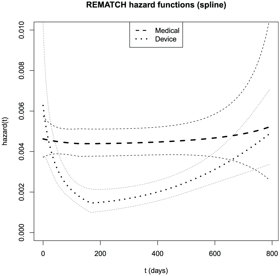
Bayesian model-averaged spline estimates of the REMATCH hazard functions with pointwise standard error bars (
Example: gastric carcinoma
The Gastrointestinal Tumor Study Group conducted a randomized trial comparing chemotherapy alone to chemotherapy plus external radiotherapy in locally advanced gastric carcinoma.
29
Of 90 subjects, 74 experienced events. An analysis by the Cox model gives a hazard ratio for survival (favoring chemotherapy alone) of 1.30, with 95% confidence interval (0.83, 2.06) and logrank
The original publication stated that “combined therapy was associated with an increased number of early deaths.” 29 Moreover, the survival curves crossed, although not until a late follow-up time when standard errors were large. On the basis of the slightly improved survival in the combined arm beyond about 30 months, the investigators concluded that combined therapy would be superior to chemotherapy alone if only one could mitigate its early toxic effects. Stablein et al. 28 expressed this idea by modeling the log hazard ratio as quadratic in time.
Figure 3 displays spline estimates of the hazard functions. The graph shows an elevated hazard in the test arm at early t, with hazard functions for the two arms converging before day 500. Figure S.8 displays the hazard ratio as a function of time, estimated under the spline model. The graph suggests that the hazard ratio declines from a value of 2.5 at the outset, settling below 1.0 by 2 years.
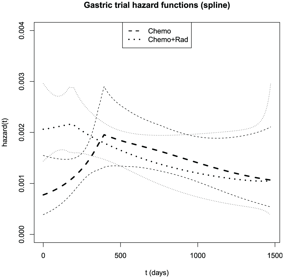
Bayesian model-averaged spline estimates of the gastric cancer trial hazard functions with pointwise standard error bars (
Example: head-and-neck cancer
Efron analyzed data from a randomized trial comparing radiation therapy alone to chemotherapy plus radiation in head-and-neck cancer.
9
Of 96 patients, 73 experienced events. Cox analysis gives a hazard ratio (favoring chemoradiotherapy) of 0.58, with 95% confidence interval (0.35, 0.91) and logrank
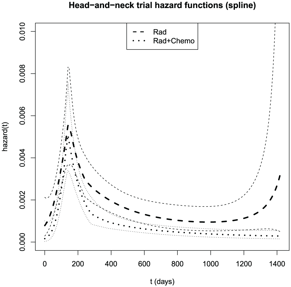
Bayesian model-averaged spline estimates of the head-and-neck cancer trial hazard functions with pointwise standard error bars (
Evaluation of the effect of coarsening
Starting with survival time t denominated in days, one can transform to weeks by taking
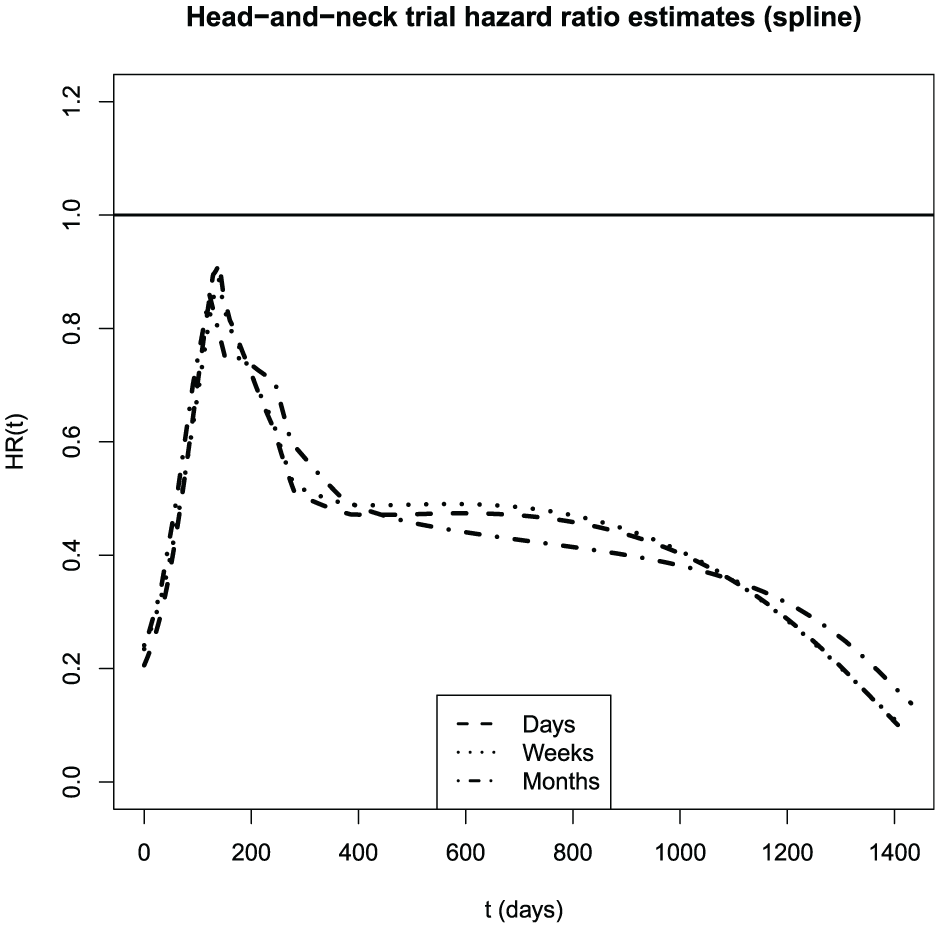
Estimates of the head-and-neck hazard ratio from the spline model by Bayesian model averaging, on three different time scales.
Discussion
Discrete versus continuous models
The models proposed here depart from common practice in treating survival as discrete. This device enables effective approximation of continuous-data models and straightforward estimation of hazards via binary regression. Most importantly, these models reflect the fact that clinical trial survival data are discrete, typically denominated in days with the possibility of zero values and ties. Thus, it is the continuous-data models that we should view as approximations, not the other way around.
My empirical findings confirm Efron’s 9 prediction that the shape of the estimated hazard function is robust to the level of discretization. Indeed, the degree of coarsening appears to have less influence on estimates than the choice of flexible modeling technique. This agrees with general observations that analysis of discrete data as though continuous is valid unless the number of distinct data values is small, perhaps fewer than 10. 32
Flexible models
Flexible-model confidence intervals were calibrated for the mean except when the underlying data were lognormal. Plausibly, this is because one can define flexible models only on the range of the data; to extrapolate beyond this range, I added an exponential tail that figured in the computation of the mean. This adjustment was evidently unsuitable for the lognormal but adequate for the others. For medians, where tail length is irrelevant, the flexible estimates were calibrated for all the parametric generating models.
In simulations, the spline model estimated all hazards well, whereas the fractional polynomial was accurate for all but the mixture hazard. This was because the fractional polynomial was not sufficiently flexible to describe the multiple modes of the mixture hazard, leading to bias. Including a third term in the fractional polynomial should address this deficiency.
Model-averaged hazard estimates inherit features of each component model. For instance, when the model space includes a linear spline with a single knot, the averaged hazard function will also have discontinuous first derivative at that knot (see Figures 2 –5 and S.7–S.9). I therefore excluded zero-order splines (step functions), which would have created discontinuities at the knots.
Extensions of the model
Various approaches to extending the flexible model are possible: increasing the number of fractional polynomial terms; 12 mixing model types in the model space; using informative priors for coefficients in the regression models; and replacing the logistic link with an alternative such as the complementary log-log.
Why estimate hazards?
Recent literature challenges the common practice of interpreting the hazard ratio as a causal parameter.3,33–37 The issue is that at any time
Its equivalence with other descriptors of survival nevertheless suggests a role for the hazard in applications. First, whereas survival curves look largely the same, declining from 1 to 0, hazards can take a wide range of shapes, including some that are characteristic of particular distributions. Therefore, estimating hazards can help distinguish distributions and suggest parametric forms for future analyses. Second, because the survival function is essentially an integrated version of the hazard, 38 it can smooth away some potentially informative detail. Consider that in the gastric cancer data, the survival curves cross only after 30 months, 29 whereas Figure 3 shows the hazard curves crossing around 12 months—substantially changing the interpretation. Third, the hazard function represents an instantaneous mortality rate, that is, in a sense, “upstream” of the survival curve and density. Thus, it is natural to conceptualize an intervention as operating at each time t to reduce the instantaneous risk, thereby increasing future survival. This idea is implicit in the ubiquitous practice of describing clinical trial treatment effects with hazard ratios. 2 Yet despite the popularity of such analyses, it continues to be rare to see graphs of estimated hazards in clinical trial practice. 38
Proportional hazards tests
Tests of the null hypothesis of proportional hazards31,39 have limited power when the departure from proportionality is modest, the sample size is small, or censoring is abundant40,41—conditions that hold in many clinical trials. It is therefore informative to inspect hazard function graphs and compare them in light of estimated error bounds.
Consider our examples: In the gastric cancer trial, the Grambsch-Therneau test is significant, and the hazard plots (Figures 3 and S.8) demonstrate marked departure from proportionality. In REMATCH, a larger trial, there was an expectation of excess early hazard reflecting perioperative mortality in the device arm. Although Grambsch-Therneau is not significant, inspection of the hazard curves (Figures 2 and S.7) reveals nonproportionality in the anticipated direction. Averaging these varying hazard ratios—some above 1.0 and others below 0.4—obscures important differences in the mortality distributions.
Conclusion
Given the hazard function’s central role in survival modeling, I recommend its estimation as a routine element of clinical trial practice.
Supplemental Material
sj-pdf-1-ctj-10.1177_17407745261439661 – Supplemental material for Estimating clinical trial hazard functions
Supplemental material, sj-pdf-1-ctj-10.1177_17407745261439661 for Estimating clinical trial hazard functions by Daniel F Heitjan in Clinical Trials
Footnotes
Acknowledgements
I thank the deputy editor, associate editor, and a referee for helpful comments.
Funding
The author disclosed receipt of the following financial support for the research, authorship, and/or publication of this article: This work was supported by grant 2208892 from the US National Science Foundation and grant ME-2012C2-22793-IC from the Patient-Centered Outcomes Research Institute.
Declaration of conflicting interests
The author declared no potential conflicts of interest with respect to the research, authorship, and/or publication of this article.
Data Availability Statement
Data and code are available in the Supplement.
Supplemental material
Supplemental material for this article is available online.
References
Supplementary Material
Please find the following supplemental material available below.
For Open Access articles published under a Creative Commons License, all supplemental material carries the same license as the article it is associated with.
For non-Open Access articles published, all supplemental material carries a non-exclusive license, and permission requests for re-use of supplemental material or any part of supplemental material shall be sent directly to the copyright owner as specified in the copyright notice associated with the article.