Estimands in clinical trials of complex disease processes

Abstract

Clinical trials with random assignment of treatment provide evidence about causal effects of an experimental treatment compared to standard care. However, when disease processes involve multiple types of possibly semi-competing events, specification of target estimands and causal inferences can be challenging. Intercurrent events such as study withdrawal, the introduction of rescue medication, and death further complicate matters. There has been much discussion about these issues in recent years, but guidance remains ambiguous. Some recommended approaches are formulated in terms of hypothetical settings that have little bearing in the real world. We discuss issues in formulating estimands, beginning with intercurrent events in the context of a linear model and then move on to more complex disease history processes amenable to multistate modeling. We elucidate the meaning of estimands implicit in some recommended approaches for dealing with intercurrent events and highlight the disconnect between estimands formulated in terms of potential outcomes and the real world.

Introduction

Clinical trials are typically designed to test intervention effects on population-level marginal features such as means or proportions, but even such a seemingly simple objective can be challenging when intercurrent events arise. In such settings, it is important to understand the meaning of potential target estimands and interpret findings accordingly. ¹ The E9 Addendum on this matter from the International Conference on Harmonization for Pharmaceutical Research ² spawned a great deal of subsequent developments in the biopharmaceutical and biostatistics literature. ³

Our aims are to outline principles for the specification of estimands for clinical trials, to point out that with some types of intercurrent events, seemingly simple marginal features may not be interpretable or relevant for patient care, and to promote continued use of the intention-to-treat principle. When disease processes are complex due to the presence of multiple events and competing risks, we point out that utility-based analyses can aid in synthesizing evidence of treatment effects. While the specification of utilities can be a challenge, our position is that they are invariably implicitly at play when readers form their own gestalt about the merit of a new treatment for a complex disease. Specification of utilities can make this process transparent and aid in decision making.

Many authors discuss causal effects of treatment in terms of potential outcomes. ⁴ In settings involving complex and dynamic disease processes, the notion that each individual has predefined paths under each possible treatment is unappealing in our view, particularly when intercurrent events may occur. Like others,^5,6 we therefore avoid the use of counterfactuals and instead stress specification of estimands that are based solely on observable aspects of a disease process. Cox ⁷ gives a wide ranging discussion of causality that stresses the importance of different points of view; see also Cox and Wermuth. ⁸

The remainder of the article is organized as follows. In Joint models for response, marker and intercurrent events, we introduce linear models involving a continuous response and a marker covariate measured repeatedly over time, and consider settings where an intercurrent event may arise. This simple framework enables clear discussion about the implications of different analysis strategies for dealing with intercurrent events. In Complex life history processes and multistate models, we discuss more complex disease processes involving multiple types of events which are amenable to multistate modeling. We consider the specification of estimands in this setting, both in the absence of intercurrent events and through the use of expanded models when intercurrent events may arise. In The utility of utilities, the appeal of incorporating utilities into multistate analyses is highlighted as a method of synthesizing evidence of treatment effects over different events. Concluding remarks are made in the Discussion.

Joint models for response, marker, and intercurrent events

A model formulation illustrating basic principles

Disease processes evolve over time. Before considering more complex situations, we discuss a simple setting involving a scalar response $Y$ and a biomarker $W$ measured at a baseline assessment time $s_0=0$ and two follow-up times $s_1,s_2$ . For a given subject, let $Z_j=(Y_j,W_j)\prime$ where $Y_j$ and $W_j$ denote the outcome and biomarker values at the assessment time $s_j$ for $j=0,1$ and $2$ . The history of the joint outcome-marker process up to the $j$ th follow-up time is ${\mathcal{Z}}_j=\{Z_0,\dots ,Z_j\}$ , $j=0,1,2$ . Let $X$ be a treatment indicator assigned by randomization at time $s_0$ , where $X=1$ and $0$ represent the experimental and control treatment, respectively; randomization ensures that $Z_0$ is independent of $X$ , which we write as $Z_0\perp X$ . A common target estimand in this setting is

$${\theta }_1=E(Y_2|X=1)-E(Y_2|X=0).$$

(1)

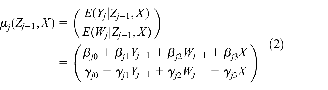
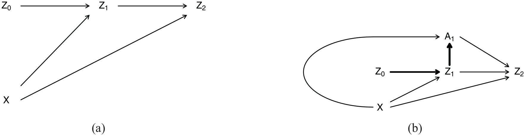
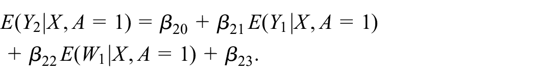
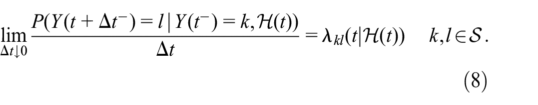
The directed acyclic graph (DAG) in Figure 1(a) shows the relationships between variables where $Z_2$ is conditionally independent of $Z_0$ given $Z_1$ and $X$ ; this is denoted by $Z_2\perp Z_0|Z_1,X$ . To facilitate illustrative calculations, we consider linear models where $Z_0~N_2({\mu }_0,{\Sigma }_0)$ with ${\mu }_0=(0,0)\prime$ , ${\Sigma }_0=\mathrm{cov}(Z_0)$ and $N_2(·)$ denotes a bivariate normal distribution. Under this first-order dependence model, $Z_j|{\mathcal{Z}}_{j-1},X~N_2({\mu }_j(Z_{j-1},X),{\Sigma }_j)$ , and we suppose that

$$\begin{array}{c}{\mu }_j(Z_{j-1},X)=\left(\begin{array}{c}E(Y_j|Z_{j-1},X)\hfill \\ E(W_j|Z_{j-1},X)\hfill \end{array}\right)\hfill \\ =\left(\begin{array}{c}{\beta }_{j0}+{\beta }_{j1}{Y}_{j-1}+{\beta }_{j2}{W}_{j-1}+{\beta }_{j3}X\hfill \\ {\gamma }_{j0}+{\gamma }_{j1}{Y}_{j-1}+{\gamma }_{j2}{W}_{j-1}+{\gamma }_{j3}X\hfill \end{array}\right)\hfill \end{array}$$

(2)

and ${\Sigma }_j=\mathrm{cov}(Z_j|{\mathcal{Z}}_{j-1},X)$ , $j=1,2$ . In this framework, the target estimand (1) is expressed as

$$E(Y_2|X=1)-E(Y_2|X=0)={\beta }_{21}{\beta }_{13}+{\beta }_{22}{\gamma }_{13}+{\beta }_{23}$$

(3)

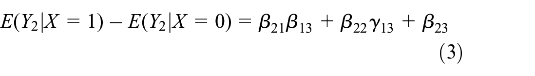
where ${\beta }_{21}{\beta }_{13}+{\beta }_{22}{\gamma }_{13}$ is the indirect effect of $X$ on $Y_2$ mediated through $Z_1=(Y_1,W_1)\prime$ , and ${\beta }_{23}$ is the direct effect of $X$ on $Y_2$ . ⁹ We call ${\theta }_1$ in (1) a marginal effect since it does not involve conditioning on any baseline or intermediate variables except for $X$ . If there are no dropouts or other intercurrent events, ${\theta }_1$ is estimable as the difference in mean responses for the treatment and control groups. A more detailed secondary analysis would be to examine indirect and direct treatment effects through the model (2).

Figure 1.

Directed acyclic graphs showing the relation between $X,Z_0,Z_1$ , and $Z_2$ without and with an intercurrent event $A_1$ : (a) a simple DAG relating $Z_j=(Y_j,W_j)$ , $j=0,1,2$ , and $X$ and (b) an expanded DAG incorporating an intercurrent event $A_1$ with $A_1\perp Z_0|Z_1,X$ .

This simple model is an idealization, but represents a broad range of trials involving repeated measurement of specific markers along with clinical outcomes. For example, in trials of respiratory disease, inflammation markers may be collected at follow-up with responses based on an outcome such as forced expiratory volume. In rheumatology trials, one may aim to assess treatment effects on disease burden or quality of life, but record erythrocyte sedimentation rate at follow-up assessments as well. Likewise in a trial comparing intensive to conventional insulin therapy on complications from Type 1 diabetes, ¹⁰ the degree of diabetic retinopathy was of primary interest but accompanied by measurement of HbA1C (glycosylated hemoglobin, a measure of blood glucose control) at quarterly assessments. We next turn to complications arising from intercurrent events in such settings.

Complications arising with intercurrent events

We now consider a setting in which an intercurrent event can arise and be realized at time $j=1$ , with its occurrence and non-occurrence indicated by $A_1=1$ and $0$ , respectively. We use the same symbol $A_1$ to denote three distinct settings to highlight that they are often viewed as similar problems, but our point is that while they can be described using similar notation, they are in fact quite different problems and should be handled differently. We explain this in what follows.

For simplicity, we assume $A_1\perp Z_0|Z_1,X$ but $Z_1=(Y_1,W_1)$ may influence its occurrence with

$$P(A=1|Z_1,X)=\mathrm{expit}({\alpha }_0+{\alpha }_1{Y}_1+{\alpha }_2{W}_1+{\alpha }_{3}X).$$

(4)

The expanded DAG in Figure 1(b) shows the relations between variables in this setting.

Approaches for handling intercurrent events have been actively discussed by regulators and biostatisticians. The ICH-E9 addendum lists five approaches targeting different estimands: (1) the “treatment policy” strategy under which outcomes are attributed to the treatments individuals are assigned to; (2) the “hypothetical” strategy in which estimands are targeted to correspond to a different scenario than the one of the trial; (3) the use of composite outcomes; (4) the “while on treatment” approach; and (5) methods based on principal stratification. ² Intercurrent events vary by their nature, and different strategies may be more or less reasonable depending on the type of event. We consider three types of intercurrent events: (1) ones that prevent observation of the response of interest (e.g. study withdrawal); (2) ones that change the interpretation of the response of interest (e.g. introduction of rescue therapy); and (3) ones that preclude observation of the response of interest (e.g. death). We illustrate them in turn.

Intercurrent event related to study withdrawal

Suppose that $A_1=1$ indicates that an individual completed the trial, so that $Y_2,W_2$ are observed; $A_1=0$ indicates withdrawal before time $j=2$ . Based on equation (2), the means among individuals who completed the trial are

$$\begin{array}{c}E(Y_2|X,A=1)={\beta }_{20}+{\beta }_{21}E(Y_1|X,A=1)\hfill \\ +{\beta }_{22}E(W_1|X,A=1)+{\beta }_{23}.\hfill \end{array}$$

This implies the estimand $E(Y_2|X=1,A=1)-E(Y_2|X=0,A=1)$ given by

$${\beta }_{21}[{\mu }_{1A}(1)-{\mu }_{1A}(0)]+{\beta }_{22}[{\mu }_{2A}(1)-{\mu }_{2A}(0)]+{\beta }_{23}$$

(5)

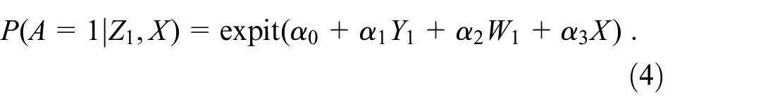
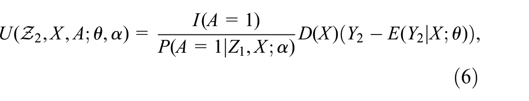
where ${\mu }_{1A}(X)=E(Y_1|X,A=1)$ and ${\mu }_{2A}(X)=E(W_1|X,A=1)$ . Note that if ${\alpha }_1={\alpha }_2=0$ in equation (4) then $Z_2$ is missing at random (MAR). ¹¹ Then ${\mu }_{1A}(1)-{\mu }_{1A}(0)={\beta }_{13}$ , ${\mu }_{2A}(1)-{\mu }_{2A}(0)={\gamma }_{13}$ and equation (5) reduces to equation (3), which can then be estimated by the difference in mean responses in the treatment and control groups among persons completing the trial. When ${\alpha }_1$ or ${\alpha }_2$ are not zero, $A_1$ is not independent of $Z_1$ given $X$ , and $Z_2$ is not MAR. Conditioning on $A_1=1$ creates a selection bias, ¹² which is referred to as a “collider bias” when viewing the phenomenon through the DAG of Figure 1(b), since the arrows from $Z_0$ and $X$ and collide at $A_1$ . ¹³ In that case multiple imputation or weighting can produce pseudo-samples representative of a target population in which $A_1\perp (Z_1,X)$ . To fit $E(Y_2|X)={\theta }_0+{\theta }_{1}X$ , where ${\theta }_1$ is (3), an inverse probability weighted estimating function is

$$\begin{array}{c}U({\mathcal{Z}}_2,X,A;\theta ,\alpha )=\frac{I(A=1)}{P(A=1|Z_1,X;\alpha )}D(X)(Y_2-E(Y_2|X;\theta )),\hfill \end{array}$$

(6)

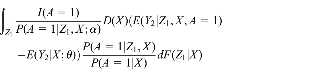
where $D(X)=(1,X)\prime$ . To show that equation (6) is an unbiased estimating function, we first take the expectation with respect to $Y_2|Z_1,X,A=1$ and then with respect to $Z_1|X,A=1$ to obtain

$$\begin{array}{c}{\int }_{Z_1}\frac{I(A=1)}{P(A=1|Z_1,X;\alpha )}D(X)(E(Y_2|Z_1,X,A=1)\hfill \\ -E(Y_2|X;\theta ))\frac{P(A=1|Z_1,X)}{P(A=1|X)}\mathit{dF}(Z_1|X)\hfill \end{array}$$

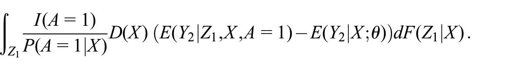
where $\mathit{dF}(Z_1|X,A=1)=P(A=1|Z_1,X)\mathit{dF}(Z_1|X)/P(A=1|X)$ . Under the positivity condition $P(A=1|Z_1,X)>0$ , cancelation of $P(A=1|Z_1,X;\alpha )$ means the second expectation effectively becomes one with respect to $Z_1|X$ giving

$$\begin{array}{c}{\int }_{Z_1}\frac{I(A=1)}{P(A=1|X)}D(X)(E(Y_2|Z_1,X,A=1)-E(Y_2|X;\theta ))\mathit{dF}(Z_1|X).\hfill \end{array}$$

For this to have expectation zero, we require $E\{E(Y_2|Z_1,X,A=1)|X\}=E(Y_2|X;\theta )$ which in turn requires $E(Y_2|Z_1,X,A=1)=E(Y_2|Z_1,X,A=0)$ . Thus, reweighting the available data in equation (6) creates a pseudo-sample representative of the target population from which the full sample is drawn. This adjustment for selective attrition through weighting only addresses one aspect of loss to follow-up, however, corresponding to condition (4a) of Lawless and Cook. ¹⁴ The more subtle condition is $E(Y_2|Z_1,X,A=1)=E(Y_2|Z_1,X,A=0)$ , corresponding to (4b) of Lawless and Cook; ¹⁴ this states that the conditional mean response of those who dropped out is the same as those who remained in the study. This may be true, but is only possible to check through tracing studies.

Intercurrent event is introduction of rescue treatment

Now consider the setting where the $A_1$ indicates the introduction of rescue medication. Here, we suppose the data generating model is

$$E(Y_2|Z_1,X,A)={\beta }_{20}+{\beta }_{21}{Y}_1+{\beta }_{22}{W}_1+{\beta }_{23}X+{\beta }_{24}A$$

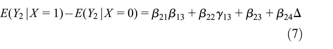
where ${\beta }_{24}$ reflects the additional effect of the rescue therapy. The need to expand the model to incorporate an effect of the rescue therapy makes this a fundamentally different issue than one of study withdrawal. If the goal is to examine the “total” average causal effect of $X$ on $Y_2$ , since $Z_0\perp X$ and $E(Y_2|X)=E_{Z_1,A}\{E(Y_2|Z_1,X,A)|X\}$ we have

$$\begin{array}{c}E(Y_2|X=1)-E(Y_2|X=0)={\beta }_{21}{\beta }_{13}+{\beta }_{22}{\gamma }_{13}+{\beta }_{23}+{\beta }_{24}\mathrm{\Delta }\hfill \end{array}$$

(7)

where

$$\begin{array}{c}\mathrm{\Delta }=E_{Z_1}\{P(A=1|Z_1,X=1)|X=1\}\hfill \\ -E_{Z_1}\{P(A=1|Z_1,X=0)|X=0\}.\hfill \end{array}$$

Note that even if $A_1\perp X|Z_1$ , there is an effect of $A_1$ on the marginal causal effect $\left({\beta }_{24}\mathrm{\Delta }\right)$ , unless (1) $A_1\perp Z_1|X$ (i.e. if “rescue therapy” is administered independently of $Z_1$ given $X$ ) or (2) $Z_1\perp X$ (i.e. if there is no effect of treatment on $Z_1$ ); both (1) and (2) give $\mathrm{\Delta }=0$ but neither condition is usually satisfied in practice. An intention-to-treat analysis which does not incorporate $A_1$ into the model is aligned with the treatment policy framework and is preferred in such settings; ¹⁵ the corresponding estimand is (7) rather than (3). See also Cox ⁷ for related discussion.

Censoring (i.e. removing) individuals from the analysis after the introduction of rescue treatment is often proposed, with inverse weighting used in an attempt to estimate the average causal effect in the spirit of the example of withdrawal. This is problematic—use of weights such as those in equation (6) creates a pseudo-sample in which $A_1\perp Z_1|X$ , but this is not aligned with the real world where rescue treatments are prescribed based on patient need (here reflected by $Z_1$ ). Second, we note that the more subtle condition implicit when inverse weighting, that $E(Y_2|Z_1,X,A=1)=E(Y_2|Z_1,X,A=0)$ , is patently violated if the rescue treatment has any effect. Introduction of rescue treatment is therefore a fundamentally different problem than study withdrawal.

Intercurrent event is death

While “intercurrent” seems an inappropriate term for death, it is often considered an intercurrent event since it may preclude observation of the response at a planned assessment time. For illustration, we suppose $A_1$ indicates survival to $j=2$ and an analyst plans to compare the mean response between treatment arms among individuals who survived. We stress that this situation is fundamentally different from either of the previous two settings. Loss to follow-up is an inconvenience and one can reasonably aim to mitigate bias due to selective attrition, and in the case of rescue treatment, one may still observe $Y_2$ . Death, however, is an integral part of the response process and survivors to time $j=2$ typically do not produce a random sample of persons randomized to either $X=1$ or $X=0$ . Trying to use weights in the same spirit as discussed earlier to render $A_1\perp Z_1|X$ does not align with the biological process in which $Z_1$ is associated with survival status. In addition, the response $Y_2$ does not exist among individuals who died so the condition $E(Y_2|Z_1,X,A=1)=E(Y_2|Z_1,X,A=0)$ is meaningless.

The survivor average causal effect ⁴ defines an effect based on potential outcomes $Y_2^X$ , $X=0,1$ among individuals who would survive under either treatment. As stated earlier, we avoid potential outcomes and note that these individuals are not identifiable. An estimand based on the difference in potential outcomes, $Y_2^1-Y_2^0$ , among persons surviving to $j=2$ under both treatments does not correspond to a real biological process.

Causal inference regarding treatment effects on measures of disease activity or progression is challenging when mortality rates are non-negligible. In The utility of utilities, we point out that utility-based analyses offer a useful framework for integrating disease-related and survival responses, but we first discuss issues involved in multistate processes.

Complex life history processes and multistate models

In phase III clinical trials involving cancer, cardiovascular disease and many other conditions individuals are at risk of multiple possibly competing events. Multistate models with a state space $s=\{0,1,\dots \}$ offer a powerful framework for studying such processes. We assume all subjects begin a trial in state $0$ , and that states $1,2,\dots$ represent different types of events that an individual may experience during the trial. ¹⁶ With cardiovascular disease, for example, states $1,2,3$ might represent stroke, myocardial infarction, and death, respectively. ¹⁷ Intercurrent events can also be represented by states. ¹⁸ In this setting, event occurrence and time-varying covariates are assumed to evolve in continuous time.

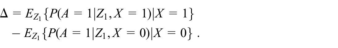
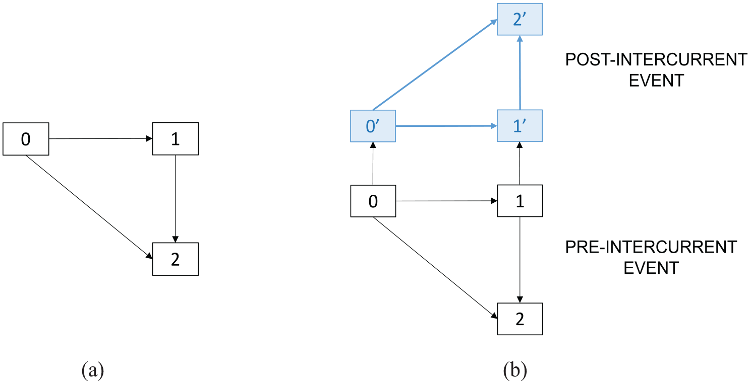
The illness-death process with state space $\mathcal{S}=\{0,1,2\}$ depicted in Figure 2(a) is a canonical multistate model that incorporates a non-fatal event (state 1) and death (state 2). In a randomized trial, state 1 often represents an event such as disease progression or recurrence. We consider it for the discussion that follows. Let $Y(t)$ represent the state occupied at time $t$ from randomization; $\{Y(s),0<s\}$ is the multistate process, with $Y(0)=0$ . We let $\{W(s),0<s\}$ represent an associated marker process; together these give a process history up to time $t$ which we denote by $\mathcal{H}(t)=\{Y(s),W(s),0<s<t,X\}$ . For convenience, we include the assigned treatment $X$ for a subject in their process history. Such multistate processes are specified in terms of intensity functions that represent the probability of specific events (i.e. changes of state) at time $t$ , conditional on the prior process history. Formally, the intensity function for a transition from state $k$ to state $l$ is defined as^16,19

$$\underset{\mathrm{\Delta }t\downarrow 0}{lim}\frac{P(Y(t+\mathrm{\Delta }{t}^{-})=l|Y(t^{-})=k,\mathcal{H}(t))}{\mathrm{\Delta }t}={\lambda }_{\mathrm{kl}}(t|\mathcal{H}(t))k,l\in \mathcal{S}.$$

(8)

Figure 2.

(a) An illness-death process and (b) a joint model for an illness-death and intercurrent event process.

Disease processes are dynamic, with both time (e.g. age, disease duration, or time on study) and the disease history playing a central role in modeling the course of disease. Intensity functions are defined in terms of these features and they provide insights into disease dynamics. Time plays a central role in connection with causal effects, and some schools of causality are focused on intensities. Intensity-based analyses are central to study of what ²⁰ refer to as “dynamic causality.” At the same time, intensities do not allow randomization to be used as a basis for inferring causal effects. It is well known that conditioning on the process history can induce a “collider bias”^21–23 if important variables are omitted. This point was illustrated in Complications arising with intercurrent events in the context of a complete case analysis when data are missing at random—there conditioning on $A_1=1$ induced confounding and yields biased estimates of the target causal effect. Furthermore, unmeasured confounders that by virtue of randomization are independent of assigned treatment $X$ at the start of the trial will not generally be independent of $X$ among subjects in some particular state at time $t>0$ . This invalidates simple comparisons of intensities for the two treatment groups. Since it is desirable to take advantage of randomization to make robust treatment comparisons (i.e. to define estimands that can be robustly estimated and assigned a causal interpretation), primary planning, testing and estimation of effects, and regulatory decision making are typically based on marginal process features such as the occurrence of a specific event by a certain time.^18,19,24

This highlights a paradox that understanding of causal mechanisms is best done through intensity-based models and related measures characterizing disease processes, but primary estimation and testing in randomized trials is based on causal effects related to simple marginal estimands. Indeed, clinical trials are not primarily designed to enhance understanding of causal mechanisms, but rather to robustly demonstrate marginal (population-level) causal effects. We stress, however, the important role of intensity-based analyses to understand reasons for marginal causal effects and to study intercurrent events and their effect on the disease process under study.^18,25 Analogously to the case of the linear model in Joint models for response, marker, and intercurrent events, conditional intensity-based analyses can also yield insights on causal mechanisms through mediation analyses.^20,26

There are several marginal features that may be of interest for the process in Figure 2(a), including (a) the probability of entry to state 1 by a given time, (b) the probability of death (entry to state 2) by a given time, (c) the restricted mean lifetime over some time interval $(0,\tau ]$ , and (d) the probability of remaining event-free (i.e. in state 0) up to a given time. Cumulative incidence functions and survivor functions (or more generally state occupancy probabilities $P(Y(t)=k|Y(0)=0)$ ) provide estimands of such quantities and we discuss them next.

If $T_k$ denotes the entry time to state $k$ , $k=1,2$ in the illness-death process, the cumulative incidence function for entry to state 1 is $F_1(t)=P(T_1<t|Y(0)=0)$ . General transformation models are widely used: they are defined by specifying a link function $g(·)$ and setting

$$g(F_1(t))={\alpha }_1(t)+{\beta }_{1}X.$$

(9)

The model using the complementary log-log link $g(u)=\log (-\log (1-u))$ is often called the Fine-Gray model, though it was first proposed in connection with the sub-hazard function for $T_1$ . Similar models apply when there are two or more states besides state $1$ that may be entered from state $0$ . Estimation of the treatment effect ${\beta }_1$ can be approached in different ways. ²⁵ Some other marginal features are based on state occupancy probabilities $P(Y(t)=k)$ ; for example, option (d) above (often called event-free survival) is given by $P(Y(t)=0)$ . Occupancy probabilities can be estimated robustly using the nonparametric Aalen-Johansen estimate of the transition probability matrix, ²⁷ giving robust estimates of estimands such as $P(Y(t)=0|X=1)-P(Y(t)=0|X=0)$ .

It should be noted that marginal features such as $F_1(t|X)$ or $P(Y(t)=k|X)$ are typically complex functions of the process intensities, and the effect of treatment on the intensities. Secondary intensity-based analysis is needed to understand effects based on marginal features, along with checks of the models on which they are based. In general, the more complex the disease process, the more difficult it is to specify a single one-dimensional estimand on which to base treatment comparisons and tests. In the next section, we discuss the use of utility functions that combine different aspects of a process.

When intercurrent events can arise, the specification of estimands is more challenging. Figure 2(b) depicts a joint model for an illness-death process and a non-fatal intercurrent event. Here 0 represents the state of being alive and free of the non-fatal clinical event of interest, as well as the intercurrent event, state 1 is entered when an individual experiences the non-fatal clinical event but has not had the intercurrent event, and state 2 is entered by individuals who die intercurrent-event free. States $0\prime$ , $1\prime$ , and $2\prime$ are the corresponding states following an intercurrent event. ¹⁴ Give a discussion of independent right-censoring which is important if the intercurrent event is study withdrawal. Inverse probability of censoring weights can mitigate the effects of selective withdrawals, but when viewing the process as in Figure 2(b), there is an additional implicit assumption that the $k\prime \to l\prime$ transition intensities post-withdrawal equal their $k\to l$ counterparts for persons remaining in the trial. This assumption is not checkable unless individuals are followed after they leave the trial.

When the intercurrent event is the introduction of rescue therapy, some ²⁸ suggest censoring at that time and using inverse probability weights to adjust for factors related to the administration of rescue therapy. As discussed in Joint models for event, marker, and intercurrent events, censoring at the time of rescue therapy and use of inverse probability of censoring weighting does not target an interpretable estimand in the real world. Information is typically available regarding $k\prime \to l\prime$ transitions post rescue therapy and thus one can model the full process in Figure 2(b). This enables estimation of features under the treatment policy or intention-to-treat framework discussed in Complications arising with intercurrent events. The treatment policy estimand (perhaps based on $P(\mathcal{Z}(t)\in \{2,2\prime \}|\mathcal{Z}(0)=0,X)$ ) is a sensible target; this addresses the fact that treatments may need to be modified in patient care and so reflects clinical practice. However, trialists should be sure to recruit sites and protocolize standard of care to ensure that this estimand has the desired interpretation.

The utility of utilities

Synthesis of evidence across different features of a process can be formalized through the specification of fixed or time-varying utilities associated with different life history paths or states.^29,30 We address this briefly here.

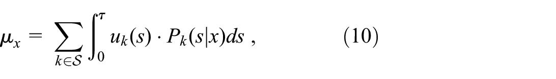
Let $u_k(s)$ be the utility of being in state $k$ at time $s\ge 0$ with $0\le u_k(s)\le 1$ for $k\in \mathcal{S}$ . The restricted mean cumulative utility over a specified time interval $(0,\tau ]$ , given $X=x$ , is then

$${\mu }_x=\sum _{k\in \mathcal{S}}{\int }_0^{\tau }{u}_k(s)·P_k(s|x)\mathit{ds},$$

(10)

where $P_k(s|x)=P(Y(s)=k|Y(0)=0,X=x)$ . Model-free estimands such as ${\mu }_1-{\mu }_0$ or ${\mu }_1/{\mu }_0$ can then be defined. They can be estimated robustly by using nonparametric Aalen–Johansen estimates ²⁷ for state occupancy probabilities. A special case of this is restricted mean survival time ³¹ under a $0\to 1$ survival process which is given by $u_0(s)=1$ and $u_1(s)=0$ for all $s>0$ . Utility functions are also aligned with quality adjusted life years analysis routinely employed in cancer clinical trials where trade-offs are necessary between treatment toxicity and effectiveness.^32,33

This approach also offers a way of incorporating information on intercurrent events in the assessment of randomized interventions. For example, with fixed state-dependent utilities for the illness-death process of Figure 2(a), suppose state 0 is assigned a utility of 1 and state 1, representing disease progression, say, has a utility of 0.8. If state 2 represents death, then it would have a utility of 0, giving $u_0=1,u_1=0.8,u_2=0$ . If ${\hat{P}}_k(s|x)$ is the Aalen–Johansen estimate from the group with $X=x$ , ${\hat{\mu }}_x=\sum _{k\in S}{\int }_0^{\tau }{u}_k{\hat{P}}_k(s|x)\mathit{ds}$ where $S=\{0,1,2\}$ . If the intercurrent event is the introduction of rescue therapy, for the purposes of evaluating the effect of the randomized treatment it may be desirable to discount the utility of some subsequent health states and so in the joint model of Figure 2(b) one might set $u_{0\prime }=0.9$ , $u_{1\prime }=0.7$ , with $u_{2\prime }=0$ . In this case, $S_I=\{0,1,2,0\prime ,1\prime ,2\prime \}$ is the expanded state space incorporating the intercurrent event and we obtain ${\tilde{\mu }}_x=\sum _{k\in S_I}{\int }_0^{\tau }{u}_k{\tilde{P}}_k(s|x)\mathit{ds}$ where ${\tilde{P}}_k(s|x)$ is the Aalen–Johansen estimate of the transition probability matrix for Figure 2(b). Tertiary analyses can be carried out involving alternative sets of utilities for a sensitivity analysis when values are hard to set by consensus or if there is interest in assessing the merit of treatment from different perspectives.

Discussion

Many of the issues discussed here are causal in nature but, like others, ⁵ we have purposefully avoided the use of potential outcomes. While conceptualization of potential outcomes can sometimes be useful, in settings involving complex dynamic processes, the notion of pre-defined paths under each treatment assignment is unappealing, particularly when intercurrent events can arise. More importantly, as we argued in the case of the survivor average causal effect, one can be lead to defining estimands which do not represent a well-defined and observable population of patients.

We support the use of treatment effects based on observable marginal features of a process, along with secondary intensity-based analysis to provide an understanding of a marginal effect. We also support the treatment policy (intention to treat) strategy for dealing with intercurrent events whenever possible. As others have,^7,34 we emphasize that a thorough understanding of causation involves several points of view and, especially for the study of dynamic processes, explicit consideration of the effects of time. For complex processes, it is not always desirable to define a single marginal feature for the planning and primary analysis of a trial. It may be of interest to incorporate information on both $\{Y(s),0<s\}$ and $\{W(s),0<s\}$ , for example. In that case, utilities can play a helpful role for synthesizing data and making transparent treatment comparisons. Methods for setting utilities have been developed in some contexts (e.g. the health economics literature), and there are good arguments for their broader application. ³⁵ Other approaches that have been suggested are based on composite outcomes or multivariate outcomes. The former implicitly gives equal weight to different events; for example in a cardiovascular trial, an outcome may incorporate non-fatal and fatal events into a single event count. ³⁶ This is less appealing than assigning utilities to different types of events. Win ratio methods rank outcomes (i.e. process histories) and then make pairwise comparisons of observed outcomes for treatment and control subjects. ³⁷ This often ignores the relative severities of different events or states. Bühler et al. ¹⁸ show that in the illness-death model, a win ratio can be related to a utility-based approach.