
Abstract
The win ratio has been increasingly used in trials with hierarchical composite endpoints. While the outcomes involved and the rule for their comparisons vary with the application, there is invariably little attention to the estimand of the resulting statistic, causing difficulties in interpretation and cross-trial comparison. We make the case for articulating the estimand as a first step to win ratio analysis and establish that the root cause for its elusiveness is its intrinsic dependency on the time frame of comparison, which, if left unspecified, is set haphazardly by trial-specific censoring. From the statistical literature, we summarize two general approaches to overcome this uncertainty—a nonparametric one that pre-specifies the time frame for all comparisons, and a semiparametric one that posits a constant win ratio across all times—each with publicly available software and real examples. Finally, we discuss unsolved challenges, such as estimand construction and inference in the presence of intercurrent events.
Introduction
It is widely accepted that the traditional time-to-first-event analysis of a composite endpoint is less than ideal.1,2 The first event mixes patient death with lesser events, such as hospitalization, and ignores whatever happens to the patient afterward (in case of a nonfatal first event). Yet it is not until in the recent decade that some other method gained enough traction to become a viable alternative.
Win ratio and hierarchical endpoints
The new method is called the win ratio, first proposed in the work by Pocock et al. 3 in 2012 in the European Heart Journal. It compares each pair of treated and untreated patients through a hierarchy of endpoints, for example, death > hospitalization > 6-min walk test (6MWT), 4 with a lower component considered only if the prioritized ones are inconclusive. This allows more data to be used, and, more importantly, it prioritizes patient survival over nonfatal clinical events and, in turn, possibly other “softer” endpoints, such as quality-of-life measures and biomarkers. As a summary of treatment effect, the proportion of “wins” by the treatment is divided by that of their “losses” against the control. Close relatives5,6 of the win ratio include the proportion in favor of treatment (or net benefit), 7 which uses the difference rather than ratio, and the win odds,8–10 which gives the numerator and denominator each half of the “ties.”
This type of approach, and the idea of a hierarchical composite it facilitates, quickly grew in popularity.11–14 A reckoning of the online registry ClinicalTrials.gov finds a sharp rise in recent years in both the number of trials that adopt this methodology and the total number of patients involved (Figure 1). Most of the trials are cardiovascular in nature, 15 some in disease areas such as cancer and diabetes. In a high-profile case, an early variation of the win ratio (namely, Finkelstein–Schoenfeld method) 5 in the ATTR-ACT trial supported the Food and Drug Administration (FDA) approval of tafamidis in 2019 for the treatment of cardiomyopathy. 16
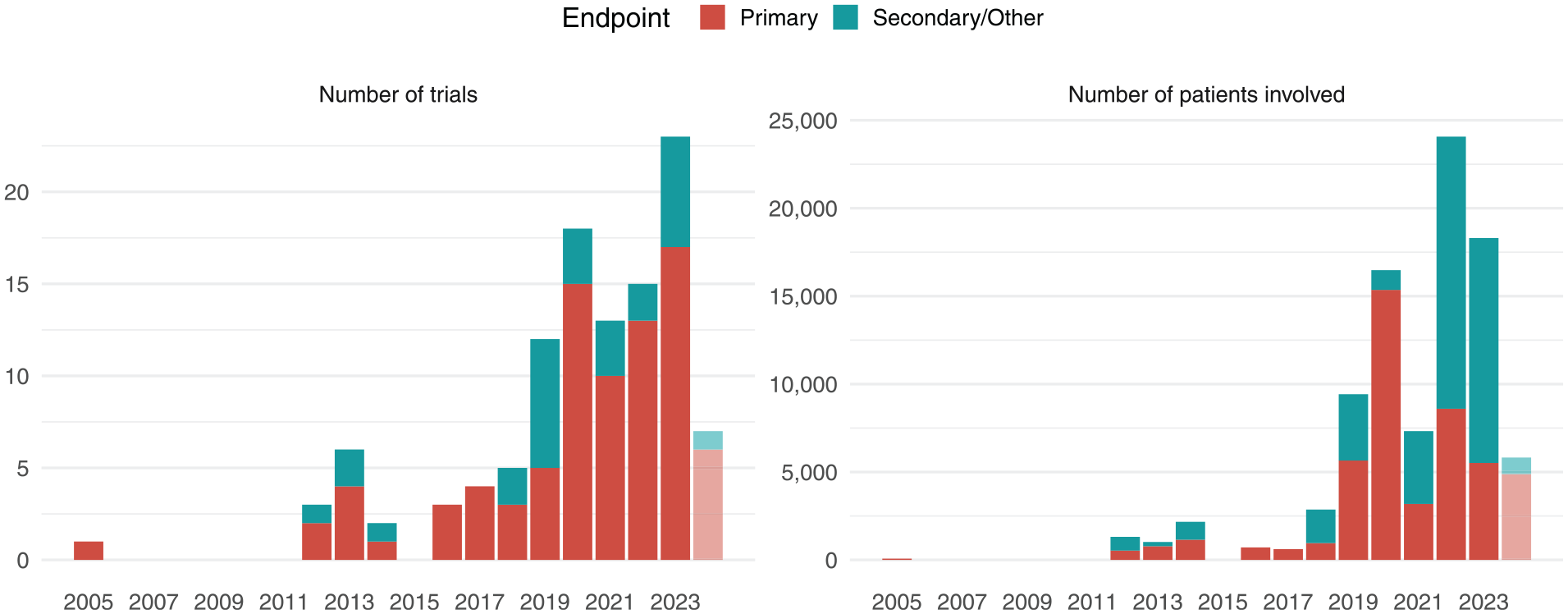
Registered trials (by start year) that specify win ratio-like approach to hierarchical composite endpoints in primary, secondary, or other analyses.
Impact of censoring on estimand
The win ratio has its downsides. A notable one is that its estimand, that is, the population-level quantity estimated by the sample-based statistic, varies with the censoring distribution. The statistical literature on this phenomenon has grown fairly rich and complete.17–21 However, some explanations in practical terms may help the applied researcher to better understand its cause and implications.
Censoring decides the time frame of comparison
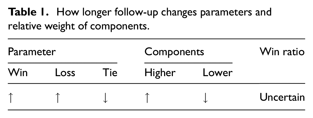
Simply put, the estimand’s dependency on censoring is caused by the fact that different time frames are used to compare patient pairs censored at different times. This creates a mixture of comparisons whose underlying time frames lack consistency. Recall that two patients censored differently are compared through their minimum follow-up time. 3 For example, consider a pair whose minimum follow-up is 1 year (e.g. one patient censored at Year 1 and the other at, say, Year 2). This means that their comparison is based on the data collected during the first year. Consider another pair in which neither patient is censored until Year 5. For them, the time frame of comparison is much longer. In this longer time, ties are less likely as there is more stuff (events) to compare on. So both the win and loss probabilities go up (regardless of the treatment effect). It also happens that win–loss is more likely to be determined by prioritized components, as they are more likely to give conclusive results and thus harder to pass (in an extreme case, if most patients die within 5 years, then hospitalization would be of no use). Figure 2 illustrates how the win–loss status, and its deciding component, changes over time. In brief, censoring sets the time frame of comparison, which systematically influences the magnitude of win–loss proportions and the relative contributions by components (Table 1). In the end, the estimand is an average of shorter-term (e.g. 1-year) versus longer-term (e.g. 5-year) comparisons weighted by the censoring distribution. 19
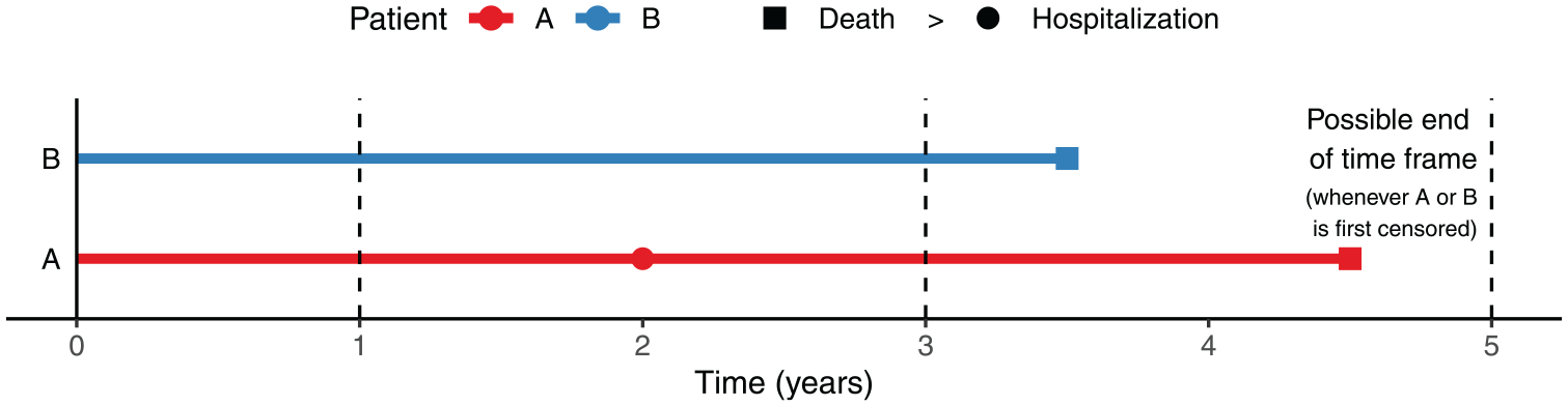
An example of win–loss outcome changing over time.
How longer follow-up changes parameters and relative weight of components.
Bias versus ambiguity in estimand
Some call this the “bias” due to censoring—that is, if you have an estimand in mind to begin with. Sometimes this is almost true. For example, every outcome measure on ClinicalTrials.gov has a “time frame” tag, supposedly specifying the period over which patient outcomes are to be collected for analysis. In that case, a natural estimand would be the (population) win ratio with all patients followed over the same period of time. However, because of staggered entry or random withdrawal, some patients may have shorter follow-up than specified. A naive calculation would bias the win–loss estimands in directions opposite to those listed in Table 1 (since follow-up is shorter than the target). Here what needs to be done is correct the bias by addressing the curtailed follow-up in the observed data (more on this later).
More often there is no clear estimand in mind. The intrinsic dependency of the measure on the time frame is ignored, and a single measure of effect size is reported as if universal in nature. To be fair, this is not completely without merit. In any case, the win ratio statistic is still a (censoring-)weighted average of the time (frame)-dependent win ratios, much like the hazard ratio statistic being one of the time-dependent hazard ratios in case of non-proportional hazards (PH). 22 Moreover, to test certain hypotheses where the treatment performs consistently better than the control over time, the win ratio does offer a valid test with desirable properties.17,20 (The analogy with the univariate case is that the log-rank statistic offers a valid test of ordered-hazards alternatives even without proportionality.) 23
Importance of estimand as a measure of effect size
More care is needed when it comes to estimation, whose aim is to quantify the treatment effect. To do so, one needs to articulate the way the effect is measured on the target population. This requires an estimand that is generalizable and not subject to change by the design and logistics of specific trials, which is not true of the win ratio, as shown in Table 1. For one thing, it is hard to compare trials lasting different lengths, let alone perform a meta-analysis thereof. Even for trials of similar durations, factors affecting the stochastic distribution of follow-up times within the trial, for example, are more patients recruited toward the beginning or the end, can move the result in ways not controlled by the investigator.
What’s more, the International Council for Harmonization of Technical Requirements for Pharmaceuticals for Human Use (ICH), an initiative to build consensus on the evaluation of medicinal products around the world, recently issued an “addendum on estimands and sensitivity analysis” to the “guideline on statistical principles for clinical trials” (ICH E9 (R1)). 24 The addendum demands clarity in the way treatment effect is measured, which it sees as one of the “central questions for drug development and licensing.” It also lists four key attributes of a meaningful estimand, namely, the treatment, target population, endpoint, and population-level summary. 25 The associated training material specifically warns that “missing data and loss-to-follow-up are irrelevant to the construction of estimands.” 26 The document has since been adopted by the FDA and European Medicines Agency (EMA), both regulatory members of the ICH, and is in the final step of implementation (Step 5).27,28
What this means for the win ratio
All this calls for attention to the estimand of the win ratio. A valid estimand should summarize the scientific variables (endpoints) without entangling censoring (though the latter must be dealt with in estimation). The question is both old and new. Old because censoring predates win ratio (no pun intended) and affects univariate and composite endpoints alike. New because win ratio involves multiple outcomes, with a pairwise-comparison routine that is complicated both arithmetically and statistically. With a bit more care, however, and some instructive comparisons with the univariate case, we can realign the win ratio toward the requisite estimand-driven framework.
Two approaches to estimand construction
Since ambiguity in the estimand is due to stochastically shifting time frames, there are two ways to pin it down. One is to fix the time frame, which can be done nonparametrically. The other is to posit a measure that stays constant over time, which requires a (at least semiparametric) temporal model.
Time restriction: a nonparametric approach
The idea of pre-specifying a time horizon to measure the outcome is hardly new. We have mentioned, for example, that each outcome measure on ClinicalTrials.gov is listed with a “time frame” attribute (e.g. 6 and 12 months, 5 years, etc.), though it is not always used to define an estimand explicitly.
Time restriction in univariate setting
For time-to-event outcomes, it is particularly helpful, even mandatory, to specify the time frame over which events are counted. In breast cancer, for example, it is common to report the 5-year survival rate (relative to the healthy population).
29
Let
Better yet, the survival rates over a time range, say from 0 to
Time-restricted win ratio
A lesson learned from the simple setting above is that the estimand should summarize the latent, structural variable uncorrupted by censoring. This feels natural and effortless if the outcome is just
The key is to envision all patients followed to the same restriction time
Start with the univariate case. The survival time up to
Hence, the treated are
The composite case is similar. For simplicity consider a two-tiered composite with a single nonfatal event (hospitalization) time
with corresponding win ratio estimand
More generally, the outcome may comprise multiple types of (possibly recurrent) events,
31
complete with biomarkers or patient-reported quality-of-life scores. Let
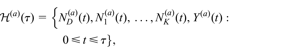
containing all event trajectories and longitudinal measurements during
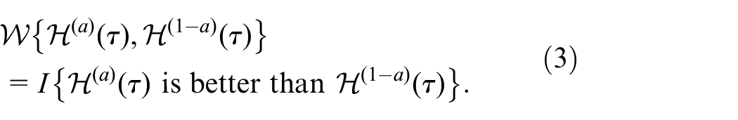
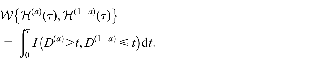
Then the
Techniques in estimation
We have seen that defining a time-restricted estimand for composite endpoints is conceptually no more complex than one for a univariate endpoint. The difficulty in estimating it, however, increases with the number of variables. This has to do with how censoring is handled.
It is true that one can specify a small
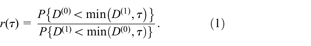
To work around it in the univariate case is relatively easy. One can express the estimand as a function of the outcome distribution, which can then be estimated in the presence of censoring by the Kaplan–Meier method. For example, we can rewrite Equation (1) by
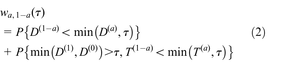
The challenge in the general case is not that a relationship between the estimand and outcome distribution fails to hold, but that the outcome distribution is harder to estimate with multiple censored components. Indeed, we can similarly express the win–loss probability in Equation (2), or one with even more components, using the joint distributions of the event times involved. However, an equivalent of the Kaplan–Meier estimator that is nonparametrically valid, stable, and efficient in the multidimensional setting is nonexistent. To capitalize on the estimand-outcome distribution relationship (in an “integral approach”), 32 one typically needs a joint (e.g. shared-frailty) model for the outcomes. 33 The modeling can easily become unwieldy as more components are added.
It is thus preferable to take the nonparametric approach if there is one. To do so, one can tweak the standard two-sample
Variations of restricted win ratio
The win–loss probabilities
In the univariate case, since a (cross-sectional) win at
So the average win time is
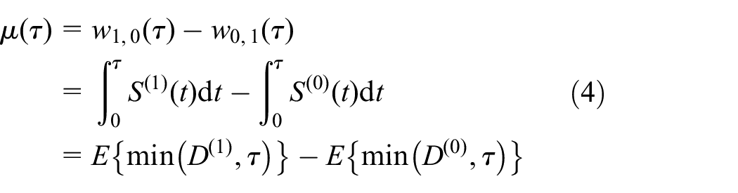
that is, the difference in RMST (net time in favor is just the extra survival time).
With multiple ranked events, the overall RMT-IF can be divided into component-specific pieces, each expressible as an integral of the component’s survival functions similarly to the second line of Equation (4).
39
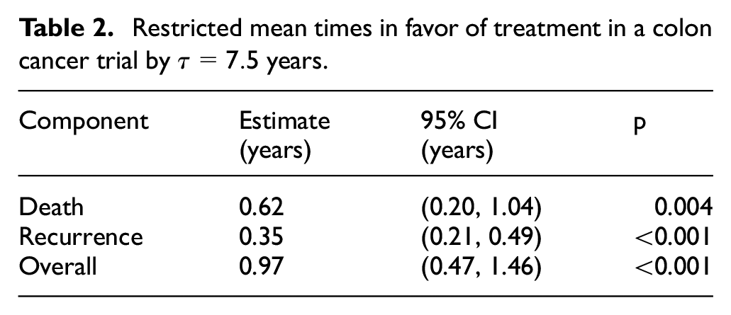
This means that we can again insert the Kaplan–Meier estimator, whose numerical stability is reliable, instead of resorting to IPCW or multiple imputations to handle censoring. As an example, consider the landmark colon cancer trial reported by Moertel et al.,
40
with death
Restricted mean times in favor of treatment in a colon cancer trial by
Temporal modeling: a semiparametric approach
A temporal model imposes a constraint on the time trajectory of certain features. A prime example is the proportionality assumption in the Cox model—group-specific hazard rates are constrained to be proportional, or equivalently their ratio constant, over time. This allows us to report the hazard ratio as a singular measure of effect size regardless of the length of follow-up. A similar strategy can be applied to the win ratio to break its dependency on the time frame.
Proportionality of win fractions (proportions)
Recall that the win–loss proportions (fractions)
To learn from the Cox model, we can posit a relationship of win and loss probabilities over time so that all data can be used. This temporal model would also obviate the need for a restriction time. The simplest idea is to posit a constant win ratio, or equivalently, proportional win and loss probabilities
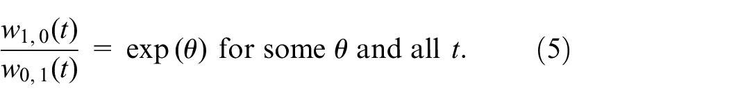
This is called the proportional win-fractions (PW) model. 43 It is semiparametric because it parametrizes only the win–loss relationship over time, while leaving other aspects of the outcomes, like the baseline event rates, unspecified. This achieves a minimal model for time-constant win ratio.
Plausibility of proportionality
Although the possibility of a constant win ratio cannot be ruled out a priori (Table 1), how plausible is it in practice? Can model (5) actually hold?
In the univariate case, we have already seen that the time-dependent win ratio on the left hand side is
Their relationship goes beyond the univariate case. In a two-tiered composite, for example, if a PH model holds not only on survival but also on the nonfatal event conditioning on survival with the same hazard ratio, then the PW model holds, again with the win ratio equal to the inverse of the (two components’ shared) hazard ratio. This extends to three components and more. In the general case, Equation (5) is implied by a Lehmann model, where the joint survival function in the treatment is equal to that in the control raised to the power of
Estimation and model diagnostics
One benefit of proportionality is that it makes estimation with censoring easier. The standard win ratio statistic, for example, is now a valid estimator of
If the model requires no modification to the standard approach, it may feel like just assuming away the problem (i.e. time dependency) to justify business as usual. However, making the assumption transparent has its own merit. Among other things, it allows us to identify when the model is violated so as not to opt for business as usual. For example, Equation (5) implies that the conditional probability of a win among determinate pairs (those excluding ties) is a constant
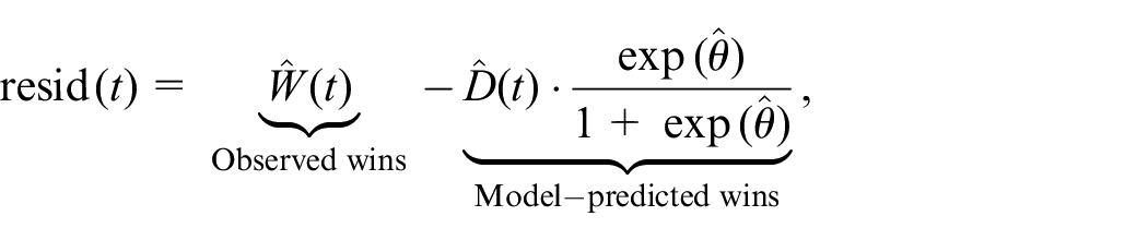
which under Equation (5) should be unbiased around zero at all times (Figure 3(a)). A closer look reveals that
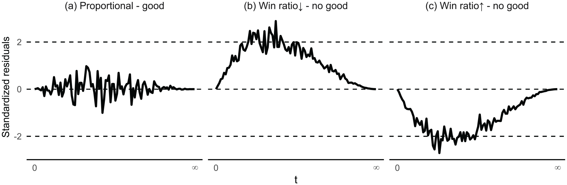
Residual processes standardized to a Brownian bridge. Extremum exceeding ± 2 suggests bias (non-proportionality).
To take a substantive view of model violations, recall that a two-tiered composite proportionality is guaranteed by a Lehmann model with a common component-wise hazard ratio. We can roughly interpret this as the treatment having the same effect on both components. This helps explain why the win ratio stays constant even as time shifts more focus to the prioritized one (Table 1). To flip the argument, when the treatment has different effects on the components, the win ratio will change magnitude to align itself more with the prioritized one as time goes on. For example, if the treatment offers a greater/smaller reduction in mortality than it does the risk of hospitalization in the survivors, the win ratio will increase/decrease, respectively, over time, making Equation (5) untenable. In such cases, the estimand of model-based estimators will be a (censoring) time-weighted average of (log-)win ratios (similarly to the partial-likelihood estimator of hazard ratio in presence of non-PH). 22 Nonetheless, it may still yield a valid test if one group wins (or loses) consistently over time compared to the other.
Covariate adjustment
Another benefit of a model like Equation (5) is that it can adjust for covariates the same way as it does the treatment arm. Let
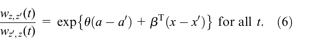
In this model,
Consider a subset of
Multiple PW regression in HF-ACTION trial.
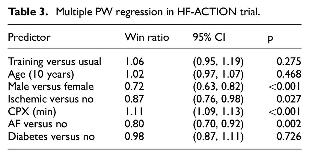
Despite the modest 6% added benefit by the treatment, multiple other factors do substantially and significantly affect patient outcomes. Of note, a mere 1-min increase in CPX test raises the likelihood of a better outcome by 11%. Would this measure of physical stamina also modify the effect of exercise training? One can find out by refitting the model with an extra treatment × CPX interaction.
Covariate adjustment by Equation (6) carries some caveats. First, the conditional win ratio is not comparable to the marginal one, where the treatment is the only predictor, due to “non-collapsibility” of the metric (average of the ratio is not ratio of the average). Second, additional predictors bring in additional assumptions, namely, that proportionality must hold for every one of them. Fortunately, similar residual processes can be used to check on each covariate. If a categorical covariate is found with a non-proportional effect, one can stratify (rather than regress) the model on it, 47 essentially restricting comparisons within each level of the strata.48–50 For two-tiered composites, PW methodology including model diagnostics and stratification is available in the WR package on CRAN. 51
Discussions
Starting a win ratio analysis by first defining the estimand clarifies the scientific goal, meets regulatory guidelines/requirements, and is after all, as we have seen, not that hard to do. In a nonparametric approach, one pre-specifies the time frame for the comparisons and deals with censored data within in an unbiased way via the use of censoring weights (IPCW). In a semiparametric approach, one constrains the win ratio to be constant regardless of the restriction time (PW model). The validity of this assumption can be checked by plotting the residuals between observed and model-predicted wins over time, whose pattern shows the actual trend of the win ratio.
Separation of estimand and estimation has limits
A clear definition of estimand benefits from separating it from estimation—the former uses the full data one wishes to observe while the latter makes do with a censored version that is actually observed. This separation is not absolute. In the nonparametric approach, for example, if the restriction time is set so far that no patient is still under observation by that time, the corresponding estimand would not be identifiable or estimable. 30 Likewise in the semiparametric approach, even if proportionality is found to be true by the observed residuals, extrapolation of the model beyond the last observation would still be a matter of faith. As a rule of thumb, a sizable portion of patients must be present at any given time in order for an estimand to be estimable or a model to be checkable with reasonable precision or confidence.
Trade-offs between two approaches
The nonparametric approach by definition has fewer assumptions, but also requires pre-specification of a restriction time and results in less data being used. The semiparametric one combines all data in a global measure of effect size, but at the price of a (somewhat stringent) temporal model. For statistical efficiency, the semiparametric approach may be preferred if its assumption is supported by the observed residuals. Otherwise, the nonparametric one offers a more robust alternative by localizing the time frame of comparison.
Improvement in efficiency and robustness
This efficiency–robustness trade-off exists largely because the current methods are still underdeveloped. An eclectic, more sophisticated approach may improve in both qualities. For example, we can define the estimand nonparametrically through time restriction, and then use semiparametric means to estimate it. In randomized trials, this often entails positing a “working model” to augment a standard estimator (e.g. IPCW) by model-based predictions of missing/censored values. This makes the estimator more efficient when the model is true, yet still unbiased when it is not (thanks to the presence of the model-free standard estimator to fall back on). 52 The same idea applies to covariate adjustment, which provides an alternative to the regression modeling of Equation (6), differing in both the estimand (marginal versus conditional) and inference (robust versus model-dependent). Although this covariate adjustment approach has been well established for standard endpoints,53–55 even with FDA recommendation, 56 using it on the win ratio faces statistical challenges, such as correlated pairs resulting from cross-group comparisons. 57
Handling of intercurrent events
With a broad brush, we have considered loss to follow-up as random censoring, a missing-data mechanism that plays no role in the estimand. This, however, should not include patient withdrawal or change of treatment due to toxicity or non-response, or what ICH E9 (R1) calls “intercurrent events”—those “occurring after treatment initiation that affect either the interpretation or the existence of the measurements associated with the clinical question of interest.” 24 Thankfully, the addendum offers some general strategies for handling such events in estimand construction, and those are instructive for the win ratio.
To start, the “hypothetical strategy” means envisioning a scenario where the composite endpoints, or at least their deduced comparison results, were observed had the intercurrent event not occurred. This is close to seeing it as “dependent censoring” and can be accommodated relatively easily within our existing frameworks. Indeed, the estimand would stay the same (with full data defined hypothetically in the absence of intercurrent event), but with changes to the estimator to correct for bias. For example, we can replace the censoring weights in the IPCW with the ones that account for the dependence of the intercurrent event on the observed data, or apply them to the estimating function of the PW model for the same purpose.
The “composite strategy” sounds even easier as it implies just adding the intercurrent event as a component to the outcome. Yet there are delicate issues to ponder, not least about which tier to insert the event and what to do with the prioritized ones that occur after it. Consider treatment failure as an intercurrent event second in importance only to death. If a patient dies after treatment failure and her survival time is used for comparison, then we are essentially following a “treatment policy strategy,” that is, intent-to-treat, for at the point of death the patient is no longer under the initial treatment she was randomized to. However, if the patient’s survival time is unknown or considered unusable after treatment failure, then we need to account for the latter as a competing risk. (Although death is also a competing risk, it poses no difficulty because it takes precedence over other components.) Different options yield different meanings to the estimand and require different approaches to estimation.
The “principal strata strategy” may be the most challenging, both conceptually and technically. It restricts the population (one of the four attributes of an estimand) to a subset defined by the potential status of an intercurrent event under different treatments. 58 More concretely, consider the principal strata of patients who would not experience treatment failure if treated. This includes not only those in the treatment group who did not experience treatment failure but also those in the control group who would not experience treatment failure if assigned otherwise. This counterfactual thinking implies a need to grapple with unobserved variables, with concomitant identifiability issues. Adding to that is the requirement that both patients under comparison in the win ratio must come from the same (counterfactually defined) stratum. Technicalities aside, the principal strata approach does have its place in causal reasoning. Besides measuring treatment effect on particular subgroups, it can help investigate treatment mechanisms. For example, the extent to which treatment effect is mediated by a biomarker can be assessed by looking at the treatment effect on patients whose biomarkers would be the same whether treated or not. 58 Win ratio-like methods framed in such counterfactual terms have only just begun to emerge.59–61 More work is certainly welcome.
Footnotes
Acknowledgements
The author thanks the Editor, Associate Editor, and an anonymous referee for their helpful comments.
Declaration of conflicting interests
The author(s) declared no potential conflicts of interest with respect to the research, authorship, and/or publication of this article.
Funding
The author(s) disclosed receipt of the following financial support for the research, authorship, and/or publication of this article: This work was supported by the National Institutes of Health (NIH; grant no. R01HL149875).