Sage Journals: Discover world-class research

Abstract

Background

The development of personalised (stratified) medicine is intrinsically dependent on an understanding of treatment-effect mechanisms (effects on therapeutic targets that mediate the effect of the treatment on clinical outcomes). There is a need for clinical trial data for the joint evaluation of treatment efficacy, the utility of predictive markers as indicators of treatment efficacy, and the mediational mechanisms proposed as the explanation of these effects.

Purpose

(1) To review the problem of confounding (common causes) for the drawing of valid inferences concerning treatment-effect mechanisms, even when the data have been generated using a randomised controlled trial, and (2) to suggest and illustrate solutions to this problem of confounding.

Results

We illustrate the potential of the predictive biomarker stratified design, together with baseline measurement of all known prognostic markers, to enable us to evaluate both the utility of the predictive biomarker in such a stratification and, perhaps more importantly, to estimate how much of the treatment’s effect is actually explained by changes in the putative mediator. The analysis strategy involves the use of instrumental variable (IV) regression, using the treatment by predictive biomarker interaction as an IV – a refined, much more powerful, and (in the present context) subtle use of Mendelian randomisation.

Conclusion

Personalised (stratified) medicine and treatment-effect mechanisms evaluation are inextricably linked. Stratification without corresponding mechanisms evaluation lacks credibility. In the presence of mediator-outcome confounding, mechanisms evaluation is dependent on stratification for its validity. Both stratification and treatment-effect mediation can be evaluated using a biomarker stratified trial design together with detailed baseline measurement of all known prognostic biomarkers and other prognostic covariates. Direct and indirect (mediated) effects should be estimated through the use of IV methods (the IV being the predictive marker by treatment interaction) together with adjustments for all known prognostic markers (confounders) – the latter adjustments contributing to increased precision (as in a conventional analysis of treatment effects) rather than bias reduction.

Introduction

After a predictive biomarker has met the necessary development milestones, it is necessary to evaluate its clinical utility through a confirmatory randomised trial [1]. It is our strongly held view that the credibility of claims concerning the utility of a predictive biomarker depends on robust trials-based evidence concerning both efficacy and treatment-effect mechanisms – that is, on evidence provided by well-designed Efficacy and Mechanisms Evaluation (EME) trials. Although one might pursue the identification and validation of a predictive biomarker as a separate objective to that of the evaluation of the mediation of treatment effects (mechanisms evaluation), we here make the case that pursuing them together (1) provides more insight into any findings arising through stratification on a predictive marker (i.e., understand the mechanisms by which different biomarker-based strata benefit from treatment) and (2) enables consistent mechanisms evaluation (by using the statistical interaction between predictive marker and treatment as a strong instrumental variable (IV) – to be explained below). Our aim in this article is to explore in some detail how biomarker information might be integrated into the design and analysis of such an EME trial to both (1) demonstrate substantial treatment-effect heterogeneity that is indicated by the predictive biomarker and (2) evaluate the treatment-effect mechanisms that are hypothesised to be the explanation for this treatment-effect heterogeneity. The work does not involve the development of new statistical methodology, but the novelty of the approach comes from its application in EME trials for the evaluation of personalised medicines. We do not undervalue the role of the traditional intention-to-treat (ITT) analysis (efficacy evaluation), but emphasise that it should be supplemented by robust evidence on treatment-effect mechanisms.

EME

A β-blocker may be effective at reducing risk of stroke in hypertensive patients, but its effect might be greater in some patients than in others. Similarly, it is likely to reduce average systolic blood pressure, and again, its effect on average blood pressure is likely to vary from one patient to another. It seems self-evident (and consistent with biological theory) that the β-blocker’s effect on risk of stroke is explained by the fact that it reduces average blood pressure. We might expect that if one individual’s blood pressure has been lowered considerably more than that of another individual, then the risk of stroke is likely to have been reduced more in the first person than in the second. But how might we evaluate these claims in a clinical trial? How might we estimate what portion of the β-blocker’s effect on stroke is explained by its effect on average blood pressure?

The rationale of the randomised clinical trial is that it enables us to conclude that differences in clinical outcomes observed in the randomised arms are valid measures of the causal effects of treatment. For simplicity, consider a randomised controlled trial with two arms: treatment versus control. Also for simplicity, we will assume that there is full adherence to the allocated treatment (relaxing this assumption does not affect the logic of our thesis, but analysis as randomised is no longer evaluating the effects of treatment receipt). Prior to randomisation to one of two competing treatment arms (supposedly active drug versus placebo control, for example) we can envisage two potential outcomes for each participant in the trial – the outcome after an active treatment, Y_A , say, and the outcome after receiving the placebo, Y_P [2,3]. We can only ever observe one of these two outcomes, dependent on the treatment assignment mechanism, with the other outcome being a counterfactual. However, in principle, we can think of the effect of treatment as a comparison of Y_A and Y_P – here, again for simplicity, we use the arithmetic difference, Y_A −Y_P . This difference defines the Individual Treatment Effect (ITE(Y)). We can never observe these individual treatment effects, of course, but the random allocation ensures that we can estimate their average:

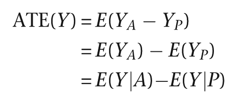
\begin{matrix} ATE (Y) = E (Y_{A} - Y_{P}) \\ = E (Y_{A}) - E (Y_{P}) \\ = E (Y | A) - E (Y | P) \end{matrix}

The Average Treatment Effect, ATE(Y), defines the efficacy of the active treatment with respect to the placebo control when the outcome of treatment is the variable Y. Efficacy is evaluated and estimated by comparison of the average of the outcomes in the two arms. Returning to the individual treatment effects, there is no reason to believe that they are the same for all participants, and in fact, there is very likely to be treatment-effect heterogeneity. This, of course, is the underlying foundation of personalised medicine.

In our randomised controlled trial, in addition to measuring the clinical outcome of obvious importance to the patient and his or her clinician, we may also choose to record the values of an intermediate or proximal outcome, M, which, based on prior biological theory, is assumed to be a strong candidate as a treatment-effect mediator (lowering systolic blood pressure lowers stroke risk, blocking certain cell receptors reduces rates of tumour growth, lowering glycosylated haemoglobin in Type 2 diabetes lowers risk of peripheral neuropathy, and so on). We assume that there is an effect of treatment on the mediator which, in turn, leads to an effect on the clinical outcome. Again, we can define an individual treatment effect for M, that is, ITE(M), and estimate the corresponding efficacy, ATE(M). And, again, there is likely to be heterogeneity of the treatment effects on the mediator, as well as those on the clinical outcome itself.

Now we turn our attention to treatment-effect mechanisms. If our intermediate outcome, M, is, in fact, a mediator of the effect of treatment on clinical outcome, Y, then we would expect that the effect of treatment on M would provide us with an explanation for its effect on Y. We are looking for more than correlation (not just association). Not only would the two effects be correlated but the effect on M would be on a causal pathway between receipt of treatment and final outcome. Complete mediation would imply that the whole of the effect of treatment on Y would be explained by its effect on M (all of the treatment’s effect on Y would be through an indirect path involving M; there would be no direct causal link between treatment and clinical outcome). More likely, however, is the fact that the effect of treatment on Y is partly explained by its effect via M; there is both a direct and an indirect causal path between treatment and outcome. This situation is represented graphically in Figure 2, and we note that both M and Y are outcomes that are indicators of response to treatment. What we wish to refer to as a mediator (the proximal outcome) or final outcome (distal to the mediator) depends upon context. Before moving on to consider these pathways further, we digress to consider treatment-effect heterogeneity in a bit more detail, particularly in the context of the development of personalised medicine.

Personalised medicine

Explicit notion of the heterogeneity of the causal effect of treatment on outcome, and the search for predictive markers that will explain this heterogeneity and be useful in subsequent treatment choice, is at the very core of what we here label as ‘Personalised Medicine’. These so-called predictive markers can arise through prior biological theory concerning mediational mechanisms or through statistical searches – but before they can be incorporated into a large clinical trial to validate their use, the preliminary evidence for their predictive role needs to be pretty convincing. If the predictive biomarker passes this preliminary hurdle, our contention is that a large trial of efficacy, designed to evaluate both treatment-effect heterogeneity and corresponding mediational mechanisms, will provide a richer and more robust foundation for personalised or stratified therapy.

Types of biomarker

In the present context, we are primarily concerned with the distinction between prognostic and predictive markers (both assumed to be measured prior to randomisation). Referring to measurements made after the onset of treatment, the third type of biomarker that would be potentially very useful is a marker of treatment activity (i.e., the putative mediator). Here, we start with definitions provided by Simon [4]: ‘A “prognostic biomarker” is a biological measurement made before treatment to indicate long-term outcome for patients either untreated or receiving standard treatment’, and ‘A “predictive biomarker” is a biological measurement made before treatment to identify which patient is likely or unlikely to benefit from a particular treatment’. Let us assume we are planning to run a placebo-controlled drug trial: supposedly active drug versus inert placebo. Here, a prognostic marker would be a marker whose average effects on patient outcome are identical in the two arms of the trial. A predictive marker (or moderator [5]), in comparison, is associated with differences in average treatment effect (it may also be prognostic in the sense that it is associated with outcome in both arms of the trial, but there would be a need to include and estimate the size of marker by treatment interactions in the model to describe the treatment outcomes (but we need to be careful to ensure that such an interaction is not simply a result of using an inappropriate model/measurement scale for the outcome). For example,

Overexpression of the HER2-neu gene in patients with early breast cancer provides an example of a biomarker that has both prognostic value (patients with HER2-neu overexpression having a worse prognosis) and predictive value for herceptin (patients with HER2-neu overexpression deriving a benefit from this treatment). [6]

Graphical representations of the effects of prognostic and predictive biomarkers are illustrated in Figures 1(a) and 1(b), respectively.

Figure 1.

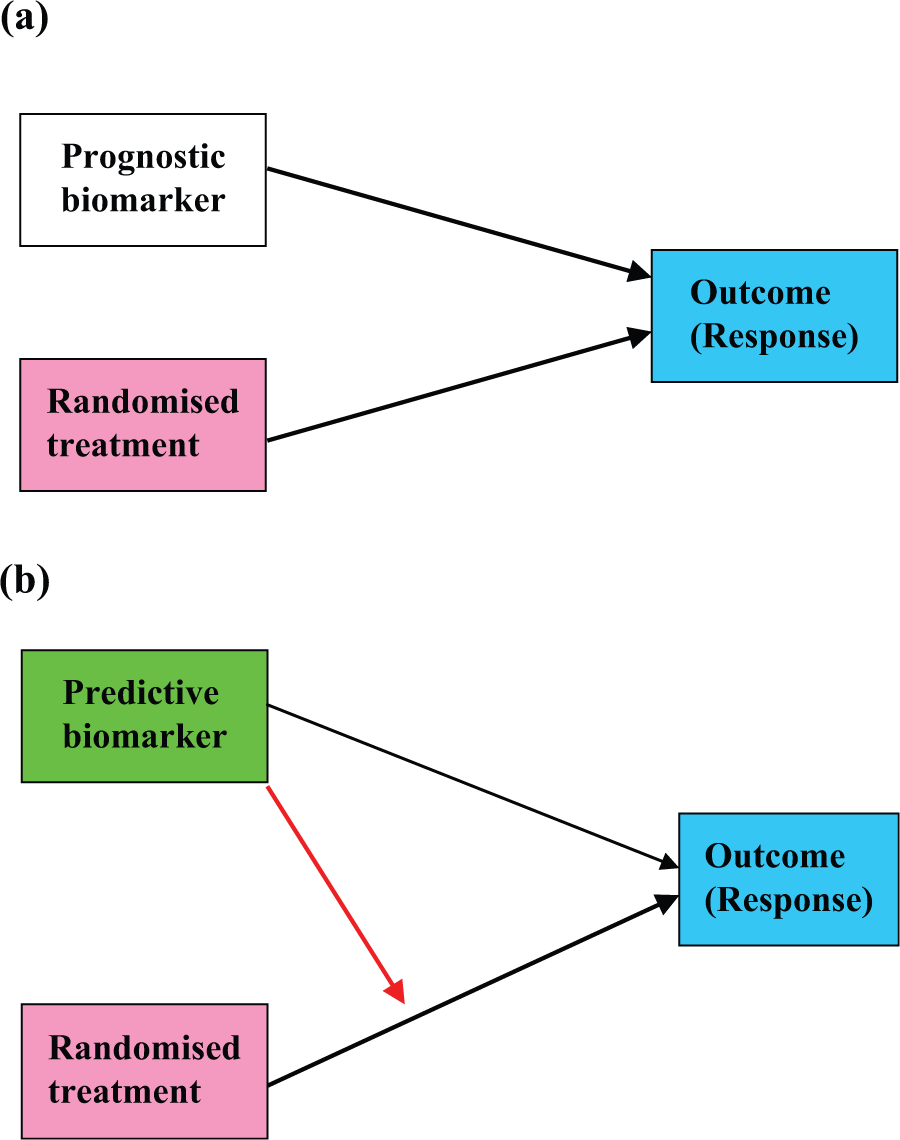
Graphical representations of the effects of prognostic and predictive biomarkers: (a) prognostic biomarker and (b) predictive biomarker.

Models for mediation

A simple graphical representation of treatment-effect mediation is shown in Figure 2(a). Treatment has an effect on the mediator which, in turn, has an effect on the outcome (this is the indirect pathway). Treatment also has a direct effect on outcome (i.e., that portion of the treatment’s effect that is not explained by the postulated mediational mechanism). However, Figure 2(a) is labelled as ‘naïve’. Why? In the critical appraisal of postulated causal diagrams, one should always be very wary of what might have been omitted. Omitted common causes (hidden confounding) should always be considered as a possible explanation for associations that might be interpreted as causal. Random allocation of treatment (assuming, of course, complete adherence to the treatment allocation) first rules out any common causes for treatment and the mediator and, second, rules out any common causes for treatment and the clinical outcome. But neither mediator nor clinical outcome are under the direct control of randomisation and there are very likely to be factors, other than treatment, that have a common influence on these two outcomes of treatment. If we were to assume that the model specified by Figure 2(a) is the correct one and analyse the data accordingly (as described in the highly cited article by Baron and Kenny [7], for instance), then we are very likely to obtain misleading (biased) results if such omitted common causes of mediator and outcome do exist.

Figure 2.

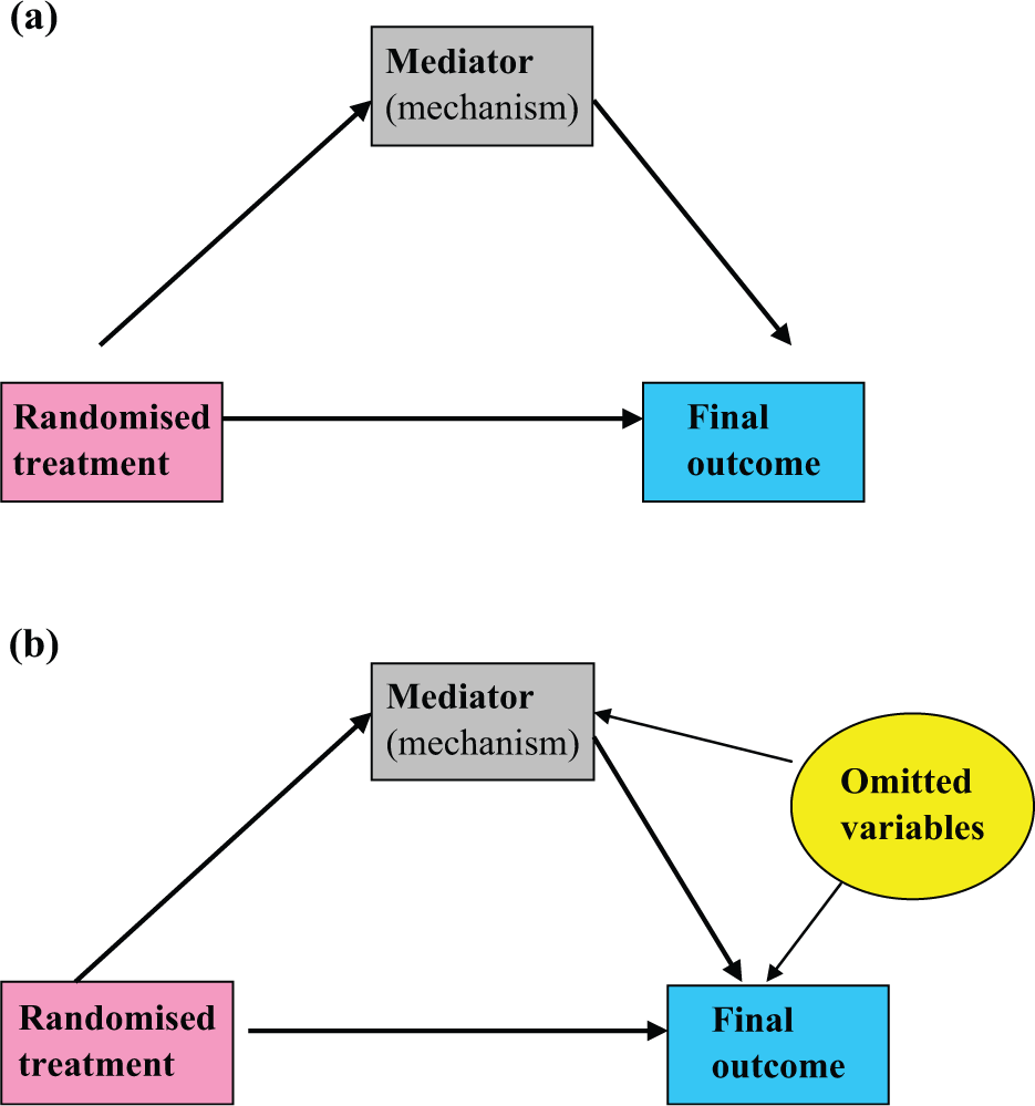
Graphical representation of mediation: (a) the naïve model and (b) acknowledging hidden common causes (confounders).

A more realistic model is represented by Figure 2(b). We have added the effects of the omitted pre-randomisation variables (these are represented by convention within an elliptical frame – indicating a latent variable). Again, a key feature concerns connections that are missing. There is no link between the omitted variables and treatment, and specifically, there is no effect of treatment on any of these omitted variables. How do we analyse our data to estimate direct and indirect treatment effects when assuming this model to be the correct one? Unfortunately, we cannot, without incurring bias. If we only have data on treatment allocation, and the values of the two outcome measures (mediator and final outcome), then we have a real problem. There is not enough information contained in the data to allow us to estimate the required treatment effects in the presence of hidden confounding. Statisticians describe this situation as an identifiability problem: the model is said to be under-identified. In implementing our trial, we need to collect more data – and this is where biomarker measurements come in. The potentially important roles of prognostic markers will be discussed in the sections ‘Using prognostic markers for confounder adjustment’ and ‘Using prognostic markers as IVs (Mendelian randomisation)’, and then we move on to discuss the even more important role of predictive markers.

Before leaving this section, we admit to another simplifying (‘naïve’) assumption which is shared by the Baron and Kenny model [7]. We are ignoring the problem of measurement errors in the mediator and the final outcome. This does not matter in the case of the final outcome (except for lowering the precision of the estimated treatment effects), but measurement errors in the mediator can lead to serious biases. We will return to this potential complication later when we show that the analytical solution of the hidden confounding problem also deals with those arising from random measurement errors in the mediator.

Using prognostic markers for confounder adjustment

Independent of treatment, baseline (pre-randomisation) prognostic markers are related to outcome. A prognostic marker may have, and is likely to have, an effect on both the intermediate and clinical outcomes. If so, then it is a confounder. If we measure and record the value of the prognostic variable, then we are in a position to allow for its effects in our analyses. If we take measurements on several prognostic biomarkers and other baseline covariates thought to have prognostic value, then the resulting model is as in Figure 3(a). In a two-stage analysis we first estimate the effect of treatment on the mediator, adjusting for all of our additional measurements (baseline covariates and prognostic biomarkers), and then we look at the joint effects of mediator and treatment on outcome, again adjusting for all of our measured confounders (baseline covariates and prognostic biomarkers). This two-stage procedure will be valid if and only if we have accounted for all of the common causes of M and Y. Otherwise the effects we are attempting to estimate will suffer from residual confounding (residual biases). There may be baseline markers that we might have measured, but have not – we may be unaware of their existence, for instance – and there are likely to be events (common causes) influencing the participant once treatment has been initiated (post-randomisation confounders – infections, bereavements, accidents and other life events; co-morbid illness; additional medications; etc.). We can never be sure.

Figure 3.

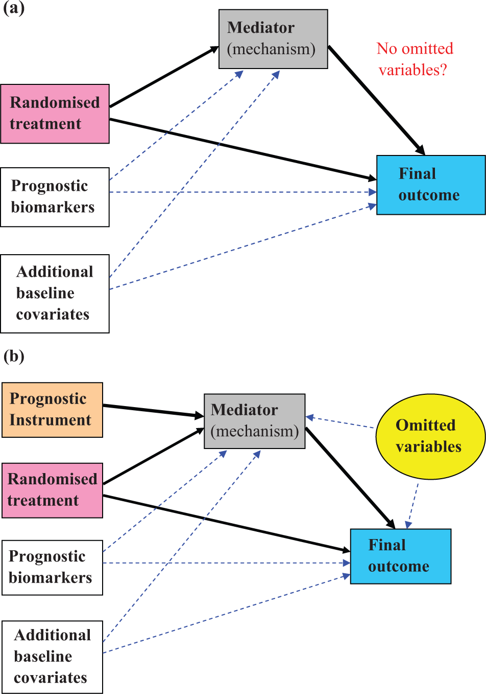
Making the most of the prognostic marker information: (a) adjustment for all measured confounders (including prognostic markers) and (b) introducing an instrumental variable (as in Mendelian randomisation).

Using prognostic markers as IVs (Mendelian randomisation)

What if we have prior biological knowledge which makes it highly plausible that a particular prognostic marker has an effect on the mediator and, although it is related to clinical outcome, it has no direct effect on the clinical outcome? If this were the case and the marker was also uncorrelated with the omitted common causes, then such a prognostic marker would be what is known as an IV or, in short, an instrument. We do not wish to discuss any of the technical details here, but such a situation would enable us to use statistical techniques based on IV models in order to obtain unbiased estimates of the direct and indirect effects of treatment in the presence of hidden confounding (including common causes arising post-randomisation). The IV method also eliminates biases arising from random measurement error in the putative mediator. The avoidance of bias, however, comes at a cost. We are losing precision when using IV methods. If the prognostic biomarker were a genetic variant, then this IV technique is an example of what has been called Mendelian randomisation [8,9] –‘Mendelian’ because we are dealing with genetic variation; ‘randomisation’ because of the random assortment of alleles during gamete formation. The causal model involving a prognostic instrument – such as Mendelian randomisation – is illustrated in Figure 3(b)

Assuming that we are prepared to exchange lower precision for lack of bias, why should we not decide that we now have the solution? What are the limitations of Mendelian randomisation in the context of randomised trials for mechanisms evaluation? The first is that in order to be of real practical value, the instrument has to have a strong effect on the putative mediator. In the context of a randomised trial specifically focussing on an intervention targeting the proposed mediator, genes are likely to explain very little of the within-treatment variability of the mediator. This is the so-called weak instrument problem [10,11]. If we have weak instrments, the treatment-effect estimates are very imprecise, and worse than that, they are inconsistent – they are likely to be biased even with very large sample sizes [10,11]. Another potential problem is that the assumption of no direct effect of the genetic variation on clinical outcome (i.e., that there are no other mediators of the treatment effect) may be untenable [12]. We want to be fairly confident that our identifying assumptions (those needed to allow us to estimate the relevant treatment-effect parameters without bias) are not obviously open to challenge. In this context, it will be practically impossible to verify them using the data at hand.

Using predictive markers to generate IVs

Remembering that a predictive marker also has prognostic properties, a predictive marker is likely to be a confounder. In itself, it is unlikely to be a valid instrument. But what about the treatment-effect moderation (the treatment by marker interaction)? The very essence of predictive (stratified) medicine is that there is very strong moderation by the predictive marker of the treatment effect on a supposedly known target mechanism (mediator) and that the moderating effect of predictive marker on the clinical (distal) outcome is explained by treatment-induced changes in the mediator. Accepting these conditions (assumptions) is equivalent to stating that the treatment by predictive marker interaction is an IV. This is a strong assumption, always open to challenge, but weaker and more easily defended than those needed for Mendelian randomisation (see above). For example, trastuzumab is a highly specific monoclonal antibody targeted on the HER2-neu receptor protein, and its efficacy is claimed to be moderated by the genetic marker associated with variation in baseline levels of the HER2-neu receptor. The assumption that the treatment (trastuzumab) by genotype interaction is a valid instrument seems eminently plausible. The additional assumption that the HER2-neu genotype, itself, does not have a direct effect on clinical outcome is stronger, and may be much less plausible.

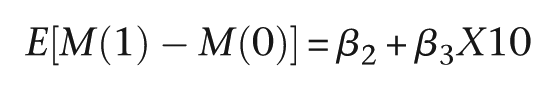
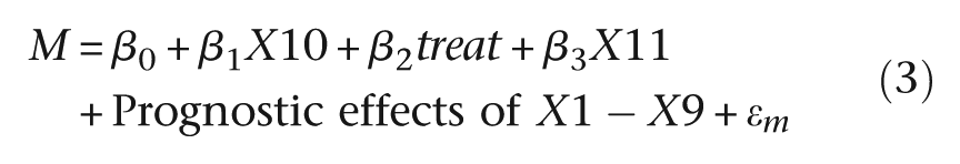
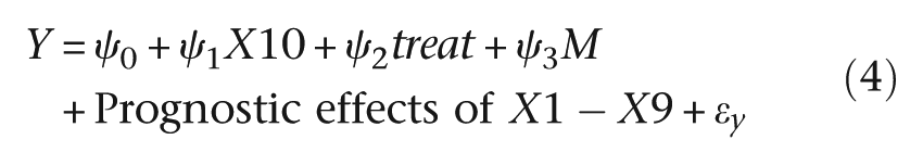
Let the binary treatment be represented by the variable treat. Anticipating our simulated EME trial (to be described below), let a binary predictive marker be X10 and the product of treat and X10 be X11. The two causal (structural) models are

M = β_{0} + β_{1} X 10 + β_{2} treat + β_{3} X 11 + ε_{m}

(1)

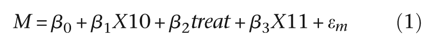
that is

E [M (1) - M (0)] = β_{2} + β_{3} X 10

Y {= Ψ}_{0} {+ Ψ}_{1} X 10 + Ψ_{2} treat + Ψ_{3} M + ε_{y}

(2)

that is

E [(Y (1) - Y (0)) | X 10] = Ψ_{2} {+ Ψ}_{3} E [(M (1) - M (0)) | X 10]

where ϵ_m and ϵ_y are the random deviations (‘errors’) associated with each of the two models, respectively. We assume that these errors are correlated; that is, cov(ϵ_m, ϵ_y ) ≠ 0, acknowledging the fact that there are missing common causes of M and Y. β ₂ is the effect of treatment on the mediator (M) when X10 = 0. β ₃ is a measure of the strength of the effect on the mediator of the interaction between treatment and predictive biomarker. The effect of the treatment on the mediator when X10 = 1 is the sum of β ₂ and β ₃. The direct effect of treatment on outcome (Y) is the parameter ψ ₂, and the effect of the mediator on outcome (irrespective of the levels of treatment and X10) is ψ ₃. β ₁ and ψ ₁ are of no intrinsic interest but are included to allow for the confounding explained by the predictive marker, X10.

The total effect of treatment on outcome when X10 = 0 is simply β ₂ ψ ₃+ψ ₂, and the proportion explained by its effect on the mediator is β ₂ ψ ₃/(β ₂ ψ ₃+ψ ₂). Similarly, the total effect of treatment when X10 = 1 is (β ₂+β ₃)ψ ₃+ψ ₂, and the proportion explained by its effect on the mediator is (β ₂+β ₃)ψ ₃/((β ₂+β ₃)ψ ₃+ψ ₂).

Is our assumption that the interaction (X11) is a valid IV justified? This depends on the strength of the biological theory and the supporting evidence for considering X10 to be a good predictive marker. Is the interaction (X11) likely to be a weak instrument? No. If it were a weak instrument (i.e., a weak moderator) then we would suggest that it would have already been discarded as a potentially useful stratifying marker. For a predictive biomarker to have met the necessary development milestones implies that it is confidently assumed to be a powerful moderator of the effect of the treatment on the proposed mediator. We are suggesting a refined, much more powerful, and (in the present context) useful version of Mendelian randomisation.

Taking equations (1) and (2) to represent the core feature of an EME trial for a personalised treatment, we now integrate all of our potential biomarker measurements to suggest a viable trial design and associated data analysis strategy.

Putting it all together: a suggested Biomarker Stratified Efficacy and Mechanisms Evaluation (the BS-EME) trial and associated analysis strategy

In the marker by treatment interaction design, we stratify patients according to marker status and randomise to treatments within each marker stratum [1]. An alternative phrase to describe this design is ‘biomarker stratified design’ [4,13]. We are concerned with evaluating whether the treatment effects are the same in the different strata. In the present context, our stratifying biomarker is the binary variable, X10. Here, we assume that we are planning a new trial but, of course, the same principles might be applied to a retrospective analysis of archived trial data (or the meta-analysis of individual patient data from several trials); however, we would be pleasantly surprised if a rich-enough data set was available for such an analysis.

Taking the biomarker stratified design as described above, we supplement the baseline information (i.e., X10 status) by measuring all previously validated prognostic markers (X1–X9, say) together with baseline covariates (demographic information; clinical and treatment history; co-morbidity; social, psychological and cultural variables; and so on) thought to have prognostic value. One obvious covariate is the baseline measurement of the putative mediator. Another might be a baseline value for the final outcome measurement. The rationale for all of these measurements is (1) to allow for as much confounding of the effects of the mediator on final outcome as is feasible, (2) to assess sensitivity of the results to assumptions concerning residual hidden confounding and, perhaps more importantly, and (3) to increase the precision of the estimates of the important causal parameters (as described in the section ‘Using predictive markers to generate IVs’).

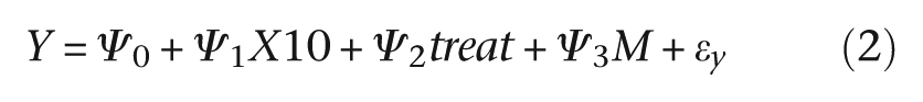
The graphical representation of the causal influences to be estimated from data arising from our proposed design is shown in Figure 4. The two main components of the model are (1) that for the combined effects of treatment, markers and covariates on the mediator (including the treatment by predictive marker interaction), and (2) that for the combined effects of treatment, mediator, markers and covariates on the final outcome (but with no treatment by predictive biomarker interaction). Again, we bear in mind the hidden confounding. These two regression models can be fitted simultaneously with ease using two-stage least-squares (2sls) – a so-called IV regression [14], available in most general-purpose statistical software packages. Essentially, we are simultaneously fitting our data to both equations (1) and (2) after adjusting for all measured confounders. We illustrate these analyses in the section ‘Illustrative example: a simulated BS-EME trial’.

Figure 4.

Using the predictive marker by treatment interaction as an instrumental variable – using all available information (the BS-EME trial).

Illustrative example: a simulated BS-EME trial

At this point, it would be nice to be able to illustrate our ideas by reference to the analysis of data from a real trial. Unfortunately, we are not aware of the existence of trial(s) providing data along the lines advocated here, and we do not have access to any archived trial data that might be used as a suitable illustration. In the United Kingdom, funding for EME trials is a very recent innovation (http://www.eme.ac.uk/) and few, if any of these trials have reached completion. The application of EME methodology to personalised medicine is in its infancy. We are not aware of similar EME programmes in the United States or elsewhere. Therefore, we have resorted to a Monte Carlo simulation – the one big advantage here being that we know the answers! Both the simulation and the illustrative analyses were carried out in Stata version 11 [15].

We simulate a relatively small trial with 100 participants randomly allocated to each of two arms. We have baseline (pre-randomisation) measurements of nine binary prognostic markers (X1–X9) on all participants – genetic markers, say, with varying allele frequencies (details are provided in the Appendix A). We postulate a normally distributed quantitative mediator (M) and, similarly, a normally distributed indicator of final outcome (Y). The presence of each of the prognostic alleles coded as 1 increases both the mediator and the outcome by five units (i.e., these prognostic markers are all confounders of the effect of M on Y). We now introduce the randomised treatment (treat), together with a binary (0/1) predictive biomarker, X10, with the prevalence of the variant coded as 1 being 20%, again measured prior to randomisation. As before, the product of X10 and treat, X11, is the statistical interaction that measures the strength of the moderation of the treatment effect by X10. The marker X10 itself has a prognostic effect on both M and Y (i.e., it too is a confounder). If we allow appropriately for X1–X11 in our statistical analyses of the resulting data, there will be no hidden confounding (no omitted variables effects).

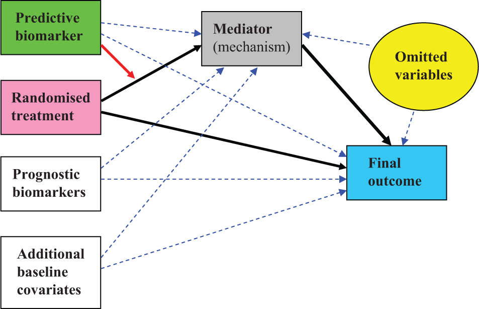
Therefore, the statistical (causal) models used to generate the data are

\begin{matrix} M & = β_{0} + β_{1} X 10 + β_{2} treat + β_{3} X 11 \\ + Prognostic effects of X 1 - X 9 + ε_{m} \end{matrix}

(3)

\begin{matrix} Y & = ψ_{0} + ψ_{1} X 10 + ψ_{2} treat + ψ_{3} M \\ + Prognostic effects of X 1 - X 9 + ε_{y} \end{matrix}

(4)

Full details are given in the Appendix A. Here, all we need to know are the true values of β ₂ and β ₃, and of ψ ₂ and ψ ₃. They are 5, 20, 10 and 2, respectively. A value of 20 for β ₃ may appear to be unusually high, but for a predictive biomarker to have met the necessary development milestones implies that is a powerful moderator of the effect of the treatment on the proposed mediator. Summary statistics for this simulated trial are given in Table 1(a), and the results of two simple regressions illustrating the joint effects of treatment and predictive marker on the two outcomes (M and Y, separately), together with their expected (true parameter) values, are shown in Table 1(b). Note that these estimates obtained using models with no reference to the prognostic markers, X1–X9, are not confounded – we are simply looking at the ITT effects of randomisation in the two strata determined by the values of the predictive marker (X10). However, if we were to adjust for the effects of X1–X9 in our analyses, then there would be a gain in precision.

Table 1.

A simulated BS-EME trial

(a) Summaries of the outcomes in our simulated trial: by predictive biomarker and treatment
Biomarker	Treatment	No. obs	Mean (M)	s.d. (M)	Mean (Y)	s.d. (Y)
0	No (0)	79	72.655	8.087	167.79	22.994
0	Yes (1)	80	77.732	8.449	188.5	22.402
1	No (0)	21	77.93	7.639	185.194	22.701
1	Yes (1)	20	103.21	6.866	244.025	18.213

(b) Standard regressions to test for interactions (the effect of X11)

	Regress m X10 treat X11			Regress y X10 treat X11
Effect	Expected*	Estimate	s.e.	Expected*	Estimate	s.e.

X10	+5	+5.275	1.984	+15	+17.404	5.476
treat	+5	+5.077	1.282	+20	+20.71	3.538
X11 (i.e., interaction)	+20	+20.203	2.832	+40	+38.12	7.815

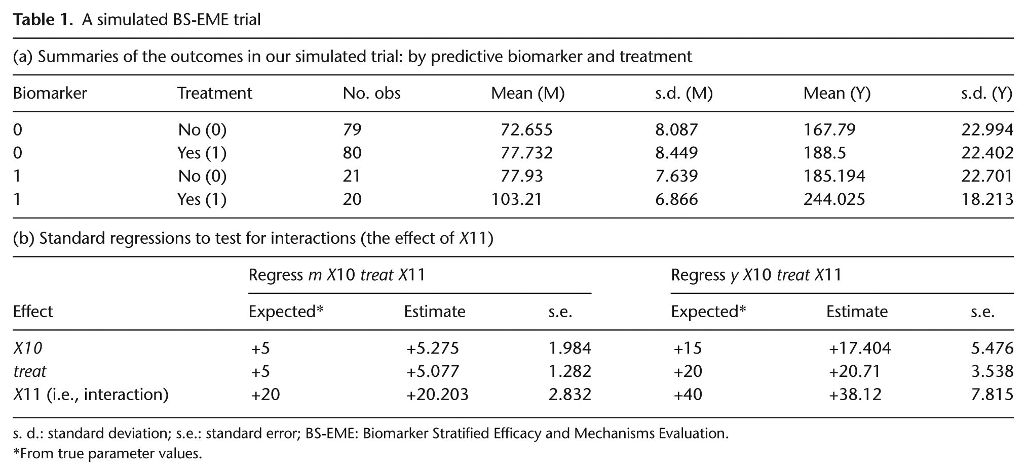
s. d.: standard deviation; s.e.: standard error; BS-EME: Biomarker Stratified Efficacy and Mechanisms Evaluation.

From true parameter values.

Returning to our true model (equations (3) and (4)), when X10 = 0, the overall (total) effect of treatment on final outcome (Y) is 20 units, and the expected (true) proportion of the treatment effect on Y that is explained by its effect on M (i.e., the indirect effect of treatment) is (5 × 2)/20 × 100% = 50%. When X10 = 1, the total effect is 60 units, and the true proportion explained by treatment-induced changes in M is (25 × 2)/60 × 100% = 83%. The question we now pose is ‘What analysis do we need to retrieve unbiased estimates of these effects?’ Estimating the joint effects of treatment and X10 on M, and of their interaction X11, is not a problem, even in the absence of data on the prognostic markers. Estimating the joint effects of treatment X10 and M on the outcome, Y, however, is another matter. Table 2(a) shows the results of fitting the corresponding regression models (the naïve model – as in the Baron and Kenny strategy [7]) in three situations. First (on the left), we assume that we have no measures on any of the prognostic markers (or we have chosen not to use the data). Second (in the centre), we have data on and have adjusted for four of them (X1–X4). Finally (on the right), we have made adjustments for the effects of all nine of prognostic markers. The results on the left are clearly biased, and only some of the bias has been corrected by allowance for X1–X4. Without adjusting for any confounding, the portions of the treatment effects explained by M are 69% and 92% when X10 = 0 and X10 = 1, respectively. After adjusting for all nine confounders, the estimated portions are 51% and 82%, respectively – demonstrating that if we know all the confounders and if we make adjustments for them all, then we can retrieve the correct treatment effects.

Table 2.

Multiple regression models for the joint effects of treatment and the mediator on outcome

(a) No interactions
		Naïve model (regress y X10 treat m)		Adjustment for X1–X4 (regress y X10 treat m X1 X2 X3 X4)		Adjustment for all confounders (regress y X10 treat m X1 X2 X3 X4 X5 X6 X7 X8 X9)
Effect	Expected*	Estimate	s.e.	Estimate	s.e.	Estimate	s.e.
X10	+5	−1.643	1.493	+0.999	1.478	+6.009	1.286
treat	+10	+5.613	1.119	+7.534	1.104	+11.859	0.971
M	+2	+2.485	0.055	+2.334	0.059	+1.962	0.058

(b) Including a treatment by predictive marker interaction (i.e., the effect of X11)

		Naïve model (regress y X10 treat m X11)		Adjustment for X1–X4 (regress y X10 treat m X11 X1 X2 X3 X4)		Adjustment for all confounders (regress y X10 treat m X11 X1 X2 X3 X4 X5 X6 X7 X8 X9)
Effect	Expected*	Estimate	s.e.	Estimate	s.e.	Estimate	s.e.

X10	+5	+3.474	1.622	+4.237	1.578	+6.449	1.355
treat	+10	+7.302	1.070	+8.324	1.066	+2.013	0.971
M	+2	+2.641	0.057	+2.497	0.067	+2.013	0.077
X11		−15.231	2.552	−11.890	2.621	−2.516	2.440

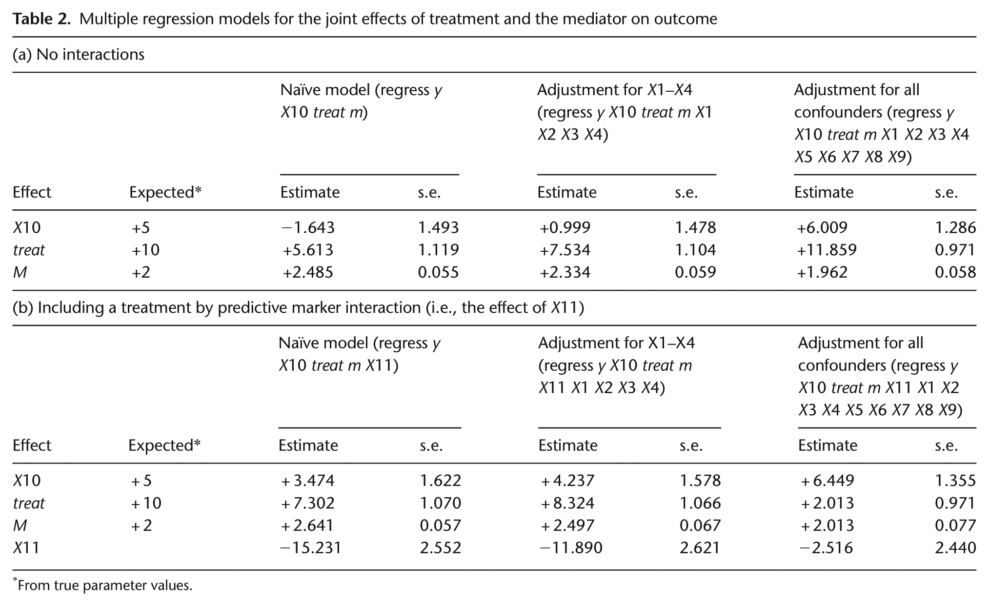
From true parameter values.

So far, none of our analysis models for the joint effects of M and treatment on the final outcome Y have included a treatment by X10 interaction. Our trial will have been designed on the assumption that such an interaction does not exist. Our data have here been simulated without this interaction. What if we naïvely try to use our data to test whether this interaction actually exists? The results of these analyses are shown in Table 2(b). The two naïve analyses reveal a highly statistically significant interaction. This is an artefact of confounding. Only if we correctly allow for all of the known confounders (the column on the right) do we obtain a small and statistically non-significant effect.

The use of familiar analyses based on multiple regression has illustrated the problem of the confounding of the effect of the mediator on final outcome. Only when we have measured and allowed for all of the prognostic variables that explain this confounding can we be confident in our results, including an evaluation of whether there is a direct effect of the treatment by predictive marker interaction (X11) on the final outcome (i.e., whether X11 is a valid IV). In reality, even when we have collected data on and allowed for all known confounders, we will not know whether there is any residual confounding. Which is the safer assumption – (1) there is no hidden confounding, or (2) there is no direct effect of X11 on final outcome (X11 is a valid instrument)? If our biological knowledge is as firm as many investigators appear to claim it to be, then we would be far more confident in (2).

Finally, assuming that X11 is indeed a valid IV, we illustrate the use of IV regression (using 2sls, for example) to analyse our data. The results are given in Table 3: on the left without using X1–X9, and on the right after allowing for X1–X9 as measured confounders. First, note the similarity of the estimates from the two analyses. The validity of the simple analysis on the left is not dependent on X1–X9. The main difference is that after we allow for these variables, the standard errors of the estimates are considerably lower (about 60% lower in this example). This has implications for trial size and might make the difference between a viable trial and one that is not practically feasible. The IV regression without covariates indicates that the portion of the treatment effect on Y explained by its effect on M is 46% and 81% when X10 = 0 and X10 = 1, respectively. After adjustment for all covariates, the figures are 48% and 80%, respectively.

Table 3.

Instrumental variable estimators

		No prognostic markers in the analysis model (ivregress 2sls y X10 treat (m = X11))		All prognostic markers in the analysis model (ivregress 2sls y X1 X2 X3 X4 X5 X6 X7 X8 X9 X10 treat (m = X11))
Effect	Expected*	Estimate	s.e.	Estimate	s.e.
First-stage regressions (modelling M)
X10	+5	+5.275	1.984	+4.968	1.235
treat	+5	+5.077	1.282	+6.202	0.803
X11	+20	+20.203	2.832	+20.612	1.762

Second-stage regressions (modelling Y)
X10	+5	+7.451	2.784	+7.056	1.590
treat	+10	+11.130	1.878	+12.599	1.172
X11	+2	+1.887	0.153	+1.891	0.087

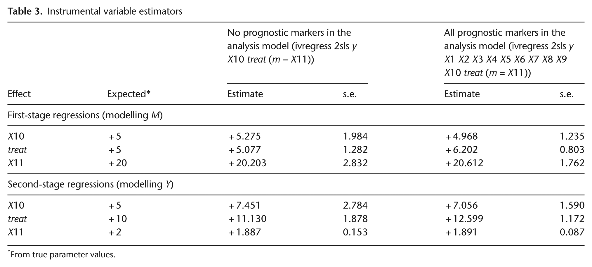
From true parameter values.

Comparing the results presented in Table 2 with those in Table 3, it is clear that the IV estimates are less precise, even in the situation where we have adjusted for all of the confounders – in this latter situation, the acknowledgement that there may be hidden confounding (even though we know that in this case there is not) is reflected in a less precise estimate. In moving from ‘conventional’ regression models involving adjustment for all measured confounders to the corresponding IV model, we assume that we are reducing bias (correct if there is residual hidden confounding), but we are reducing bias at the cost of decreased precision. We suggest that trial investigators specify one of the two approaches as the primary analysis and then include the other one as part of a secondary analysis of the sensitivity of the findings to various model assumptions.

Technical issues

Readers interested in a more technical discussion of the methods that can be used to estimate the direct and indirect (mediated) effects of treatments in randomised trials are referred to the relevant statistical literature [16 –22].

Conclusion

We conclude with a series of simple statements aimed at encouraging trialists to seriously consider the role of biomarkers that enable the simultaneous evaluation of the utility of a putative predictive biomarker and the treatment-effect mechanisms motivating its use.

Personalised (stratified) medicine and treatment-effect mechanisms evaluation are inextricably linked.

Stratification without corresponding mechanisms evaluation lacks credibility.

In the almost certain presence of mediator-outcome confounding, mechanisms evaluation is dependent on stratification for its validity.

Both stratification and treatment-effect mediation can be evaluated using a biomarker stratified trial design together with detailed baseline measurement of all known prognostic biomarkers and other prognostic covariates.

Direct and indirect (mediated) effects should be estimated through the use of IV methods (the IV being the predictive marker by treatment interaction) together with adjustments for all known prognostic markers (confounders) – the latter adjustments contributing to increased precision (as in a conventional analysis of treatment effects) rather than bias reduction.

Footnotes

Appendix A

Funding

This work was supported by the UK Medical Research Council (grant number G0900678) and a Medical Research Council Career Development Award (to R.E.). S.L. was supported by the NIHR Biomedical Research Centre for Mental Health at South London, Maudsley NHS Foundation Trust and King’s College London.

Conflict of interest

The views expressed are those of the authors and not necessarily those of the NHS, the NIHR or the Department of Health.

References

Young

Laird

Zhou

. The efficiency of clinical trial designs for predictive biomarker validation. Clin Trials 2010; 7: 557–66.

Rubin

. Estimating causal effects of treatment in randomized and nonrandomized studies. J Educ Psychol 1974; 66: 688–701.

Holland

. Statistics and causal inference. J Am Stat Assoc 1986; 81: 945–60.

Simon

. Clinical trials for predictive medicine: New challenges and paradigms. Clin Trials 2010; 7: 516–24.

Kraemer

Fairburn

Agras

. Mediators and moderators of treatment effects in randomized clinical trials. Arch Gen Psychiatry 2002; 59: 877–83.

Buyse

. Towards validation of statistically reliable biomarkers. Eur J Cancer Suppl 2007; 5: 89–95.

Baron

Kenny

. The moderator-mediator variable distinction in social psychological research: Conceptual, strategic, and statistical considerations. J Pers Soc Psychol 1986; 51: 1173–82.

Smith

Ebrahim

.‘Mendelian randomisation’: Can genetic epidemiology contribute to understanding environmental determinants of disease? Int J Epidemiol 2003; 32: 1–22.

Lawlor

Harbord

Sterne

JAC

. Mendelian randomisation: Using genes as instruments for making causal inferences in epidemiology. Stat Med 2008; 27: 1133–63.

10.

Burgess

Thompson

. Avoiding bias from weak instruments in Mendelian randomisation studies. Int J Epidemiol 2011; 40: 755–64.

11.

Burgess

Thompson

. Bias in causal estimates from Mendelian randomisation studies with weak instruments. Stat Med 2011; 30: 1312–23.

12.

Didelez

Sheehan

. Mendeleian randomisation as an instrumental variable approach to causal inference. Stat Methods Med Res 2007; 16: 309–30.

13.

Freidlin

McShane

Korn

. Randomized clinical trials with biomarkers: Design issues. J Natl Cancer Inst 2010; 102: 152–60.

14.

Angrist

Pischke

J-S

. Mostly Harmless Econometrics: An Empiricist’s Companion. Princeton University Press, NJ, 2009.

15.

Stata Corporation. Stata Version 11. Stata Corporation, College Station, TX, 2009.

16.

Ten Have

Joffe

Lynch

. Causal mediation analysis with rank preserving models. Biometrics 2007; 63: 926–34.

17.

Dunn

Bentall

. Modelling treatment-effect heterogeneity in randomized controlled trials of complex interventions (psychological treatments). Stat Med 2007; 26: 4719–45.

18.

Albert

. Mediation analysis via potential outcomes models. Stat Med 2008; 27: 1282–304.

19.

Emsley

Dunn

White

. Mediation and moderation of treatment effects in randomised controlled trials of complex interventions. Stat Methods Med Res 2010; 19: 237–70.

20.

Ten Have

Joffe

. A review of causal estimation of effects in mediation analyses. Stat Methods Med Res 2012; 21: 77–107.

21.

Clarke

Windmeijer

. Instrumental variable estimators for binary outcomes. Working Paper no. 09/209, January 2009. Bristol: Centre for Market and Public Organisation, University of Bristol.

22.

Palmer

Sterne

JAC

Harbord

. Instrumental variable estimation of causal risk ratios and causal odds ratios in Mendelian randomization analyses. Am J Epidemiol 2011; 173: 1392–403.

Integrating biomarker information within trials to evaluate treatment mechanisms and efficacy for personalised medicine

Abstract

Background

Purpose

Results

Conclusion

Introduction

EME

Personalised medicine

Types of biomarker

Models for mediation

Using prognostic markers for confounder adjustment

Using prognostic markers as IVs (Mendelian randomisation)

Using predictive markers to generate IVs

Putting it all together: a suggested Biomarker Stratified Efficacy and Mechanisms Evaluation (the BS-EME) trial and associated analysis strategy

Illustrative example: a simulated BS-EME trial

Technical issues

Conclusion

Footnotes

Appendix A

Funding

Conflict of interest

References