
Abstract
Background
On-site source data verification is a common and expensive activity, with little evidence that it is worthwhile. Central statistical monitoring (CSM) is a cheaper alternative, where data checks are performed by the coordinating centre, avoiding the need to visit all sites. Several publications have suggested methods for CSM; however, few have described their use in real trials.
Methods
R-programs were created to check data at either the subject level (7 tests within 3 programs) or site level (9 tests within 8 programs) using previously described methods or new ones we developed. These aimed to find possible data errors such as outliers, incorrect dates, or anomalous data patterns; digit preference, values too close or too far from the means, unusual correlation structures, extreme variances which may indicate fraud or procedural errors and under-reporting of adverse events. The methods were applied to three trials, one of which had closed and has been published, one in follow-up, and a third to which fabricated data were added. We examined how well the methods work, discussing their strengths and limitations.
Results
The R-programs produced simple tables or easy-to-read figures. Few data errors were found in the first two trials, and those added to the third were easily detected. The programs were able to identify patients with outliers based on single or multiple variables. They also detected (1) fabricated patients, generated to have values too close to the multivariate mean, or with too low variances in repeated measurements, and (2) sites which had unusual correlation structures or too few adverse events. Some methods were unreliable if applied to centres with few patients or if data were fabricated in a way which did not fit the assumptions used to create the programs. Outputs from the R-programs are interpreted using examples.
Limitations
Detecting data errors is relatively straightforward; however, there are several limitations in the detection of fraud: some programs cannot be applied to small trials or to centres with few patients (<10) and data falsified in a manner which does not fit the program’s assumptions may not be detected. In addition, many tests require a visual assessment of the output (showing flagged participants or sites), before data queries are made or on-site visits performed.
Conclusions
CSM is a worthwhile alternative to on-site data checking and may be used to limit the number of site visits by targeting only sites which are picked up by the programs. We summarise the methods, show how they are implemented and that they can be easy to interpret. The methods can identify incorrect or unusual data for a trial subject, or centres where the data considered together are too different to other centres and therefore should be reviewed, possibly through an on-site visit.
Introduction
Substantial resources are spent conducting clinical trials, due in part to current guidelines and regulations. International Conference on Harmonisation–Good Clinical Practice (ICH-GCP) [1] requires that the data be ‘accurate, complete, and verifiable from source documents’. A statement adhered to by many organisations is, ‘In general there is a need for on-site monitoring, before, during, and after the trial’. Although site visits can be useful to examine procedures for safety reporting and drug labelling, for verifying pharmacy supplies, and performing other monitoring tasks, considerable effort is typically spent checking trial data with patient records, i.e., source data verification. Although some organisations use source data verification for a random sample of participants (e.g. 20%), others still perform 100% checks. A clinical trial database can never be completely free from errors. Monitoring of trial data is used to minimise errors, but also can be used to check on the progress of a trial and to detect fraud [2].
Fraud is relatively uncommon. In a survey of several thousand US scientists [3], almost 30% admitted to participating in some questionable research activity in their career, but only 0.5% admitted to ‘falsifying or “cooking” research data’. Anecdotal evidence of fraud tends to be limited to small projects where the researcher has complete control of the data. Steen [4,5] examined articles between 2000 and 2010 and found that 1 in every 6070 clinical trials was retracted. From 180 assessable retracted articles involving humans, there were 9 clinical trials with >200 participants. Seven [6 –12] of these were retracted for fraud; however, the term ‘fraud’ encompassed a wide range of activities, and only two trials were suspected of falsifying data based on the six retraction statements available [10,11].
On-site monitoring is a core function of many clinical trial organisations, particularly Contract Research Organisations and pharmaceutical companies. However, major data errors are often infrequent, and there is no reliable evidence that on-site visits influence the results and study conclusions. Furthermore, random errors should be balanced between groups in a randomised trial, thus having a negligible effect.
Central Statistical Monitoring (CSM) has been proposed as a cheaper and more efficient alternative to on-site data monitoring of all trial sites (centres) [13]. With CSM, data checks are performed by the coordinating centre in order to minimise the need to visit every site. Although ICH-GCP explicitly allows CSM, the text of that document is not sufficiently permissive: ‘however in exceptional circumstances the sponsor may determine that central monitoring … can assure appropriate conduct of the trial’. There is a view that, if full on-site monitoring is not done, the chance of a marketing license being approved is decreased, and so the costs of monitoring are considered justified. However, recent draft guidelines from the Food and Drug Administration encourage the use of CSM [14].
Several authors have described methods for detecting fraud and data errors [15 –18], but few publications have described CSM in real clinical trials already completed or in progress and those that do tend to focus on a particular method to check data for anomalies, or have not applied the method(s) to actual trial data.
Al-Marzouki et al. [19] investigated fraud in a trial evaluating a dietary intervention for patients with coronary heart disease. They examined the variances and digit preference and suggested that the data had been fabricated. However, they focused on the whole data set, and not by site, which would be one of the main purposes of CSM in clinical trials. Bailey [20] investigated suspected fraud in one laboratory in a multi-centre animal study, using scatter plots to examine correlations between variables. He showed that after a suspicious centre had been investigated, the variance of certain variables increased to a similar level seen in other laboratories.
Herein, we apply CSM methods, provide a suite of R-programs, and show how the output from the programs can be interpreted. We have examined the simplicity and reliability of the methods, including their strengths and limitations.
Methods
We classified data monitoring to be at either (1) trial participant level or (2) site level. A set of R-programs [21] was developed to implement CSM methods; the R-programs are freely available from http://www.ctc.ucl.ac.uk. (“Training” section) R is free and relatively simple to use; the R-programs can be run without spending significant time tailoring the programs for an individual study. We intended to implement a range of data checks without the need for intensive programming by information technology (IT) staff. Tables 1 and 2 list the monitoring checks we examined, their purpose, and the corresponding R-programs. Appendix A– Text 1 describes the methods in more detail.
Summary of the methods described for participant-level data monitoring and the situations they can be applied to
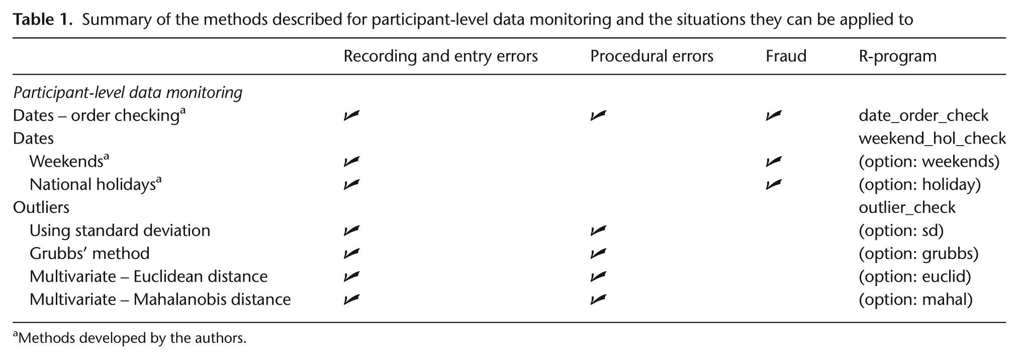
Methods developed by the authors.
Summary of the methods described for centre-level data monitoring and the situations they can be applied to
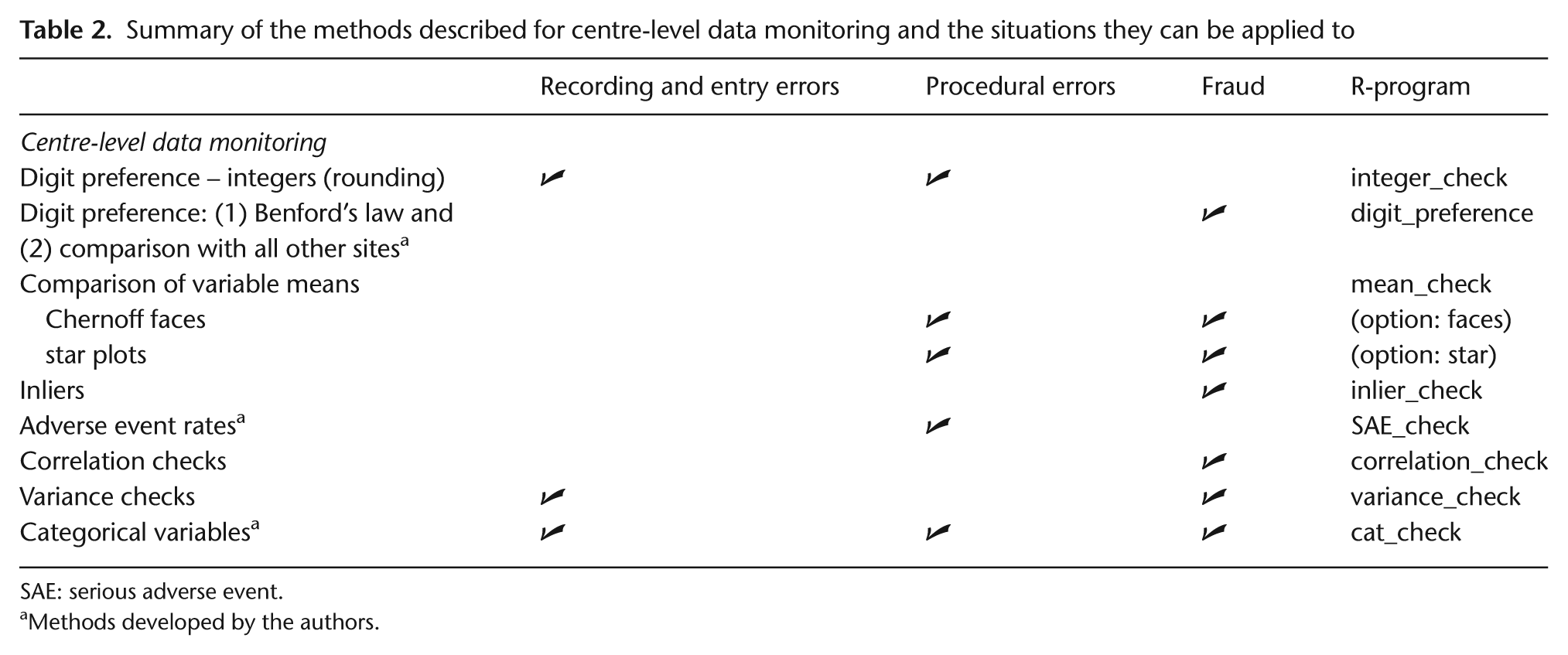
SAE: serious adverse event.
Methods developed by the authors.
Our first goal was to detect data errors at the participant level. Buyse et al. [16] and Baigent et al. [17] suggested calendar checks to find errors such as dates that occur on weekends and holidays (when unexpected) or in an incorrect order, for example, treatment after death. The R-programs to detect outliers, that is, observations that appear too large or too small, were based on univariate (including Grubbs's method) and multivariate approaches (using Euclidean and Mahalanobis distances) [15 –17].
Site (centre)-level data monitoring checks aim to (1) identify systematic errors in trial conduct (procedural errors) at a site, which could be due to a genuine misunderstanding of the trial protocol by local staff, and (2) detect fraud resulting from fabricating trial participants and/or data or creating data for missing values of actual participants [16]. We applied these methods to individual trial sites, but they also could be applied to individual investigators or geographical regions. These checks are intended to flag sites discrepant to the other sites by looking for unusual data patterns, possibly triggering an on-site visit to check the procedures and original data. The methods include examining correlation structures [16 –18] using a method described by Taylor et al. [18], digit preference [15 –17] (including Benford’s law [22]), and inliers [15], that is, participants with several variables whose values lie close to the mean. We also implemented methods to detect procedural errors to identify sites that rounded too many continuous measurements [18] and for repeated continuous measurements, that is, data for a participant with too little variability over time [15,16,20].
Reporting and monitoring adverse events is an important activity in clinical trials. Over-reporting may indicate that site staff are being overly cautious about classifying adverse events, which creates extra work to process reports. However, under-reporting is potentially serious and could affect the trial conclusions as well as regulatory responsibilities. We examined the number of serious adverse events (SAEs) per site based on the number of participants recruited, and the length of time in the trial. We calculated and SAE rate for each site as the number of participants with at least one SAE divided by the total number recruited, and divided further by trial duration at that site. Another method developed used the time each participant spent in the trial.
The methods described above were applied to three phase III cancer trials, in which overall survival was the main end point:
Study 12 [23]: a double-blind trial of 724 patients with small-cell lung cancer, randomised to receive thalidomide or placebo, in addition to standard chemotherapy. Patients were recruited from 79 centres (2003–2006).
ABC-02 [24]: an unblinded trial of 324 patients with advanced biliary tract cancer, comparing gemcitabine/cisplatin with gemcitabine. Here, we also manually created data errors and fabricated patients (one person created them, and another who was blind to the errors ran the R-programs to identify them). Patients were recruited from 37 centres (2002–2008).
TOPICAL [25]: a double-blind trial of 670 patients with non-small cell lung cancer that was ongoing at the time of our assessment of CSM. It compared Tarceva with placebo, among patients considered unfit for chemotherapy. The monitoring findings were checked in real-time with data queries sent to centres. Patients were recruited from 78 centres (2005–2009).
Because Study 12 and ABC-02 had closed already, data could be examined only retrospectively; thus, queries about anomalous or suspicious data were not sent to sites that participated in those trials. We describe how output from the R-programs which apply CSM methods were interpreted. We also provide a summary of their main strengths and limitations in Table 3. We refer to ‘real’ data as those observed from the trials, as opposed to fabricated data that were manually created to evaluate the programs.
Strengths and limitations of the methods

SAE: serious adverse event; CRF: case report form.
Results
Participant-level data monitoring
Dates: ordering, weekends, and national holidays
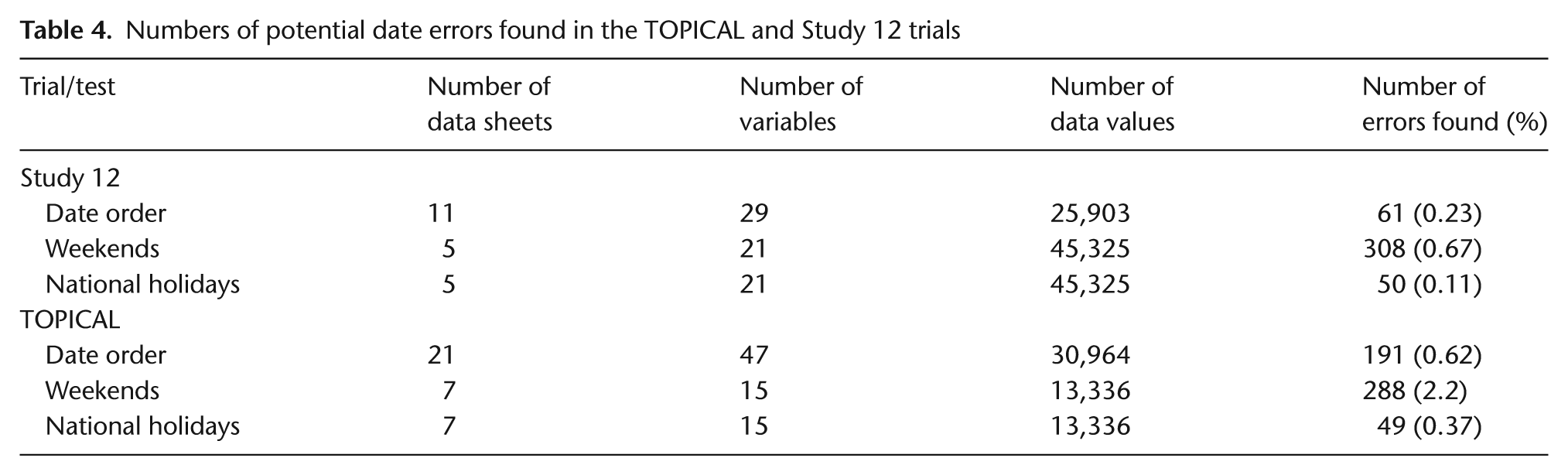
We examined whether dates of randomisation, blood test results, chemotherapy, and follow-up appointments occurred on weekends or holidays and whether there were obvious date ordering errors. The R-program produces tables listing the discrepancies. Very few errors were detected (Table 4) particularly in the Study 12 database, which already had been cleaned and analysed. Weekend and holiday dates from the TOPICAL trial were queried, some were found to be correct (often inpatient treatment), and some were data errors. For Study 12, after inspecting paper case report forms (CRFs) several dates would have been changed. However, there were only 13 living patients for whom any of these dates would be used in survival analyses and corrections would likely have a negligible effect on the results.
Numbers of potential date errors found in the TOPICAL and Study 12 trials
Outliers
Several univariate continuous variables were examined; Figures 1(a) and (b) provide examples of the output (outliers are shown as solid points). The number of data points considered to be outliers using the ±k Standard Deviation (SD) method was 478 (0.93% of all data values) and 148 (1.6%) in Study 12 and TOPICAL respectively. Using Grubbs's test, these numbers increased to 2056 (4%) in Study 12 and 425 (3.3%) in TOPICAL. However, none of these variables were used in the primary analyses.
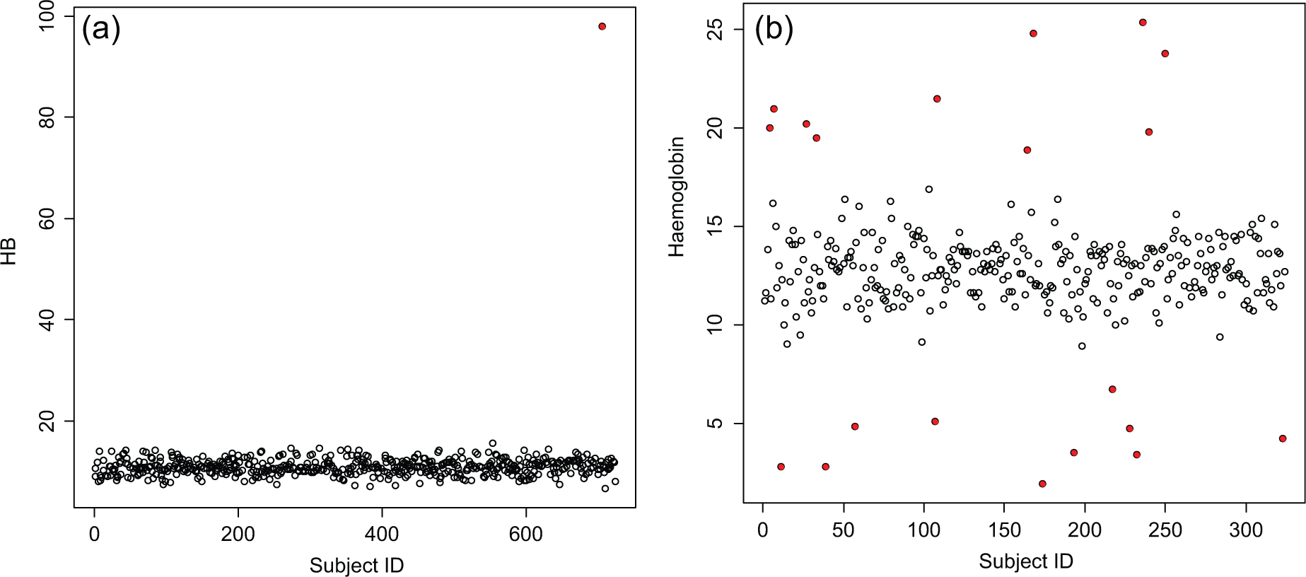
(a) A scatter plot for the Study 12 trial and one continuous variable ‘haemoglobin’ (HB) at baseline. There is only one outlier, automatically shown as a solid point (coloured red in the R output). (b) A scatter plot for the ABC-02 trial and one continuous variable, haemoglobin, at baseline. The points automatically shown as a solid point (coloured red in the R output) are outliers (lying > ±2 SD from the mean). These were all 20 fabricated values that were added to the data set.
Twenty fabricated values were added to the variable ‘haemoglobin’ in the ABC-02 trial by an independent statistician who made them ‘extreme’. The R-program detected 13 out of 20 using a ±3 SD cut-off; the other 7 were found after the 13 had been replaced with their genuine values. All 20 were detected immediately when the cut-off was ±2 SDs (Figure 1(b)) or when Grubbs's test was used at ±3 SDs because the larger false values were removed after each iteration of the program and no longer masked the less extreme outliers. No genuine data values were picked up as outliers with either method. Both methods require the data to be Normally distributed, so our R-programs produce Normal probability plots and histograms. When the data clearly are not distributed Normally, the program could be re-run to detect outliers that lie more than k× inter-quartile range, that is, above and below the upper and lower quartiles.
The R-programs also can be used to check several continuous variables for participants simultaneously (multivariate outliers). We used data from several CRFs for each of the three trials (example in Figure 2). D values, where D is the sum of either the Normalised Euclidean distances or the Mahalanobis distance from the mean (Appendix A), which exceed ±2 SDs from the mean D are automatically shown in red. A list of participants with large D values is also produced. For example, only 13 of 658 patients (2%) using the Euclidean distance and 8 (1.2%) using the Mahalanobis distance were flagged as multivariate outliers in the TOPICAL trial using 19 pretreatment variables simultaneously. A participant identified in both the univariate and multivariate outlier programs could be flagged for particular attention.
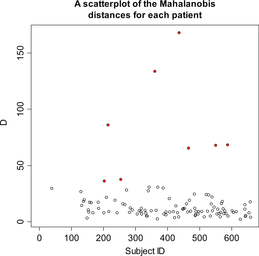
A scatter plot for the TOPICAL trial, based on 19 continuous variables (on the case report form completed at the start of treatment). There are 8 potential multivariate outliers (where D exceeds ±2 SDs), shown in red.
Site-level data monitoring
Rounding and digit preference
The R-program to identify rounding [18] was applied to all of the continuous variables on two CRFs in Study 12. In the example shown in Figure 3, two sites showed a monotonic increase, indicating no evidence of systematic rounding, but site 68 reported only integer values after the first observation.
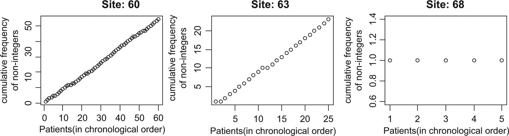
Plot to check for rounding in the variable ‘white blood cell count’ in three different sites in Study 12.
Benford’s law [22] was applied to numeric variables from several CRFs within Study 12 to identify digit preferences. When comparing the observed distribution of leading digits with that expected from Benford’s law, we flagged sites that had p-values ≤0.01 (chi-square test). Table A1 (Appendix A) is the output for Study 12, where 16 out of 65 sites were flagged. However, Benford’s law should be used only for variables where the leading digit can range between 1 and 9, may take values across a range of several orders of magnitude, and are not Normally distributed; assumptions that are unlikely to hold for many clinical trial variables. In Study 12, for example, the data overall did not fit Benford’s distribution (p < 0.001).
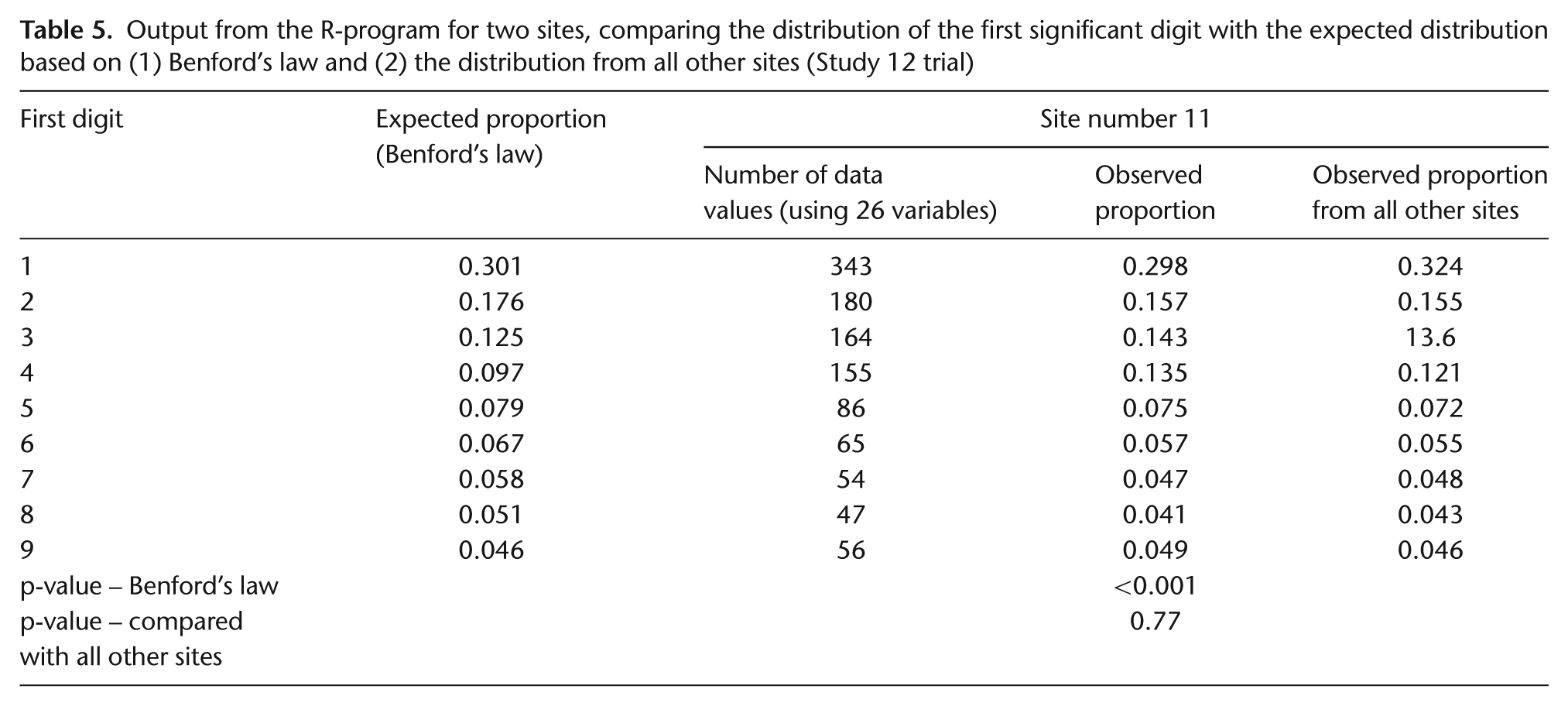
We proposed an alternative method, which compares the observed distribution of leading digits within each site with that from all other sites. This does not have the same limitations as Benford’s law, so all continuous variables could be included (Appendix A–Table A1). For example, the data from site 11 (Table 5) would be flagged using Benford’s law, but when compared with all other sites, its distribution does not appear to be discrepant; indicated by the very different p-values, p < 0.001 versus p = 0.77. The number of sites that were flagged with this method was only 3 of 66 (data from the Study 12 chemotherapy CRF) and 1 of 34 (data from the TOPICAL pretreatment CRF). One site in Study 12 was flagged based on data from the randomisation and chemotherapy CRFs but, on closer inspection, did not appear suspicious because the differences were small and the digit patterns were not similar between the two CRFs. When a large number of data values were examined, even a small difference between the observed and expected proportions sometimes produced a small p-value, so we concluded that the size of the differences should be examined as well as the p-values. Our R-program can also use the last digit of continuous variables instead of the first digit when examining rounding. No sites were flagged using this test on data from either the Study 12 chemotherapy CRF or the TOPICAL pretreatment CRF.
Output from the R-program for two sites, comparing the distribution of the first significant digit with the expected distribution based on (1) Benford’s law and (2) the distribution from all other sites (Study 12 trial)
Comparing means of variables among sites
We implemented three methods for simultaneously comparing the means of continuous measurements among centres: Chernoff face plots [26,27], star plots [27], and parallel coordinate plots (see Appendix A). However, the results from application of these methods were difficult to interpret, and two methods were particularly influenced by outliers. In addition, numerically small differences in the means of variables between one site and another could appear large when displayed as Chernoff faces.
Inliers (data values too close to the means, possibly indicating fraud)
Figure 4 shows a plot used to identify inliers for the TOPICAL trial (based on 19 pretreatment blood values). Similar to the multivariate outlier program, D, the sum of the Euclidean distances from the mean, is calculated for each participant, but here we focus on participants with unusually small D values, which are more apparent on a log scale. Only one patient (from site 20, circled in Figure 4) had a log(Di ) value that exceeded 2.5 SDs below the overall mean log(D)). The number of inliers for the other two trials was also low. Closer inspection of data from patients which were flagged as inliers showed they came from CRFs with small numbers of continuous variables with just one or two of the values lying close or equal to the mean.
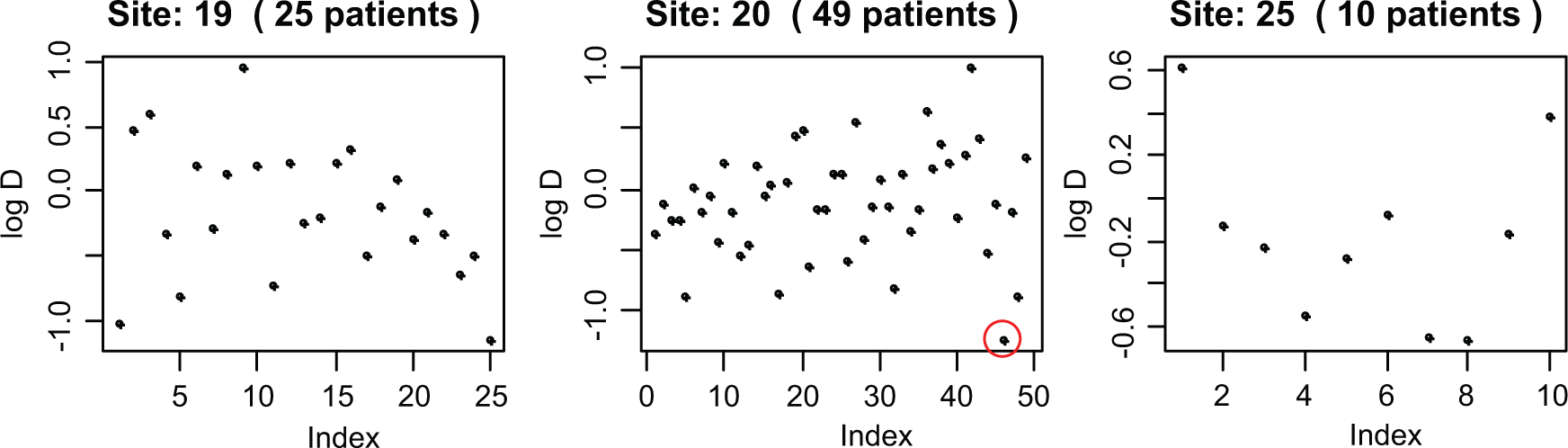
Examining inliers in TOPICAL for 3 sites and 19 variables (i.e., participants who have values too close to the means).
Because few inliers were found in Study 12 and TOPICAL, we fabricated patients in ABC-02 which had data close to the mean values (Appendix A– Text 1, ‘Inliers’). In a site with few patients (n = 9), a cut-off of 2 SDs identified all 6 fabricated patients, and 2.5 SDs flagged four of them. In the site with a medium number of patients (n = 18), no fabricated patients were found using a cut-off of 2.5 SDs, but three were found using 2 SDs. Five fabricated patients in the large site (n = 49) were detected using 2.5 SDs, and all using 2 SDs. However, when several data values are fabricated within a site, they may skew the overall mean and SD of log(D). In this situation fabricated data may not be flagged as inliers, but they may appear to be discrepant on visual examination (Figure 5). Grubbs's test may be helpful for identifying both true inliers and outliers.

Inliers in one site in ABC-02, in which patients (shown as black squares) were manually created to be similar to the means of several variables. In the left-hand figure, there is one fabricated patient automatically flagged (circled) by the program (−2.5 SDs away from the mean D; in the R-program, output appears as a red circle). But in the right-hand figure, there are two fabricated patients. Together they have decreased the variance of d, so they are no longer flagged as inliers (they are not circled in red by the program), but they are apparent on inspection.
Correlation checks
We examined whether a site appeared different from others within the same trial using a set of continuous variables; the output is a grey-scale grid of squares, where each square represents the correlation between two variables. (Colour could be used in place of the grey scale.) Pairs of variables with a correlation coefficient of 1 are indicated by black squares, those with a coefficient of −1 as white squares, and everything else as a shade of grey. Discrepant sites tend to have more light or dark squares than other sites. A formal statistical test using simulations was also applied (see Appendix A– Text 1, ‘Correlation checks’). None of the sites in Study 12 or ABC-02 were flagged, that is, had p < 0.01. In the data from the TOPICAL pretreatment CRF, only two sites had p < 0.01; but on closer inspection, neither site particularly stood out on the grey-scale plots. We concluded that the small p-value may have been influenced by one or two correlations that were weaker or stronger than in the other sites (Appendix A–Figure A1). Both the output display and p-values must be examined when interpreting the results of these checks.
We tested the program by adding fabricated sites using two different methods (Appendix A– Text 1). When sites were created by randomly picking values for each variable from the values seen in other sites, one could create plots that appeared strange, with whole columns that looked strikingly different, but a p-value just above 0.01, particularly in fabricated sites with small numbers of patients (e.g., Figure 6, left panel). When sites were created to have values around the means of each variable, the correlation plots tend to have an overall light grey colour, indicating little correlation. Large fabricated sites (>25 patients) tend to produce a p-value < 0.01. When we ran the R-program 10 times for sites with 30, 35, and 40 fabricated patients, a fake site with p < 0.01 was flagged 19 of 30 times. Close inspection of the output revealed a clear absence of strong correlations that appeared in all other sites (Figure 6, right panel).
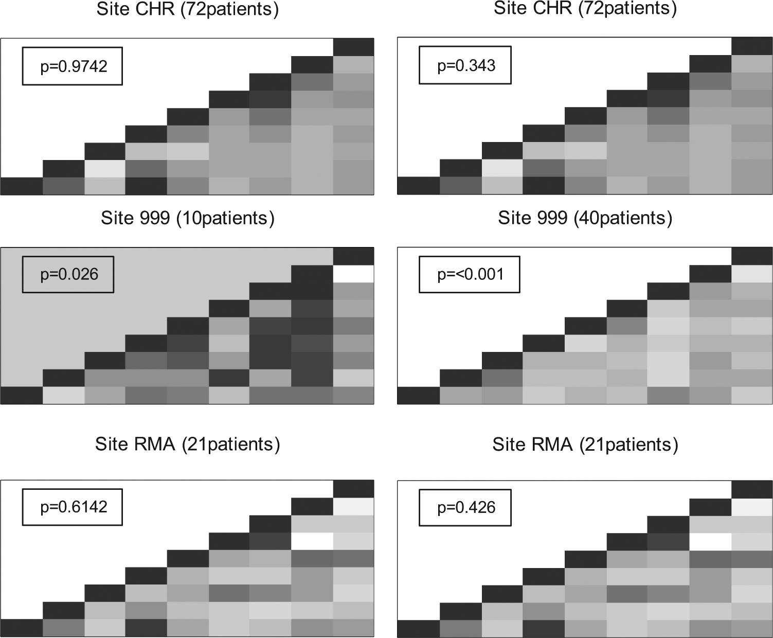
Correlation checks for the ABC-02 trial for 9 variables. Each square represents the correlation between a pair of variables (highly positive = dark colour, highly negative = light colour). Both panels show two real sites (CHR and RMA) and a fabricated site (site 999) generated using randomly chosen values (left panel) or by choosing values close to the mean of each variable (right panel). The p-value for each site is based on simulations which count the number of times a site with a correlation matrix as extreme as that observed could be generated using randomly chosen patients from all other sites.
Variance checks for repeated measures data
Variance checks were made for each of four values from laboratory assays of blood samples taken up to 6 times in Study 12, and 7 such values from up to 18 times in ABC-02. The R-program produced a table showing the percentage of patients in each site which fell into the bottom 2.5% of variances (based on the number of patients checked), and the displays as in Figure 7 (for platelets in ABC-02). In neither trial was a site with patients in the bottom 2.5% of concern. Few sites had more than one outlying patient, often with only a few repeated measurements; and those sites that did had relatively large numbers of patients in total, such that the variances did not appear to be unusual.
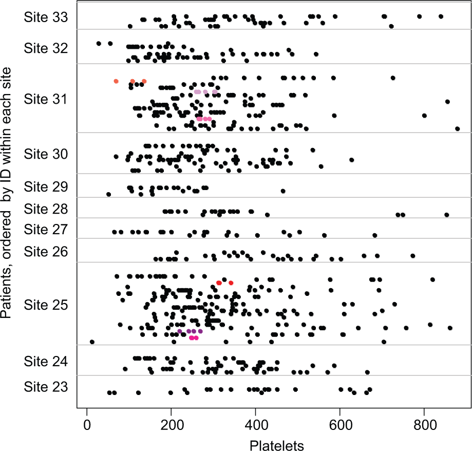
Variance checks for ABC-02. There are three fabricated patients with small variances in site 25 and three in site 31 (shown in shades of red and pink).
In the ABC-02 trial, 11 fabricated patients were added to two sites by an independent statistician; both sites were flagged by the R-program. Seven of the 11 patients had variances in the bottom 2.5% of the distribution for at least 1 of the 7 variables tested, including one fabricated patient who had variances which fell in the bottom 2.5% for 4 different variables. The two sites with fabricated patients appeared in the bottom 2.5% of variances for more variables than any actual trial site. Figure 7 shows the output for sites 23–33; three fabricated patients with low variances are highlighted in sites 25 and 31.
The variance check method involves visual inspection of potentially many displays, with several plots for each variable checked. The number of participants per site, the size of the observed variances, and where the flagged participants fall in relation to others, must be considered when identifying anomalies. For example, several participants with low variance who cluster within a site may indicate fabricated data [20]. Correct transcription of data from CRFs and other measurements for the flagged participants should be checked.
Categorical variables
Categorical variables were checked using chi-square tests which compared each site with all of the remaining sites combined. Two categorical variables were checked in Study 12. For Eastern Cooperative Oncology Group (ECOG) scores and stages, only 5 of 79 and 22 of 79 sites, respectively, had sufficient numbers to be checked. No site had a p<0.01 for ECOG score but 1 did for stage (Table 6). Closer inspection of the observed frequencies revealed no cause for concern. This R-program is particularly useful for large trials with many participants in each site in which the main outcome measure is categorical, for example, response to treatment. Numbers of deaths or disease progressions also could be investigated using this method.
Example of output from the checks of a categorical variable, using the baseline stage in Study 12.
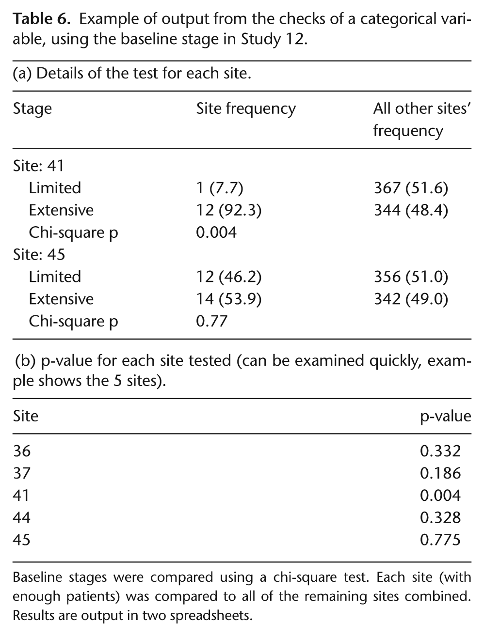
Baseline stages were compared using a chi-square test. Each site (with enough patients) was compared to all of the remaining sites combined. Results are output in two spreadsheets.
Adverse events
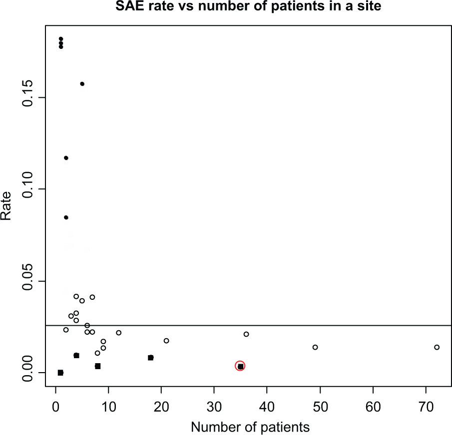
The R-program flags sites that have very few or too many participants with adverse events compared with other sites. We focused on SAEs, but the program could be adapted to examine any type of adverse event. A summary table was produced to show sites from ABC-02 (in which we fabricated data) that are in the lowest and highest 10th centile of SAE rates. The rate was calculated as the number of participants with an SAE in the site divided by the number of participants and the time the site had been recruiting; an example is shown in Tables A2 and A3 (Appendix A). Any centile value can be specified in the R-program. Sites that required further investigation had a reasonable number of participants followed for several months, but had few or no SAEs. We ran simulations by adding a fabricated site to the ABC-02 data 625 times, covering all combinations of numbers of patients (5, 10, 25, 35, or 45), lengths of time in the trial (5, 10, 15, 30, or 45 months), and numbers of patients with SAEs (from 1 to all patients).
Figure 8 is an example of one of the output displays of the rate of SAEs versus the number of participants at each site. The circled black square is the fabricated site (specified as being open for 45 months, having recruited 35 patients but having recorded only 6 SAEs).
Examining SAE rates (ABC-02).
From the simulations, we also attempted to specify the maximum number of SAEs that a site could have but still appear in the bottom 10% of rates (Appendix A–Table A4); for example, in a site with 25 patients which had been open for 30 months, there could be ≤9 patients with an SAE and it would still fall within the bottom 10% of all sites. Such sites, which would fall in the bottom right-hand side of the display in Figure 8 (small SAE rates and relatively large numbers of patients), may warrant further investigation.
The method described above uses an estimated overall time (i.e., time from first randomisation until last randomisation plus ‘x’ months, where ‘x’ is specified as the number of months in which SAEs are expected, i.e. slightly longer than the treatment time. We also used another method of calculating the SAE rate, based on the time spent in the trial by each participant, from date of randomisation through date last seen (Appendix A– Text 1, ‘Adverse events’). Using this approach, the two largest sites were flagged by the R-program because of the long times during which they accrued participants (Appendix A–Figure A2). However, close inspection of the output revealed that their rates were actually larger than the overall rate, although below the median per site, and the total number of SAEs recorded was relatively high, with one site having recorded 65 SAEs for 46 patients and the other 54 SAEs for 32 patients.
Strengths and limitations
The strengths and limitations of each R-program are summarised in Table 3. In most cases, the main limitation to interpretation of output from the programs is the size of the trial. The methods to detect data errors can be applied to all trials; however, many of the methods that aim to detect fraud would be difficult to apply reliably in small trials, or even larger trials when small numbers (<10) of participants are recruited within each site.
Furthermore, the programs that examine possible fraud were created using certain assumptions about the way fabricated data would be generated; when these assumptions are incorrect, that is, a researcher is ‘too good’ at faking data, fraud may not be detected.
Another difficultly is that several methods rely on a visual assessment of output displays, and for these, we added formal statistical tests to aid interpretation. However, the displays should be readily interpreted once the user has gained experience in applying the R-programs, and we stress that the output from no single program should be used as definite evidence of any irregularity at a site.
Finally, we have applied the methods, implemented in the R-programs, only to trials in which fraud was unlikely to have occurred; therefore, we had to fabricate data ourselves to evaluate some methods. We encourage readers to help refine and improve these R-programs by applying the methods to their own databases.
Discussion
We have summarised several methods of CSM by illustrating their application to data from three trials and the main strengths and limitations of each method (Table 3). Although the methods are not perfect, they are easy to implement and interpret. Importantly, they identify certain data errors, such as incorrect dates and outliers, far more quickly and easily than one would during usual data editing and correction processes. They also may help to detect fraudulent sites or participants when fraudulent data are generated in a manner consistent with the assumptions that are the basis of the methods.
The R-programs can be executed automatically and the output should be examined by suitably trained staff. On-site data monitoring visits could be targeted for sites that appear discrepant to the others. During visits to other sites, resources could focus on other on-site activities, such as staff training, helping with accrual, documentation of informed consent, and pharmacy and adverse event checks.
Participant-level data monitoring often is performed during data entry, using automatic validation checks within the database. However, the methods we describe here are not easily programmed into many database systems. Methods such as the correlation check, the inliers, and digit preference program could be applied to as many variables as desired to look for unusual patterns, but we recommend that checks to identify errors and rounding and testing the distributions of categorical data be limited to variables associated directly with safety, treatment compliance, and the primary efficacy end points.
Central site-level monitoring considers both visual assessments of data displays and formal statistical tests. Sites will, by chance, be flagged by one of the methods. Therefore, to avoid too many centres being flagged as suspicious, no single data check should be used automatically trigger an on-site visit. CSM should guide the depth of investigation of anomalies. Consistency of findings from several checks should be used to determine whether a particular centre is identified as suspicious [18]. When we applied the four tests designed to detect potential fraud (digit preference, inliers, correlations, and variance checks) to Study 12, only two sites were flagged by more than one test. Both sites were flagged by the digit preference program and both contained a patient inlier. Further investigation and checks ruled out fraud. More detailed checks also could be performed when a centre is flagged as suspicious before undertaking on-site investigation. For example, if a site reported a particularly low number or rate of SAEs, a first step could be to compare the baseline characteristics of participants enrolled at this site with participants at other sites.
Our R-programs were based on methods suggested by others [15 –18]. Although these articles discussed types of fraud and possible methods of detection, only one applied some of the methods to real data [18]. O’Kelly [28] fabricated participants and a blinded statistician applied methods for inliers, outliers, and unusual correlation structures [18] comparing the results between sites. We agree with O’Kelly who suggested that the actual values of the correlation matrix should be examined, rather than just looking at how different the overall structure is. We did not cover Statistical Process Control (SPC) for clinical trials [29,30]. Most SPC methodology is based on the use of control charts for monitoring a process over time. Similar methods could be used to monitor clinical trials, for example, tracking the average number of SAEs per participant in each trial arm over time.
At present, paper CRFs are used to report data in many trials, including all trials run within our Clinical Trials Unit (CTU) and 57% of Canadian trials [31]. In our vision for the future, a Personal Data Assistant (PDA) would be used for collecting participant data. The PDA would check the data being entered and warn when a possible error was being made or for missing data. At the end of data entry, the forms would be automatically transmitted to the database in the coordinating centre. Participant and centre-level checks, and trial level summaries, would be generated automatically. Trial staff could choose from a menu that allows interactive looks at the data of the types we summarise in our article. For example, for participant-level monitoring, a panel of tables and graphs could appear with demographic details, event dates, missing data, and time plot of when SAEs were recorded. At the site level, there would be a panel showing recruitment graphs, a control chart for SAEs, a control chart for determining the level of on-site monitoring and various fraud test results, and tables and graphs of differences between centres.
In conclusion, CSM can be a cost-effective and worthwhile alternative to on-site source data verification. It can identify anomalous participant data that may be incorrect or fabricated, and sites where the data considered together are quite different from all other sites and therefore should be investigated. The methods are relatively simple to implement and interpret.
Footnotes
Appendix A
To run the R-programs automatically, the variables must appear in a specific order within the data set. To avoid the problem of different trials using different variable names, all of the programs are based on the order in which the variables are given; that is, the participant identification (ID) number must be in the first column and the site name/number in the last (in most cases).
Acknowledgements
Selected for poster presentation at the Annual Meeting of the Society for Clinical Trials (May 2011) and the MRC Clinical Trials Methodology Conference (October 2011). The trial registration details were as follows: Study 14: ISRCTN77341241; TOPICAL: ISRCTN77383050; and ABC-02: ISRCTN82956140.
Funding
This research received no specific grant from any funding agency in the public, commercial, or not-for-profit sectors.
Conflict of interest
None declared.