Sage Journals: Discover world-class research

Abstract

To improve the accuracy of terrain classification during mobile robot operation, an adaptive online terrain classification method based on vibration signals is proposed. First, the time domain and the combined features of the time, frequency, and time–frequency domains in the original vibration signal are extracted. These are adopted as the input of the random forest algorithm to generate classification models with different dimensions. Then, by judging the relationship between the current speed of the mobile robot and its critical speed, the classification model of different dimensions is adaptively selected for online classification. Offline and online experiments are conducted for four different terrains. The experimental results show that the proposed method can effectively avoid the self-vibration interference caused by an increase in the robot’s moving speed and achieve higher terrain classification accuracy.

Keywords

Terrain classification mobile robot RF algorithm feature extraction

Introduction

With the rapid development of mobile robot technology, various mobile robots have replaced humans to complete a broad range of dangerous tasks, for example, search and rescue robots, line-tracking robots, and detection robots. However, these robots are often exposed to the environment, for example, in incidents involving accidents and disasters. Faced with complex working terrains, mobile robots can easily encounter a series of problems such as tire-to-ground sliding, kinematic model changes, and reduced posture reliability. Therefore, to ensure that mobile robots can operate reliably in a variety of complex terrains, experts and scholars have invested in research in the terrain classification abilities of mobile robots.

Currently, mobile robot terrain classification typically uses onboard sensors to identify current or approaching terrain. The interaction between these sensors and the terrain can be divided into two methods: noninteractive and interactive terrain classification. Noninteractive terrain classification methods are mainly implemented by optical sensors (e.g. digital cameras, depth cameras, and laser imaging detection and ranging (LiDARs)).^1,2 The overall accuracy of this method is high but it is easily affected by factors such as light intensity and covering (e.g. branch leaves and turf). The interactive method completes terrain classification through sound and tactile and vibration signals generated by the interaction between the mobile robot and the ground.^3

–6 When considering the external environment, the interactive terrain classification method has better robustness and higher calculation efficiency. Accordingly, this method has significant research potential. Since using sound method uses sound signals to complete terrain classification, it requires installing a microphone on the robot to interact with the external terrain, thereby collecting sound signals to complete the classification. However, due to external noise interference and the inevitable mechanical noise of the mobile robot itself, classification using only sound signals is not ideal.⁷ Terrain classification using tactile signals is mainly used where legged robots are involved and where sensors are installed on the underside of the robot’s foot, enabling it to receive signals that interact with the ground to complete the terrain classification.⁸ Employing vibration signals to complete terrain classification primarily uses the vibration signals generated by the interaction between the ground and the mobile robot tire. The vibration signals change continuously over time and update the z-axis acceleration data intuitively, thereby indicating the terrain features where the robot is located. Compared with sound and tactile signals, vibration signals are better suited for terrain classification involving wheeled mobile robots. Accordingly, the terrain classification method based on vibration signals was adopted for this study.

Significant research is available involving the terrain classification method based on vibration signals. Legnemma et al.⁹ first proposed a terrain classification method based on vibration in 2004. In 2005, Brooks and Iagnemma¹⁰ used power spectral density (PSD) features to extract features of vibration signals based on Legnemma’s ideas. Following dimensionality reduction by principal component analysis (PCA), linear discriminant analysis (LDA) was used to realize terrain classification. In 2012, Brooks and Iagnemma also proposed an unsupervised learning method for terrain classification.¹¹ Without a priori terrain grouping, the vibration signal is fused with the image information to enable the mobile robot to autonomously learn the terrain’s features. Tick et al.¹² proposed a multilevel classifier for terrain classification based on the fusion of acceleration and angular velocity. The acceleration and angular velocity measurement data in three directions are taken, and the linear Bayes algorithm is used for classification after dimensionality reduction. Tick et al. innovatively put forward the idea of using different classifiers at different speeds, with accuracy improving to more than 90%. Xue et al.^13,14 classified terrain using different machine learning classification methods such as support vector machine (SVM) and k-nearest neighbor (KNN) by fusing vibration and acoustic information and extracting time domain features. Xue et al. pointed that the effect of terrain classification using multiple data fusion is better than the effect of using a single type of data. In 2015, Vicente et al.¹⁵ obtained vibration signals via inertial measurement unit (IMU) sensors on a mobile robot equipped with four omnidirectional wheels and completed feature extraction in the time and frequency domains. The PCA algorithm was used to reduce the dimensionality. The extreme learning machine algorithm completed the classification of four different floors (e.g. carpet, wooden floor, and so on) at an accuracy rate exceeding 85%. In 2017, Zhao et al.^16,17 set up sensors on the suspension and seats of a car to collect vibration data and extracted features in the time, frequency, and time–frequency domains. They used the relief algorithm to evaluate the importance of features and to reduce dimensionality and, finally, used a voting algorithm to determine the type of terrain. In 2019, Mei et al.¹⁸ performed a terrain classification method study on wheeled robots with shock absorbers; their results indicated that vibration signals would be significantly weakened on such robots, thus affecting the accuracy of traditional terrain classification methods. Then, a long–short-term memory network based on one-dimensional convolution was proposed as a terrain classification method. Bai et al.¹⁹ proposed a terrain classification method based on multilayer perceptual deep neural networks, which has significantly improved accuracy compared with traditional backpropagation neural network classification. Concurrently, they also proposed that in different terrains, different robot speeds will affect the accuracy of terrain classification. In the same year, other scholars proposed terrain classification methods that combined vibration signals with other signal types (not repeated here).^20,21

Based on existing research, this article pays more attention to the influence of mobile robot speed on terrain classification accuracy (ACC). The main novel contributions of this article are summarized as follows: (1) consider the impact of robot speed on the accuracy of terrain classification, (2) refine the attributes of the classifier and generate a full feature model and a partial feature model according to the different types of extracted features, and (3) the concept of critical speed is proposed, and different characteristic models are used based on the relationship between the current speed of the mobile robot and the critical speed.

Adaptive online terrain classification algorithm

In this study, a differential four-wheel mobile robot moved at a constant speed on hard ground, grassland, small- and large-gravel terrain, respectively, and obtained acceleration signals comprising vibration information from an IMU installed on top of the robot. The interaction between the tire and the ground generated a vibration signal, which changed the magnitude of the acceleration signal in real time. Since it is assumed that the robot is moving on a plane, the z-axis acceleration direction can be considered to be always perpendicular to the ground, which is used to reflect the characteristic information of different terrains.

The entire terrain classification algorithm was divided into two stages: offline training and online classification. In the offline training phase, the z-axis acceleration signal was first divided into data segments at equal distances. Each data segment included data of the mobile robot moving at a constant speed for 1.5 s. When the speed of the mobile robot was lower than the critical speed, the time domain characteristic values of the acceleration signal was extracted. When it was higher than the critical speed, based on extracting the characteristic values of the acceleration signal in the time domain and then extracting the characteristic values in the frequency and the time–frequency domains, the feature vector was obtained after the end-to-end connection. The terrain labels were all marked at the end of the data line. When the operating speed of the mobile robot was lower than the critical speed, the feature vectors were input to the random forest (RF) classifier to generate the partial feature model; when it was higher than the critical speed, the feature vectors were input to the RF classifier to generate the full feature model. The generated full feature model and partial feature model can be used directly in the online classification stage. In the online classification phase, first, different classifier models were selected according to the relationship between the robot’s current speed and the critical speed. Then, the same data preprocessing was performed as in the offline training phase on the newly acquired data, and the results were entered into the corresponding classifier model to obtain the terrain type of the robot. The overall flowchart of the algorithm is shown in Figure 1.

Figure 1.

Algorithm overall flowchart.

Feature extraction

This article proposes a feature extraction method based on extracting a different number of features in the time, frequency, and time–frequency domains at different speeds. When the speed of the mobile robot was lower than the critical speed, only the time domain features were extracted. When it was higher than the critical speed, based on time domain features, PSD and discrete wavelet transform (DWT) were used to extract the frequency and time–frequency domain features. PSD is a physical quantity that characterizes the relationship between signal power energy and frequency, and it is often used to study random vibration signals. DWT is to discretize the scale and translation of the basic wavelet. DWT examines the frequency domain characteristics of the entire time domain process or the time domain characteristics of the entire frequency domain process.

To eliminate the average value component in the acceleration data obtained, first, each group of data was zero-averaged. Then, the average amplitude, square root amplitude, absolute maximum value, minimum value, peak-to-peak value, local maximum value, mean square value, root mean square value, peak factor, maximum deviation, and kurtosis in each data segment were calculated as the time domain characteristic values (11 characteristic values in total).¹³ A 1024-point fast Fourier transformation is used to extract the PSD feature in each data segment. However, it should be noted that only the magnitudes are kept while the corresponding phases are ignored. To improve computation efficiency and to maximize the classification performance, only the majority of components that carry most of the useful information are retained. Namely, the first 256 components are selected.²² In the time–frequency domain, DWT is used to extract the features of the data segment. Select “Daubechies 4 (db4)” as the internal mode of the DWT function and can get 106 eigenvalues of each data segment.¹⁶ Using Daubechies wavelet can make the signal reconstruction process smoother. When the operating speed of the mobile robot is higher than the critical speed, the three types of characteristic values extracted from the time domain, frequency domain, and time–frequency domain are connected through the “append” function of python. Finally, each data segment generated 373 feature vectors. In the offline training phase, after extracting features from all the data segments, an n-dimensional feature vector matrix was generated. Then, the feature vectors of each column were normalized according to the following formula

X_{i} = \frac{X_{i} - X_{mean}}{std}

where X_i is the ith characteristic value, $X_{mean}$ is the average of the characteristic values, and $std$ is the standard deviation of the characteristic values. After normalization, all characteristic values were clustered around 0 and the variance was 1.

The random forest online classification algorithm principle

The RF algorithm is an extension of the Bagging algorithm. When creating Bagging integration using unpruned decision trees, RF adds random attribute selection in the training process of decision trees and finally generates classification results by voting of all decision trees.

The RF algorithm can be applied in the context of classification and regression. If a decision tree is regarded as an expert approach in classification tasks, then RF is the classification of specific tasks by multiple experts. The steps for generating RF are as follows:

1. The bootstrapping method is used to randomly draw samples m times from a given set containing M samples. After each sampling, the sample is returned to the data set. The collected data is then put into the training set. The probability of a sample not appearing after m samplings can be obtained from the following formula

lim_{x \to \infty} {(1 - \frac{1}{m})}^{m} = \frac{1}{e} \approx 0.368 (2)

A total of n sampling operations were performed to generate n training sets.

2. For n training sets, n training tree models were generated by training. For each node of a single decision tree, first, a subset containing k attributes was selected from the attribute set. Generally, in $k = {log}_{2} d$ , d is the number of attribute sets. The trees in the random forest algorithm can be processed using ID3, C4.5, and classification and regression tree (CART) algorithms. Compared with ID3 and C4.5 algorithms, the CART algorithm can use the training set and cross-validation set to continuously evaluate the performance of the decision tree to prune the decision tree, so that the training error and the test error can reach a good balance. Therefore, the CART algorithm is used as the internal processing algorithm of the random forest algorithm. In the CART algorithm, the attribute with the smallest Gini index is selected as the split attribute of the root node of the decision tree. The Gini index calculation can be obtained using the following formula

Gini (s) = 1 - \sum_{i = 1}^{k} p_{i}^{2} (3)

where s represents the current training set and p_i is the probability that data with a specific attribute will be present in the training set. The decision trees are not pruned to maximize their splitting until all the data of the node belongs to the same class.

3. The generated multiple decision trees form an RF that classified the newly input data according to formula 4, while the tree classifiers’ voting results determined the final classification

H (x) = \underset{Y}{arg
max} \sum_{i = 1}^{n} I (h_{i} (x) = Y)

where $h_{i} (x)$ is the classification result of a single decision tree, Y is the target classification, $I (\cdot)$ is the illustrative function, n is the number of decision trees, argmax is the maximum independent variable point set of the function, and $H (x)$ is the final classification result. The RF online classification algorithm flowchart is shown in Figure 2.

Figure 2.

The RF online classification algorithm flowchart. RF: random forest.

In the system presented herein, following feature extraction, the original vibration signal generated a data set including m samples. The core of the RF is its two randomnesses, including random data extraction and random feature extraction. First, it randomly extracts data m times from the data set to generate a training set; then, according to $k = {log}_{2} d$ , an attribute set containing k attributes is extracted. These k attributes are then used to train the data set to generate a tree. The entire process is repeated n times to generate a trained RF including n numbers. Then, the original vibration signal to be classified is input into the RF after feature extraction and the terrain classification result is obtained. The overall framework of the RF algorithm in the system is shown in Figure 3.

Figure 3.

The overall framework of the RF algorithm in the system. RF: random forest.

Experimental design and results

Experimental method

The mobile robot terrain classification system included a four-wheeled side-sliding mobile robot, an IMU, and a host computer. This article is based on the Robot Operating System (ROS, v.ROS Kinetic Kame) software framework, run under the Ubuntu system (Ubuntu, v.16.04) to complete the data collection and experimental work. A four-wheeled side-sliding mobile robot was used as the experimental platform, and the IMU and host computer were installed on top of the robot. The mobile robot experiment system is shown in Figure 4. The four-wheeled side-sliding mobile robot weighed 65 kg and its entire body was symmetrical. The body comprised a metal structure without a suspension system. The four tires of the mobile robot were made of solid rubber. The host computer used an Intel NUC8i7BEH with a Core i7-8559U processor and 16 GB memory. The IMU selected Xsens MTI-300-2A8G4 with a frequency of 100HZ. The two-dimensional LiDAR used the LMS1xx series of products produced by SICK, with a measurement range of up to 50 m and a scanning angle of $270^{\circ}$ in the horizontal plane. The two-dimensional lidar is centrally installed in front of the robot, about 40 cm from the ground. As the robot traversed different terrain types, the integrated three-axis direction accelerometer of the IMU sensed changes in vibration signals and returned real-time acceleration data. Only need to subscribe to the topic of the accelerometer of ROS under the terminal to complete the data collection.

Figure 4.

The mobile robot experiment system.

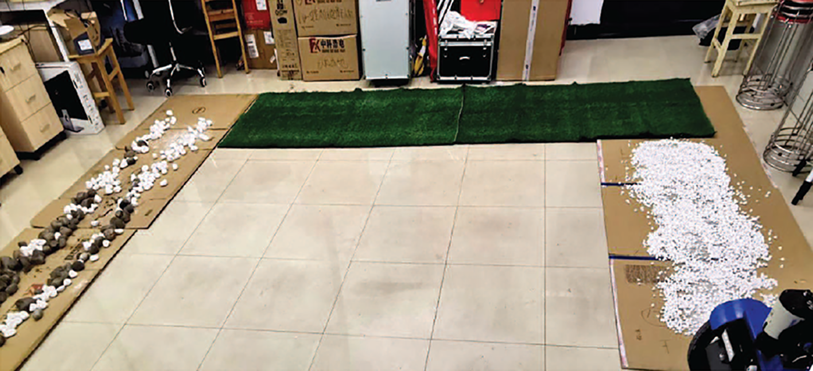
The experimental terrain was divided into four types: hard ground (the ground was flat and hard without potholes), grassland (artificial grass, grass length 2–3 cm), a small-gravel road (diameter of gravel 1–1.5 cm), and a large-gravel road (diameter of gravel 3–5 cm). The pavement was artificially laid and was 2 m long and 1 m wide. The experimental terrain is shown in Figure 5. During the experiment, the tires were in full contact with the terrain. Related experiments on the gravel road ensured the even distribution of the gravel. The sliding robot moved at five speeds of 0.1, 0.2, 0.3, 0.4, and 0.5 m/s, respectively, and traveled uniformly on the four surfaces to obtain acceleration data.

Figure 5.

Experimental terrain.

Figure 6 shows the mobile robot’s z-axis acceleration data that collected when the mobile robot moved at 0.1 m/s on each of the four terrains. The x-axis represents time (s) and the y-axis is acceleration (Acce/ $(m / s^{2})$ ). The peak-to-peak value of the hard ground and the grassland was similar because the artificial grass used in the experiment included hard ground underneath it. However, because the grass was uneven, the vibration frequency obtained by the robot on the grass was significantly higher compared with the hard ground. The peak-to-peak values of the small- and large-gravel roads were significantly higher than those on hard ground and grassland. This was because of the collision that occurred between the robot and the gravel; the faster the robot moved, the greater the kinetic energy generated by the collision and the higher the peak. The vibration frequency depended on the gravel density and the speed of the robot. Therefore, compared with the other three types of terrain, the distribution density of gravel of large-gravel road is lower, and the frequency of the obtained vibration signal is correspondingly lower.

Figure 6.

Acceleration data at the same speed and on different terrains.

As the speed of the mobile robot increased, the vibration and noise caused by the vehicle body also affected the acceleration data. Figure 7 shows the mobile robot’s z-axis acceleration data corresponding to different speeds when the mobile robot moved on hard ground. The x-axis represents time (s) and the y-axis acceleration (Acce/ $(m / s^{2})$ ). It is shown that when the mobile robot moved at a low speed, the acceleration data were stably maintained near 9.8/ $(m / s^{2})$ . The classified model that needs to be trained is relatively simple when the robot operates at this time. However, as the vehicle speed increased, the peak-to-peak value and vibration frequency of the obtained z-axis acceleration data increased significantly. It is easy to confuse the hard ground with the other three types of uneven terrain. Therefore, more complex training models are required to improve ACC. It can be further hypothesized that if the same model classifier is used at various speeds, the ACC will be affected. Furthermore, this will be improved the case if critical speed is adopted to adaptively change the choice of classifier model during online classification. When the mobile robot’s current speed was lower than the critical speed, the partial feature model was adopted. When the current speed was higher than the critical speed, the full feature model was used. In this manner, ACC can effectively be improved.

Figure 7.

Acceleration data at different speeds on the same terrain.

Experimental evaluation criteria

In this article, the result of the 10-fold cross-validation and confusion matrix was primarily used as the evaluation criteria for the experimental results.

Cross-validation is a statistical analysis method used to verify the performance of a classifier. Also known as cyclic estimation, it is a practical method for statistically cutting data samples into small subsets. Ten-fold cross-validation evenly divided the original data into 10 groups. For each test, nine groups of data were used as the training set and one group of data was used as the test set. Each group of data was tested once, and a total of 10 models were yielded. The average ACC among the 10-model test set was then derived as the performance index of the classifier under 10-fold cross-validation.

The confusion matrix is a standard format for expressing accuracy evaluation and serves as a visualization tool particularly suited to supervised learning. The confusion matrix can display the accuracy of the classification results in a matrix that is primarily used to compare the classification results with the actual measured values. A two-class confusion matrix is shown in Table 1.

Table 1.

Binary classification confusion matrix.

		Predicted condition
		Predicted condition positive	Predicted condition negative
True condition	Condition positive	True positive (TP)	False negative (FN)
True condition	Condition negative	False positive (FP)	True negative (TN)

Each column of the confusion matrix represents the predicted category, and the total number of each column represents the degree of data predicted to be included in the said category; each row represents the true category of the data, and the total data of each row represents the level of data of that category. The ACC obtained from the confusion matrix is expressed by the following formula

ACC= \frac{TP+TN}{TP+FN+FP+TN}

Selection of the feature model and algorithm

In the experiments in this section, for each terrain, 150 time-continuous samples were taken at the same speed as for a set of data. For each terrain, 40 data sets were obtained for each specific speed. Six single algorithms were selected: logistic regression, LDA, KNN, CART, naive Bayes classifier (NB), and SVM. Furthermore, four integrated algorithms, bagging decision tree (BDT), RF, extreme random tree, and adaptive boosting (AB) were also included. The result of 10-fold cross-validation was selected as the evaluation criterion for the ACC of the algorithms. The experiments in this section did not adjust the internal parameters of any of the algorithms.

As noted above, when the mobile robot’s motion speed increased, the vibration of the vehicle body will be mixed into the vibration signal as noise, causing the complexity of the classification model to increase. Therefore, it is necessary to adaptively select feature models of different complexity based on the different moving speeds of the mobile robot. The accuracy of each classification algorithm under different features and at five different speeds of a mobile robot is shown in Figure 8.

Figure 8.

Comparison of the accuracy of classification algorithms under different speeds and different features. (a) Comparison of the accuracy of classification algorithms with different features at 0.1 m/s. (b) Comparison of the accuracy of classification algorithms with different features at 0.2 m/s. (c) Comparison of the accuracy of classification algorithms with different features at 0.3 m/s. (d) Comparison of the accuracy of classification algorithms with different features at 0.4 m/s. (e) Comparison of the accuracy of classification algorithms with different features at 0.5 m/s.

Based on the comparison charts, regardless of the specific classification algorithm used, the classification effect obtained by the time domain and merged features (time, frequency, and time–frequency domain fusion) were the best. Therefore, time domain features were selected as the partial feature model, and fusion features were selected as the full feature model.

The following compares and evaluates the accuracy of a single and an integrated algorithm. The experiment used data collected at 0.3 m/s by a mobile robot as a data source and employed the full and partial feature model to compare the accuracy of the classification algorithm. A comparative box plot is shown in Figure 9.

Figure 9.

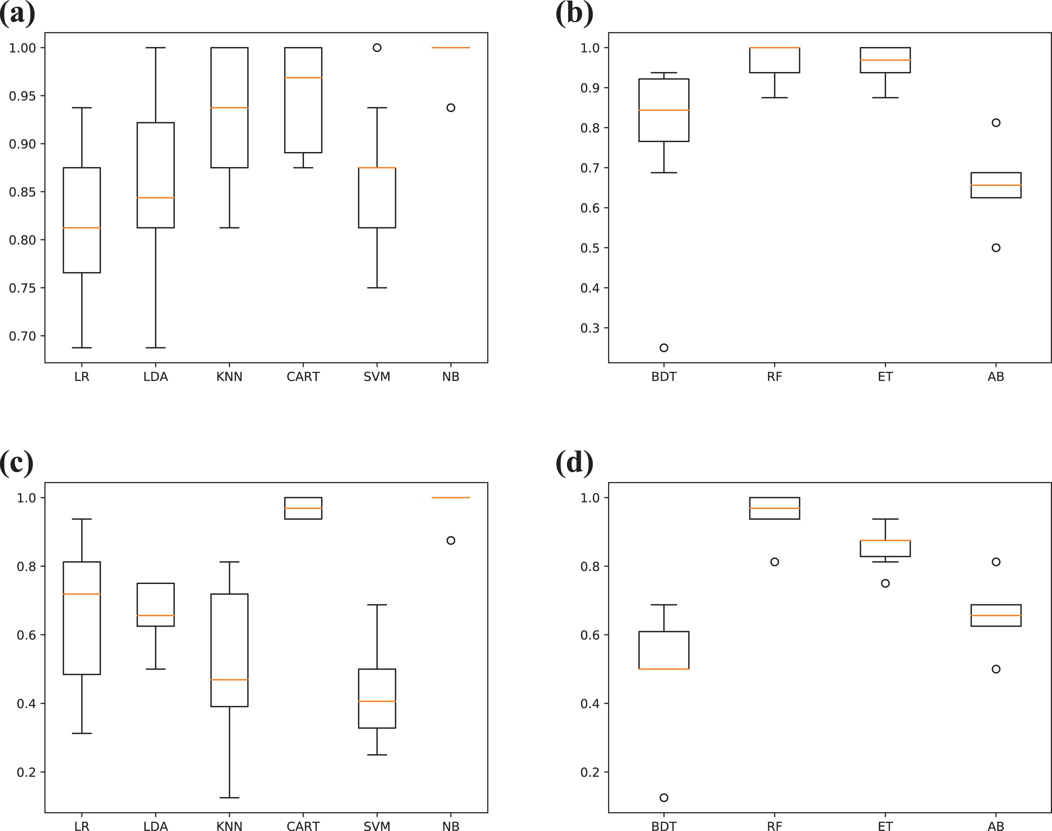
A box plot indicating the accuracy of each classification algorithm under different feature models at 0.3 m/s. (a) Single algorithm comparison box plot (partial feature model). (b) Integrated algorithm comparison box plot (partial feature model). (c) Single algorithm comparison box plot (full feature model). (d) Integrated algorithm comparison box plot (full feature model).

It is shown that, for the single algorithm, the CART algorithm performed best, where the precision median line was higher and the distribution was the most uniform. The NB algorithm exhibited an obvious overfitting phenomenon. In the integrated algorithm, in addition to the AB algorithm, the accuracy of the remaining integrated algorithms under the two feature models had improved significantly compared with the accuracy of the single algorithm, and the median line of the accuracy of the RF algorithm was above 80%. According to a series of comparative experiments, the RF algorithm showed the best classification performance and will thus be used as a classifier for the adaptive online terrain classification algorithm.

Selection of critical speed

The system developed in this article used two training classification models of different complexity based on the speed of the mobile robot. By judging the relationship between the current vehicle speed and the critical speed, the selection of the model was adaptively completed. At five speeds, 40 sets of samples were taken from each terrain. Finally, a data set including 160 sets of data was generated at each speed. Using the full feature and partial feature models, the average ACC of the two models at different speeds was obtained through 10-fold cross-validation. The comparison chart for the ACC model at different speeds is shown in Figure 10.

Figure 10.

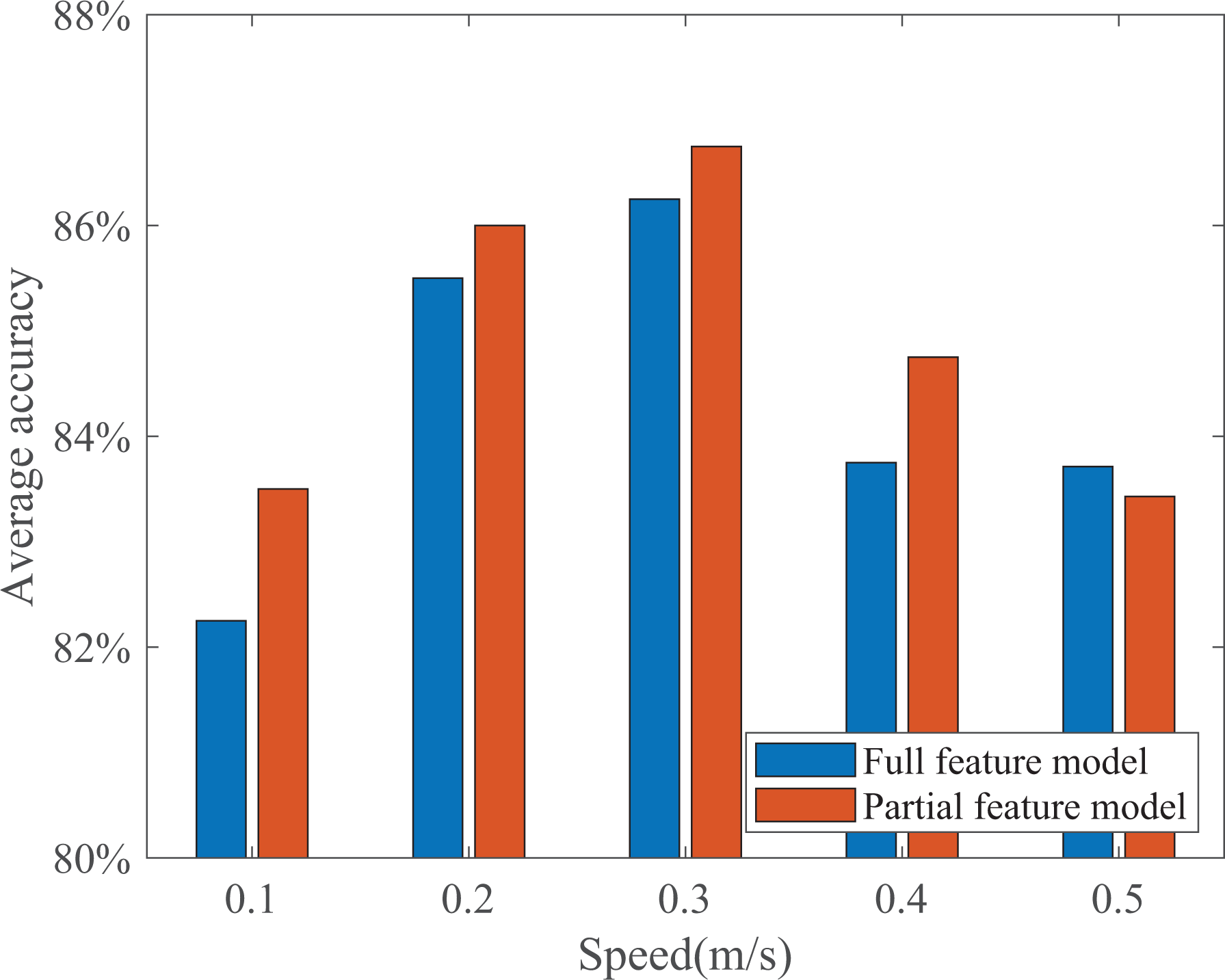
Comparison of the ACC model at different speeds. ACC: terrain classification accuracy.

The figure shows that for 0.1–0.4 m/s, the ACC obtained using the partial feature model was slightly higher compared with the full feature model. At 0.5 m/s, the ACC obtained using the full feature model was higher. Therefore, it was necessary to choose a value of appropriate size as the critical speed. The critical speed is defined as a running speed of the robot. When the critical speed is less than or equal to the critical speed, the system adopts a partial characteristic model, and when the critical speed is higher than the critical speed, the full characteristic model is used. In this experiment, 0.4 m/s is selected as the critical speed of the mobile robot.

3.5 Adaptive terrain classification algorithm accuracy

Experiments were performed at different speeds using adaptive terrain classification algorithms. The original data set was divided into training and test training sets, which accounted for 67% and 33% of the total data, respectively. The classification results are presented in Table 2, where V represents speed and AAC represents average ACC.

Table 2.

Classification results of four terrains at five speeds.

V = 0.1 m/s		Predict terrain
AAC: 90.57%		Hard ground	Grassland	Small-gravel road	Large-gravel road
Actual terrain	Hard ground	93.3%	0.07%
	Grassland	33.3%	66.7%
	Small-gravel road			100%
	Large-gravel road				100%
V = 0.2 m/s		Predict terrain
AAC: 94.34%		Hard ground	Grassland	Small-gravel road	Large-gravel road
Actual terrain	Hard ground	86.67%	13.33%
	Grassland		100%
	Small-gravel road			100%
	Large-gravel road			7.69%	92.31%
V = 0.3 m/s		Predict terrain
AAC: 96.23%		Hard ground	Grassland	Small-gravel road	Large-gravel road
Actual terrain	Hard ground	93.75%	6.25%
	Grassland		100%
	Small-gravel road	7.69%		92.31%
	Large-gravel road				100%
V = 0.4 m/s		Predict terrain
AAC: 92.45%		Hard ground	Grassland	Small-gravel road	Large-gravel road
Actual terrain	Hard ground	92.31%	7.69%
	Grassland	23.08%	76.92%
	Small-gravel road			100%
	Large-gravel road				100%
V = 0.5 m/s		Predict terrain
AAC: 91.49%		Hard ground	Grassland	Small-gravel road	Large-gravel road
Actual terrain	Hard ground	84.62%	15.38%
	Grassland		100%
	Small-gravel road			100%
	Large-gravel road			28.57%	71.43%

The table shows that the accuracy rate of the adaptive terrain classification algorithm was higher than 90%. With an increase in speed, the accuracy reached 96.23% at 0.3 m/s. This happened because as the speed increased, the collision between the wheel and the ground became more intense, and the vibration signal data reflected by the acceleration was clearer and more effective. However, as the speed increased further, the noise caused by the vibration of the robot body became more intense. Although the full feature model had been used at this time, the accuracy rate still inevitably decreased. Table 2 also shows that the hard ground and grass terrains could easily be confused. At 0.1 m/s, nearly one-third of the grassland data segments were considered as being hard ground. This happened because the grass itself was relatively soft; as such, the mobile robot did not easily vibrate on the grassland, which had hard ground underneath it. The small -and large-gravel terrain classifications had higher accuracy.

To show that the accuracy of the adaptive terrain classification algorithm had been improved compared with previous terrain classification algorithms, the accuracy of terrain classification using RF algorithms based on three different classification models at different speeds was compared. The accuracy comparison line chart is shown in Figure 11. Among the classifications, RF-AUTO represents an adaptive terrain classification algorithm, RF-PART is an RF algorithm that extracted the partial feature model for classification, and RF-ALL represents an RF algorithm that extracted the full feature model for classification. It can be seen that the overall accuracy of the adaptive terrain classification algorithm was higher than the accuracy of the RF algorithm using the full feature model or the partial feature model only.

Figure 11.

Comparison chart of RF algorithm accuracy under different models. RF: random forest.

Online experiment

To verify the accuracy of the online classification of the algorithm in practical application scenarios, a mobile robot was driven on four different terrains that were prepaved to gain real-time terrain classification results. Since the mobile robot would adaptively switch models at different speeds, when designing the experiment, we considered changing the speed of the mobile robot when moving on the same terrain to ensure that all the different robot speeds were reflected during the experiment. The experimental scene is shown in Figure 12.

Figure 12.

Experimental results of the online adaptive terrain classification algorithm.

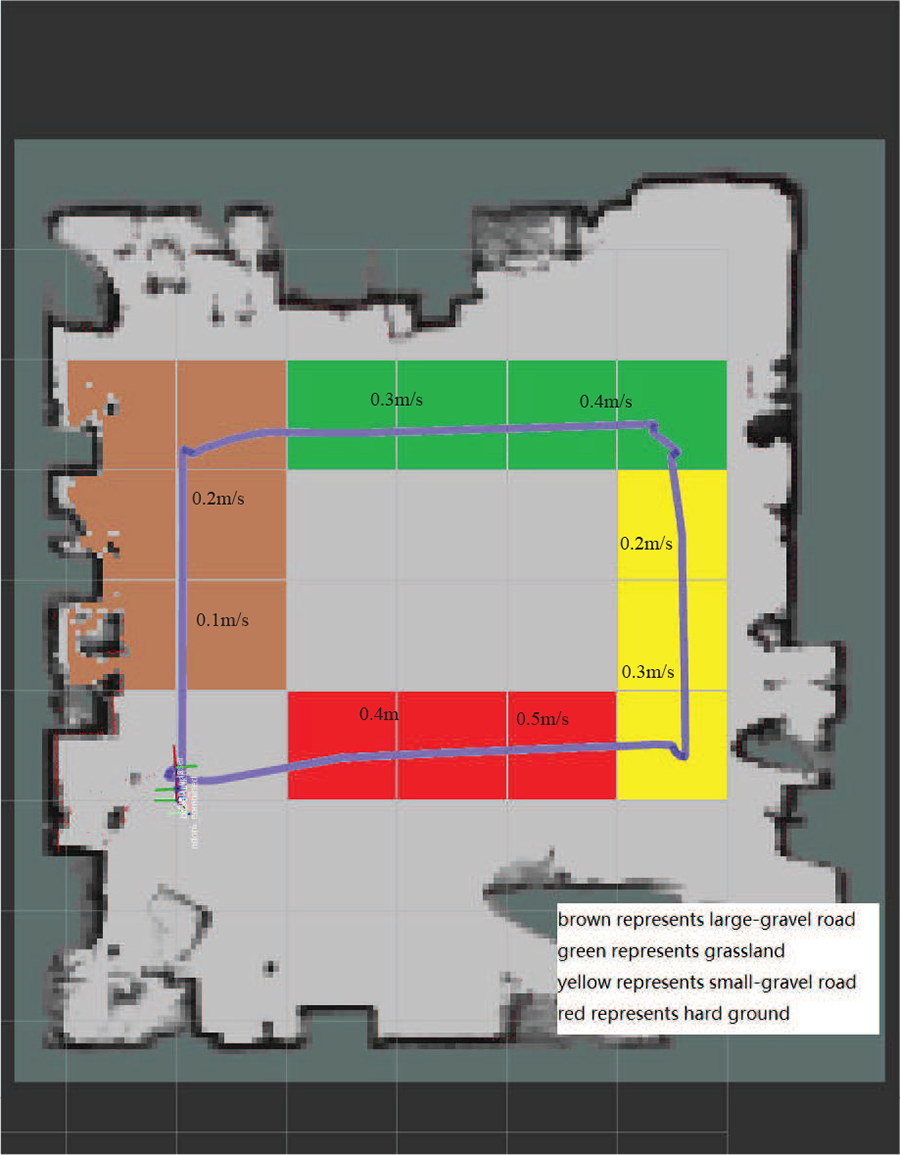
Select some positions in advance as the nodes for speed switching. When the mobile robot moves to the specified position, its moving speed can be changed instantaneously by the remote control. The trajectory of the entire moving process was an approximately 4 m $\times$ 3 m rectangle, that is, the purple trajectory zone in Figure 13. The various terrains that the mobile robot traversed in the experiment are represented by different colors in the image: brown represents the large-gravel road, green represents the grassland, yellow represents the small-gravel road, and red represents the hard ground.

Figure 13.

Robot movement path.

Ignoring the start and end times of the mobile robot, the entire experimental process time was 57 s. The average time for the system to perform terrain classification was approximately 0.3 s, and 34 classification data points were obtained. This was sufficient for meeting the requirements of online classification. The results of online experiments are shown in Figure 14. The blue line represents the ideal terrain classification result and the red line represents the experimental terrain classification result. The overall accuracy of the classification was 94.12%.

Figure 14.

Experimental results of the online adaptive terrain classification algorithm.

Conclusion

This article proposed an adaptive online terrain classification method based on vibration signals. Compared with the use of a single model for terrain classification in existing terrain classification research, it effectively improved ACC and placed a more significant focus on the impact of speed changes on the accuracy of a mobile robot’s terrain classification.

First, through a series of comparative experiments, the time domain and merged features of the time, frequency, and time–frequency domains were determined as the training features of the partial feature model and the full feature model, and the RF algorithm was determined as the classifier. Then, this article proposed a method for adaptively selecting models of different complexity for training and classification, based on the magnitude relationship between the mobile robot’s speed and its critical speed. Through a subsequent comparative test, the critical speed of the mobile robot was determined. Finally, the effectiveness of the method was proven by offline and online experiments. Based on a series of tests, the accuracy of the classification results obtained using the adaptive terrain classification method was higher than 90%.

We found that selected classification algorithms had excellent ACC when targeting certain features. Therefore, in follow-up research, we aim to further investigate methods of terrain classification using two or more different algorithms simultaneously.

Footnotes

Declaration of conflicting interests

The author(s) declared no potential conflicts of interest with respect to the research, authorship, and/or publication of this article.

Funding

The author(s) disclosed receipt of the following financial support for the research, authorship, and/or publication of this article: This work was supported by the National Natural Science Foundation of China under Grant No. 51674169 and the Department of Education of the Hebei Province of China under Grant Nos. ZD2018039 and No. ZD2017069.

ORCID iD

Liming Ye

References

Vandapel

Huber

Kapuria

, et al. Natural terrain classification using 3-d ladar data. In: IEEE international conference on robotics and automation (ICRA), New Orleans, LA, 26 April–1 May 2004, pp. 5117–5122. IEEE.

Narváez

Gregorio

Escolà

, et al. Terrain classification using ToF sensors for the enhancement of agricultural machinery traversability. J Terramech 2018; 76: 1–13.

Christie

Kottege

. Acoustics based terrain classification for legged robots. In: IEEE international conference on robotics and automation (ICRA), Stockholm, Sweden, 16–21 May 2016, pp. 3596–3603. IEEE.

Valada

Burgard

. Deep spatiotemporal models for robust proprioceptive terrain classification. Int J Robot Res 2017; 36: 1521–1539.

Huh

Mukherjee

, et al. Integrated ground reaction force sensing and terrain classification for small legged robots. IEEE Robot Automat Lett 2016; 1: 1125–1132.

Walas

Systems

. Terrain classification and negotiation with a walking robot. J Intellig Robot Syst 2015; 78: 401–423.

Libby

Stentz

. Using sound to classify vehicle-terrain interactions in outdoor environments. In: IEEE international conference on robotics and automation (ICRA), Saint Paul, MN, 14–18 May 2012, pp. 3559–3566. IEEE.

Hoepflinger

Remy

Hutter

, et al. Haptic terrain classification for legged robots. In: IEEE international conference on robotics and automation (ICRA), Anchorage, AK, 3–7 May 2010, pp. 2828–2833. IEEE.

Legnemma

Brooks

Dubowsky

. Visual, tactile, and vibration-based terrain analysis for planetary rovers. In: IEEE aerospace conference proceedings (IEEE Cat No 04TH8720), Big Sky, MT, USA, 6–13 March 2004, pp. 841–848. IEEE.

10.

Brooks

C A

Iagnemma

. Vibration-based terrain classification for planetary exploration rovers. IEEE Trans Robot 2005; 21: 1185–1191.

11.

Brooks

C A

Iagnemma

. Self-supervised terrain classification for planetary surface exploration rovers. J Field Robot 2012; 29: 445–468.

12.

Tick

Rahman

Busso

, et al. Indoor robotic terrain classification via angular velocity based hierarchical classifier selection. In: 2012 IEEE international conference on robotics and automation (ICRA) Saint Paul, Minnesota, USA, 14–18 May, 2012, pp. 3594–3600. IEEE.

13.

Xue

, et al. Vibration-based terrain classification for mobile robots using support vector machine. Robot 2012; 34: 660–667.

14.

Xue

, et al. Terrain classification of robots based on vibration using k-nearest neighbors. Measure Diagn 2013; 33: 88–92.

15.

Vicente

Liu

Yang

G-Z

. Surface classification based on vibration on omni-wheel mobile base. In: IEEE/RSJ international conference on intelligent robots and systems (IROS), Hamburg, Germany, 28–2 September–October 2015. pp. 916–921. IEEE.

16.

Zhao

Dong

Wang

, et al. Vibration-based terrain classification for autonomous vehicles. J Beijing Institute Technol 2017; 26: 440–448.

17.

Zhao

Dong

. A new terrain classification framework using proprioceptive sensors for mobile robots. Math Probl Eng 2017; 2017: 1–14.

18.

Mei

Chang

, et al. Comparative study of different methods in vibration-based terrain classification for wheeled robots with shock absorbers. Sensors (Basel, Switzerland) 2019; 19: 1137.

19.

Bai

Guo

, et al. Deep multi-layer perception based terrain classification for planetary exploration rovers. Sensors (Basel, Switzerland) 2019; 19: 3102.

20.

Reina

Leanza

Messina

, et al. Terrain estimation via vehicle vibration measurement and cubature Kalman filtering. J Vib Control 2019; 26: 11–12.

21.

Sebastian

Ben-Tzvi

. Support vector machine based real-time terrain estimation for tracked robots. Mechatronics 2019; 62: 102260.

22.

Zhang

J-Y

Wang

Zhu

M-C

, et al. Fault diagnosis based on wavelet packet energy and PNN analysis method for rolling bearing. 8th International conference on natural computation (IC-NC), Chongqing, China, 29–31 May 2012.

Adaptive online terrain classification method for mobile robot based on vibration signals

Abstract

Keywords

Introduction

Adaptive online terrain classification algorithm

Feature extraction

The random forest online classification algorithm principle

Experimental design and results

Experimental method

Experimental evaluation criteria

Selection of the feature model and algorithm

Selection of critical speed

3.5 Adaptive terrain classification algorithm accuracy

Online experiment

Conclusion

Footnotes

Declaration of conflicting interests

Funding

ORCID iD

References