Sage Journals: Discover world-class research

Abstract

Due to the limitation of data annotation and the ability of dealing with label-efficient problems, active learning has received lots of research interest in recent years. Most of the existing approaches focus on designing a different selection strategy to achieve better performance for special tasks; however, the performance of the strategy still needs to be improved. In this work, we focus on improving the performance of active learning and propose a loss-based strategy that learns to predict target losses of unlabeled inputs to select the most uncertain samples, which is designed to learn a better selection strategy based on a double-branch deep network. Experimental results on two visual recognition tasks show that our approach achieves the state-of-the-art performance compared with previous methods. Moreover, our approach is also robust to different network architectures, biased initial labels, noisy oracles, or sampling budget sizes, and the complexity is also competitive, which demonstrates the effectiveness and efficiency of our proposed approach.

Keywords

Active learning image classification deep learning ResNet object detection

Introduction

In recent years, due to the strong ability of feature extraction, big data, and advanced hardware, deep learning (DL) has received lots of research interests and plays an important role in many fields, especially in computer vision, such as image classification,^1,2 object detection,^3,4 and image segmentation.⁵ However, the great success of deep-learning-based methods depends heavily on large annotated training data, which may need great labeling costs or have no access to a large scale. To solve such issues, active learning (AL)^6

–12 might be a good choice, which aims to select the most informative samples to be labeled. Compared to the general DL, AL can not only maintain the same level performance but also require lower labeling costs.

AL approaches can be summarized as two categories: pool-based and stream-based methods. In this article, we focus on the former, so we will mainly introduce the recent work of the pool-based AL. Pool-based methods are effective strategies and the performances are demonstrated better than the random sampling strategy.¹³ Settles¹⁴ gives a survey about the sampling strategies in pool-based algorithms based on different methods. Gal et al.^15
–17 have proposed the Bayesian framework and its variants, which also reflect the relationship between uncertainty and dropout to estimate uncertainty for AL. However, it was shown that such methods have limitations to deep neural networks or large image data sets. Among the non-Bayesian classical AL approaches, the Core-set¹⁸ technique was theoretically demonstrated effective and has shown its performance for some image classification tasks. However, as the number of classes grows, it deteriorates in performance. Sinha et al.¹⁹ present a variational adversarial approach for active learning (VAAL) to overcome this limitation, which has been demonstrated to be effective in some tasks; however, the parameters in the loss function are set to be a constant, which might limit its application to other tasks. Yoo and Kweon20 proposed a novel architecture to learn loss for active learning (LLAL) and achieved the state-of-the-art performance in some tasks for AL. Since the purpose of LLAL is to learn the loss function and then choose the data points to be labeled according to the output of the loss-prediction network, the most important and challenging issue is how to define the loss-prediction loss function, and the authors²⁰ present a solution to compare a pair of samples in the mini-batch. However, the method was only verified in one data set for classification task and our empirical study in other data sets indicates that such strategy might be not general to other data sets or other budget sizes for AL.

In this article, we focus on the performance improvement of AL and to eliminate the limitations of existing methods, we propose a novel approach for AL, which is called double-branch deep network active learning (DNAL). Our main contribution is that we propose a novel loss-based strategy for AL, which is designed to predict the target losses of the unlabeled inputs to select the most uncertain samples. The loss-based prediction process is based on a double-branch deep network, which is a simple yet efficient method. Experimental results on two visual recognition tasks demonstrate that our approach achieves the state-of-the-art performance.

The remainder of the article is organized as follows: we introduce the problem statement in the second section briefly and describe our proposed approach in the third section. Experiments in classification tasks are conducted and the results are discussed in the fourth section. Finally, a conclusion is drawn in the fifth section.

Problem statement

In this section, we will describe the problem of classical pool-based AL as shown in Figure 1. Assuming there are two data sets: the training data set and the test data set. We are interested in a N class classification problem using AL defined over a labeled space X_L and an unlabeled space X_U . The main purpose of the pool-based method is to sample the most K informative data points as a budget X_K to be labeled Y_K and train all of the labeled samples from scratch to achieve high accuracy during testing. Since most of the AL methods are DL methods, extracting the features of images using convolutional neural networks (CNNs), so the image classification for m samples and N categories can be formulated based on cross-entropy as follows

Figure 1.

The classical pool-based AL for classification tasks based on DL method. The main purpose of the pool-based method is to select the most informative samples to be labeled from the unlabeled pool, based on a good sampling strategy, and train all of the labeled samples from scratch to achieve high accuracy during testing. AL: active learning; DL: deep learning.

min (- \frac{1}{m}) \sum_{i = 1}^{m} \sum_{k = 1}^{N} t_{k} log p (y_{i} = Y_{k} | X_{i}, θ_{w})

where t_k is the indicator function, $t_{k} = 1$ if the true label of X_i is Y_k , otherwise $t_{k} = 0$ . $θ_{w}$ denotes the parameters of the CNN, and $p (y_{i} = Y_{k} | X_{i}, θ_{w})$ represents the softmax output for the kth category, which indicates the probability of the sample X_i belonging to the kth category. The ideal sampling strategy is employed to minimize Eq. (1). So the most challenge thing is how to design an effective strategy to select the most informative unlabeled as the next inputs. Most of the AL criteria are designed based on the softmax output $p (y_{i} = Y_{k} | X_{i}, θ_{w})$ , such as least confidence, margin sampling, or entropy. Especially, the entropy sampling strategy^21,2 ranks the unlabeled samples in a descending order according to their entropy value, which is defined as follows

- \sum_{i = 1}^{m} p (y_{i} = Y_{k} | X_{i}, θ_{w}) log p (y_{i} = Y_{k} | X_{i}, θ_{w})

The entropy-based method uses the probabilities to measure the uncertainty, and the higher the entropy value, the more uncertain is the sample, and then we can select the most k higher samples as the candidates to be labeled.

Proposed approach

Since the uncertainty is usually considered as the criteria to select samples and most of the previous methods are manually designed to define the uncertainty, in this article, we propose an approach automatically learning the uncertainty based on the loss during the training process and define the uncertainty using the output of loss during the testing process. In this section, we will first briefly introduce the pipeline of our approach and then describe the module of learning loss, and the details of the training process are presented in the end.

The pipeline of our approach

The pipeline of our approach is shown in Figure 2. We also use deep network to extract the features of input, so it also contains two processes: the training process and the sampling process. Differently from the classical AL methods defined in the second section, we define the uncertainty through learning a loss L trained directly from a double-branch deep network, consisting of a training network $θ_{w_{1}}$ , a target network $θ_{w_{2}}$ , and a loss module network $θ_{w_{3}}$ , $θ_{w_{i}}$ means the parameters of the i subnetwork, and we can define the loss L during training process using labeled set X_L as follows

Figure 2.

Pipeline of our approach for AL. We proposed a novel framework of learning loss by a double-branch deep network, which is designed to learn the uncertainty through learning a loss L during training, and we select most K informative samples to be labeled based on the uncertainty of the value of the loss during sampling stage, which enables the system to learn a better sampling strategy. AL: active learning.

L = f (X_{L}, θ_{w_{1}}, θ_{w_{2}}, θ_{w_{3}})

where $f (.)$ is the function to calculate the output of loss using the deep network, which will be described in detail in the following subsection.

Intuitively, if the samples from the unlabeled pool X_U are similar to the trained samples from the labeled set X_L , the loss should be low and vice versa. So the criteria of uncertainty can be defined to justify the value of the loss to select the most K informative samples to be labeled. So the criteria of our approach during the sampling process from the unlabeled pool X_U can be defined as follows

max_{K} f (X_{U}, θ_{w_{1}}, θ_{w_{3}})

Note that the target network $θ_{w_{2}}$ (cycled by red) is designed for the training process and dropped out during the sampling process.

Module of learning loss

The purpose of the module of learning loss is to learn the uncertainty of the samples, and the details can be seen from Figure 3. Assuming the training network is chosen, it utilizes multilayer features as inputs, which are extracted from the blocks of the training network. Each input of the prediction loss consists of a global average pooling (GAP) layer and a fully connected layer, and rectified linear unit is also added at the end of each map. All features from each map are concatenated and extracted new features through another fully connected layer. Finally, we take the scalar value $\hat{l}$ as the predicted loss, which is defined as follows

\hat{l} = f (X_{i}, θ_{w_{1}}, θ_{w_{3}})

Figure 3.

The prediction module of learning loss. All features from each multilayer feature maps are concatenated and extracted new features through a fully connected layer, and the scalar value $\hat{l}$ is taken as the predicted loss.

Training based on a double-branch deep network

In this section, we describe our proposed approach of how to learn the loss prediction module using a double-branch deep network. Although double networks have been adopted in some other tasks,^22,23 it is first introduced for AL here, inspired by Deep Q-Network,²² instead of carefully designing a strategy based on comparing a pair of samples to learn the loss-prediction loss,²⁰ we proposed a novel framework of learning loss by combining two deep networks.

As shown in Figure 4, given labeled training data points X_K and relevant labels Y_K , we can obtain the outputs of training network prediction $y_{p} = p (y_{i} = Y_{K} | X_{K}, θ_{w_{1}})$ (softmax output) and its target network prediction is defined as $y_{d} = p (y_{i} = Y_{K} | X_{K}, θ_{w_{2}}$ ). Note that in this article, the weights $θ_{w_{2}}$ of the target network are directly copied from the weights $θ_{w_{1}}$ of training network after each epoch. Then the training loss l ₁ can be calculated through cross-entropy based on the true label and training-network prediction, which can be formulated as follows

Figure 4.

Pipeline of our training process for AL. Given labeled training samples X_L and relevant labels Y_L , we can obtain the total loss of the network through cross-entropy based on the outputs of the training network, the target network, and the loss prediction module. AL: active learning.

l_{1} = (- \frac{1}{m}) \sum_{i = 1}^{m} \sum_{k = 1}^{N} t_{k} log y_{p} = (- \frac{1}{m}) \sum_{i = 1}^{m} \sum_{k = 1}^{N} t_{k} log p (y_{i} = Y_{k} | X_{i}, θ_{w})

where m is the number of samples in a minibatch during training and t_k is the indicator function defined in Eq.(1). Similarly, we can also calculate the target loss l_T through cross-entropy based on the true label and target network prediction, which is shown as follows

l_{T} = (- \frac{1}{m}) \sum_{i = 1}^{m} \sum_{k = 1}^{N} t_{k} log y_{p}

Since the loss l_T is considered as the true loss prediction module, the loss function for the loss prediction module can be defined as follows

l_{2} = | | l_{T} - \hat{l} | |

Then, the final loss function is defined as follows

L = l_{1} + l_{2}

The explicit algorithm for loss training and its relevant sample strategy of the DNAL are also summarized in Algorithm 1 and Algorithm 2, respectively.

Algorithm 1

Training process based on Double-branch deep Network for Active Learning(DNAL).

Algorithm 2

Sampling Strategy in DNAL.

Complexity analysis

As is well known, real-time performance is an important metric to evaluate the effectiveness of an algorithm. For most of the AL methods, the main differences might be two aspects: the training stage and the sampling stage, so we will analyze the complexity for training and sampling in this subsection. As we know, the simplest active-learning method is the random strategy, which is trained using a target network and randomly selects samples from the unlabeled data set. In our approach, we add a loss prediction module to the target network, so the complexity of our DNAL is indeed higher than the random method in the training stage, but since the added network is simpler than the target network, the training complexity is not doubled. During the sampling stage, our approach selects informative samples by calculated the loss through our loss prediction module network, which is under millisecond level for one sample according to many previous works. Moreover, the details of complexity results and their comparison with baselines will be discussed in the experimental section.

Experiments

In this section, we evaluate our approach on two visual recognition tasks: image classification and object detection. All of the models are implemented in Pytorch and trained/evaluated on a NVIDIA GeForce RTX 3090 from NVIDIA, GPU.

Image classification task

For the image classification task, similar to Sinha et al.,¹⁹ we initialize a labeled data set by random sampling 10% of the training set labeled and continue to add 5% of the training data set to be labeled at each stage for AL. Note that in this article, we do not adopt the scheme of obtaining a random subset first and then choosing K-most uncertain samples from the subset, because such scheme might lead to unfair results for different AL methods due to a random subset selection at each AL stage.

Data sets

We choose four data sets, including the Canadian Institute for Advanced Research (CIFAR)-10,²⁴ CIFAR-100,²⁴ Caltech-256,²⁵ and ImageNet,²⁶ which have been analyzed by recent AL methods.^19,20 Both CIFAR-10 and CIFAR-100 consist of 60,000 images with 32 × 32 sizes for each of the three channels and are assigned with one of 10 (100 for CIFAR-100) object categories. The training and test sets contain 50,000 and 10,000 images, respectively. Caltech-256 has 30,607 images consisting of 256 object categories, and in this article, we delete the images of cluster and resize all the images to 224 × 224. To ImageNet, in this article, we utilize the training and test sets of the ILSVRC2012, which has more than 1.2 million images for training and 10,000 test images, both including 1000 classes.

Baselines

In this article, six baselines are chosen to be compared with our approach for image classification, including Core-set sampling,¹⁸ Monte Carlo (MC)-Dropout sampling,¹⁵ Entropy sampling,²¹ VAAL sampling,¹⁹ and LLAL sampling.²⁰ Additionly, we show the results based on random sampling strategy, where the data points are uniformly chosen at random from the unlabeled pool.

Implementation details

Target module

We adopt VGG16²⁷ network as the target module architecture evaluated in the task for all of the approaches. The target module consists of five basic convolution layers ${c o n v_{i}, i = 1, ..., 5}$ and three fully connected layers.

Loss prediction module

Since the target model consists of five basic blocks, according to the previous design, we simply connect the outputs from each of the basic blocks through a GAP and a fully connected layer to form five rich features as the output of the loss-based module to estimate the loss.

Learning parameters

For training, the gradient is updated by stochastic gradient descent (SGD), and the learning rates of the target network and loss-based module network are set as 0.01 and 0.001, respectively, where the batch size is 64. At each cycle of AL, training continues for 150 epochs, and after 120 epochs, the gradient of the loss prediction module is set as zero, meaning it is not propagated to the target model again. Moreover, similarly to other AL methods, we also apply a standard augmentation scheme to achieve higher performance in CIFAR-10/100, including $32 \times 32$ size random crop from $36 \times 36$ zero-padded images and random horizontal flip, and normalize images using the channel mean and standard deviation vectors estimated over the training set.

Other details

Ten percent of the full training set is randomly chosen as the initial data, and the budget size is chosen to be 5% of the full training set, meaning 2500, 2500, 1530, and 64,060 images for CIFAR-10, CIFAR-100, Caltech-256, and ImageNet, respectively. To all of the learning models, we report the performance after each sampling stage and the training performances are measured by the accuracy of classification over the testing data set at each stage by different sample schedules. All of the results are averaged over five runs and seven stages except for the ImageNet classification task, which is obtained by averaged over two runs and five stages for its large training data set.

The main purpose for AL in this article is to achieve the highest accuracy at each stage, so we report and analyze the results using different methods on different data sets, which are detailed in the next subsections.

Performance on CIFAR-10

Figure 5(a) shows the results of our DNAL method compared with previous baselines on CIFAR-10. It can be seen that the performance gaps between these methods are obvious, and the proposed DNAL method, the VAAL method, and Entropy method achieve the top three results. Moreover, in the last AL cycle (40%), the mean accuracy of our method is 89.19%, achieving the top-1 accuracy. During the first two stages, our method is a little lower than VAAL, while after the third stage, it is always the best. The reason might be we use an additional loss-based module to train the network. We find that the performances of VAAL, Core-set, and Entropy methods are very close among the stages, this might be because there are only 10 categories on the CIFAR-10 data set, and 5% budget selection at each stage might be enough for such methods. Moreover, the performance of LLAL is close to the random strategy. The reason might be that it is not a good choice to learn the loss based on comparing a pair of samples in the mini-batch.

Figure 5.

(a) to (d) DNAL performance on image classification task using CIFAR-10, CIFAR-100, Caltech-256, and ImageNet compared to baselines: VAAL, Core-set, MC-Dropout, LLAL, Entropy, and Random Sampling. DNAL: double-branch deep network active learning; CIFAR: Canadian Institute for Advanced Research; VAAL: variational adversarial approach for active learning; MC: Monte Carlo; LLAL: learn loss for active learning.

Performance on CIFAR-100

To investigate the performance of our method on data set consisting of much more categories, we additionally analyze the results on CIFAR-100. Figure 5(b) shows the results of our DNAL method compared to previous baselines on CIFAR-100. It can be seen that the performance of our method is the best, and in the last AL cycle (40%), the mean accuracy of our method is 52.35%, achieving the top-1 accuracy. Moreover, the gaps between these methods are a little different from the results on CIFAR-10. The top three approaches reflecting the performances here are DNAL, VAAL, and Core-set. The reason that the Core-set method and Entropy method are lower than the VAAL method might be the more categories are introduced. Although the performance of LLAL is higher than the random method, it is still worse than the Entropy method, which also indicates that it is not a good choice to learn the loss based on comparing a pair of samples in the mini-batch.

Performance on Caltech-256

Figure 5(c) shows the results on Caltech-256. DNAL consistently outperforms all baselines among the cycles, and in the last cycle (40%), the mean accuracy of our method is 88.67%, achieving the top-1 accuracy and obtaining a margin of 3.66% from random sampling and a margin of 0.6% from the most competitive baseline, VAAL. LLAL method performs a little better than the Entropy method, and the MC-Dropout method is nearly identical to the random sampling while yields lower accuracies. We can also analyze the performance by looking at the number of labels required to reach a fixed performance. For the case of 83.57%, DNAL needs 20% of data (about 6120 images) to be labeled, whereas this number is nearly 5100, 7650, and 9180 for VAAL, LLAL, and Core-set, respectively. Moreover, other methods all need more than 10,000 images.

Performance on ImageNet

ImageNet is a more complexity and challenging data set which we utilize to show the scalability of our approach. Figure 5(d) shows the results of our DNAL method compared to previous baselines on ImageNet. It can be seen that the performance of our method is still the best, and in the last AL cycle (30%), the mean accuracy of our method is 54.82%, achieving the top-1 accuracy. Moreover, the gaps between these methods are almost the same as the results on Caltech-256. This improvement can be also viewed in the number of samples required to achieve a specific accuracy. For instance, accuracy of 50.2% is achieved by DNAL using 256 K number of images, whereas VAAL and Core-set need about 280 K labeled images and the other methods need more than 330 K images to obtain the same level.

Supplementary Appendix Tables S2–S5 show more details about the performance during different stages on the four data sets. Comparing the mean accuracy for different ratios shows that our method evidently outperforms all of the baselines, and our method achieves a gain of 3.26%,6.31%,3.66%, and 4.12% compared to the lowest method in the last cycle on CIFAR-10, CIFAR-100, Caltech-256, and ImageNet, respectively. Therefore, the above results indicate the performance of our approach is the best and demonstrate the efficient learning performance of our approach for the classification task.

Object detection task

Datasets

We choose PASCAL Visual Object Classes Challenge (VOC) data set²⁸ in our object detection task. It was released in 2007 and 2012,¹⁰ respectively, which provides full bounding boxes of 20 object categories. In VOC 2007 set, it contains 5011 images for training and 4952 images for testing, respectively, and VOC 2012 provides 11,540 images as train/val set. Similar to Yoo and Kweon,²⁰ we consider a total set by combining the train/val07+12, meaning the initial unlabeled pool containing 16,551 images, and the performance is evaluated on the VOC 2007 test set.

Baselines

In this article, four baselines are chosen for comparison with our approach for object detection, including Core-set sampling,¹⁸ Entropy sampling,²¹ and LLAL sampling.²⁰ We also show the results using random sampling in which data points are uniformly sampled at random from the unlabeled pool.

Implementation details

Target module

Similar to Yoo and Kweon,²⁰ we also employ single-shot multibox detector²⁹ as the target models for recent object detection. It is a network with a backbone of VGG16 and estimates bounding boxes and classes from six-level feature maps extracted from relevant layers.

Loss prediction module

Since we have known the basic blocks of the target model, similarly to the classification task, we also connect the outputs from each of the basic blocks through a GAP and a fully connected layer to form six rich features as the output of the loss-based module to estimate the loss.

Learning parameters

We use exactly the same hyperparameter values and data augmentation scheme described in Yoo and Kweon.²⁰ For training, the learning rates of the target network and loss-based module network are set as 0.001, and the batch size is 32. At each cycle of AL, training continues for 300 epochs, and after 240 epochs, the learning rate is reduced to 0.0001.

Other details

We randomly sample 1000 samples as the initial labeled data set and continue to add 1000 samples to be labeled at each stage for AL. To all of the learning models, we report the performance after each sampling stage and the training performances are measured by the standard metric mean average precision (mAP) over the testing data set at each stage by different sample schedules. All of the results are averaged over 3 runs and 10 stages.

Performance on PASCAL VOC 2007+2012

Figure 6 and Supplementary Appendix Table S6 show the results among different methods. It can be seen that the performance of our method, LLAL method, and Entropy method achieve the top three approaches, and the random method is shown as the lowest one. In the last AL cycle (10 k), the mAP of our method is 0.7465, achieving the top-1 accuracy, a margin of 0.63% higher than LLAL, whose mAP is 0.7402. To the entropy and core-set methods, showing 0.7269 and 0.7196, respectively, our method outperforms these two methods by margins of 1.96% and 2.69%. Moreover, to the Entropy method, the uncertainty of bounding box regression might not be captured, and to the core-set method, a special feature space encoding object-centric information is needed to design. We can also analyze the performance by looking at the number of labels required to reach a fixed performance, for instance, 0.70 mAP, and DNAL needs about 5000 images to be labeled whereas other methods all need more than 7000 images. Therefore, the above results indicate that the performance of our approach is the best and demonstrate the efficient learning performance of our approach for the object detection task.

Figure 6.

DNAL performance on object detection task over PASCAL VOC 2007 + 2012. DNAL: double-branch deep network active learning; VOC: visual object classes.

DNAL’s robustness

To analyze the robustness of our approach, in this subsection, we take CIFAR-100 as an example and investigate the effect using different network architectures, biased initial labels, sampling budget size, and noisy oracle in AL. We also show the result of time consumption during training and sampling stages to verify the efficiency of our approach.

Effect of network architecture in task model

Intuitively, the better network architecture we adopt, the higher performance we might achieve during training and testing processes. We report and compare the performances between two classical networks architecture: VGG16 and ResNet18. As we have known, the implementation details of VGG16 have been introduced in the previous section. To ResNet18, the target module consists of four basic blocks and we also connect the outputs from each of the basic blocks through a GAP and a fully connected layer to form four rich features as the output of the loss-based module to estimate the loss. For training, the gradient is updated by SGD, and the learning rates of the target network and loss-based module network are set as 0.1 and 0.01, respectively, and the batch size is 64. Moreover, we also apply a standard augmentation scheme to achieve higher performance in CIFAR-100.

Figure 7 shows that the choice of the architecture indeed affects the performance, and the ResNet18 network performs better than the VGG16 network. In the last AL cycle (40%), the mean accuracy is 57.74% based on ResNet18, 5.39% higher than VGG16, which is 52.35%. Moreover, it can be seen that the choice of the architecture does not affect the performance gap between DNAL and other baselines, indicating the robustness of our approach under different network architectures.

Figure 7.

Effect of network architecture in the training model. It shows that the choice of the architecture indeed affects the performance, but it does not affect the performance gap among all of the methods.

Effect of budget size on performance

Figure 8(a) shows the effect of the budget size on performance base on our approach. We repeated our experiments for a higher budget size of b = 10%, meaning selecting 5000 data points at each stage. To the two budget sizes: b = 5% and b = 10%, we find that the performance of the former is 1.92% higher than the latter, which means it might be better to select less data points to be labeled and trained at a stage. This conclusion is indeed intuitive, because a less sampled batch results in much more informative ones during consequent sampling and vice versa.

Figure 8.

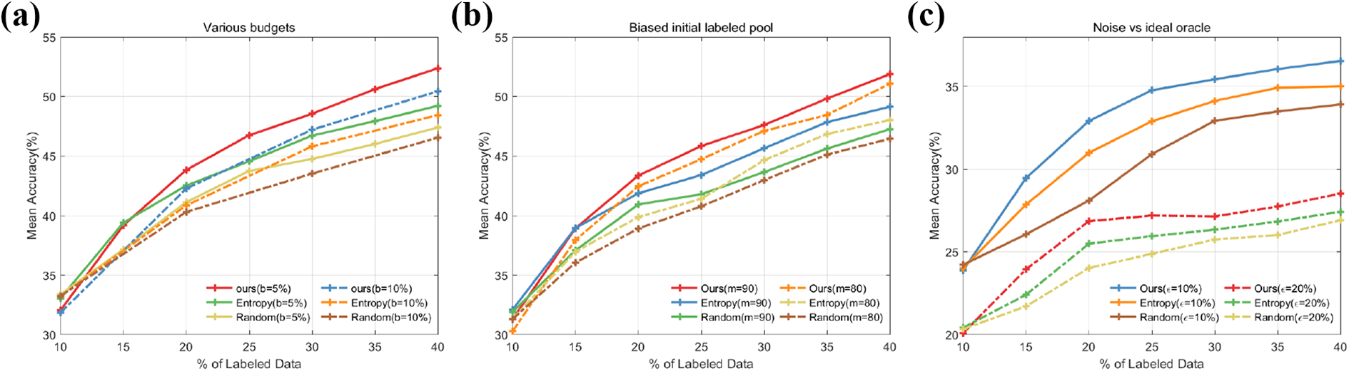
(a) to (c) Robustness of DNAL to budget size, biased initial labeled pool, and noisy labels on CIFAR-100. DNAL: double-branch deep network active learning; CIFAR: Canadian Institute for Advanced Research.

Effect of biased initial labels in DNAL

Since the bias in the initial pool might cause the inadequate representation of the data distribution, intuitively, the better the initial labeled pool we adopt, the better performance we might achieve, especially in the beginning. We define the different biases in the initial labeled pool by only providing labels from m chosen classes at random. Since there are 100 classes on the CIFAR-100 data set, we compare the performances between two different biased initial labeled pools: m = 80 and m = 90, which means we only randomly choose the initial data from 80 classes and 90 classes, respectively. Figure 8(b) shows the effect of the bias on performance based on our approach. To m = 80 and m = 90, we find that the performance of the former is always better than the latter, and in the last cycle, it is about 0.8% higher than the latter, Moreover, it can be seen that the choice of different bias does not affect the performance gap between DNAL and other baselines, indicating the robustness of our approach under different biased initial labels pool.

Noisy versus ideal oracle in DNAL

In practical AL, the labeled data might not be ideal, meaning there are some noisy data caused by an inaccurate oracle. Intuitively, the worse labeled data we adopt, the lower performance we might achieve. Since in CIFAR-100 data set, the 100 classes can be divided into 20 superclasses, meaning each image comes with a fine label and a coarse label. We define different noise in the labeled pool by changing $ε %$ data of the training set from the ground truth labels to an incorrect label but within the same superclass. Figure 8(c) shows the effect of noise on performance based on our approach by changing 10% and 20% of the training set. To $ε = 10$ and $ε = 20$ , we find that the performance of the former is always better than the latter, and in the last cycle, it is about a large margin 5.42% higher than the latter, Moreover, it can also be seen that the different noisy does not affect the performance gap between DNAL and other baselines, indicating the robustness of our approach. Intuitively, as the percentage of noisy labels increases, performances of all of the AL baselines will decrease and might converge to the same level.

Operation time analysis

In this subsection, we will take the training time and sampling time as an example to reflect the performance of time consumption over different approaches, and we use the same method to load data based on PyTorch for a fair comparison. Note that the training time gradually increases because the number of the labeled pool increases at each stage; in contrast, the sampling time gradually decreases because the number of the unlabeled pool decreases at each stage. We just list the first sampling time and training time, which means select 2500 data points from 45,000 training data set and training the total 5000 data points.

Table 1 presents our comparison for DNAL and other baselines on CIFAR-100 and we can consider random sampling strategy as an effective baseline. During the training stage, the training time of random, MC-Dropout, and Entropy methods is nearly the same (around 435 s), the reason might be that the networks for training are the same. DNAL and LLAL are at the same level and DNAL is a little higher than LLAL, and it is because the loss calculation is different during training. Note that we do not show the result of the VAAL method here since the training is too long, which might cost a few hours. For the sampling stage, we find that our approach (DNAL) achieves the competitive result, which is only 6.32 s. Moreover, MC-Dropout costs about 80 s in sample selection, because it repeats the forward network to measure the uncertainty from 10 dropout masks, and the Core-set needs about 74 s to solve an optimization problem for sample selection. Therefore, the above results indicate the complexity of our approach is competitive and demonstrate the efficient learning performance of our approach.

Table 1.

Time consumption for training stage from the labeled set and sampling stage from the unlabeled pool data set on CIFAR-100.

Method	Training time (s)	Sampling time (s)
Random	434.90	0.40
MC-Dropout	435.21	80.02
Entropy	434.85	7.85
Core-set	562.77	74.13
LLAL	724.57	6.38
DNAL (Ours)	732.21	6.32

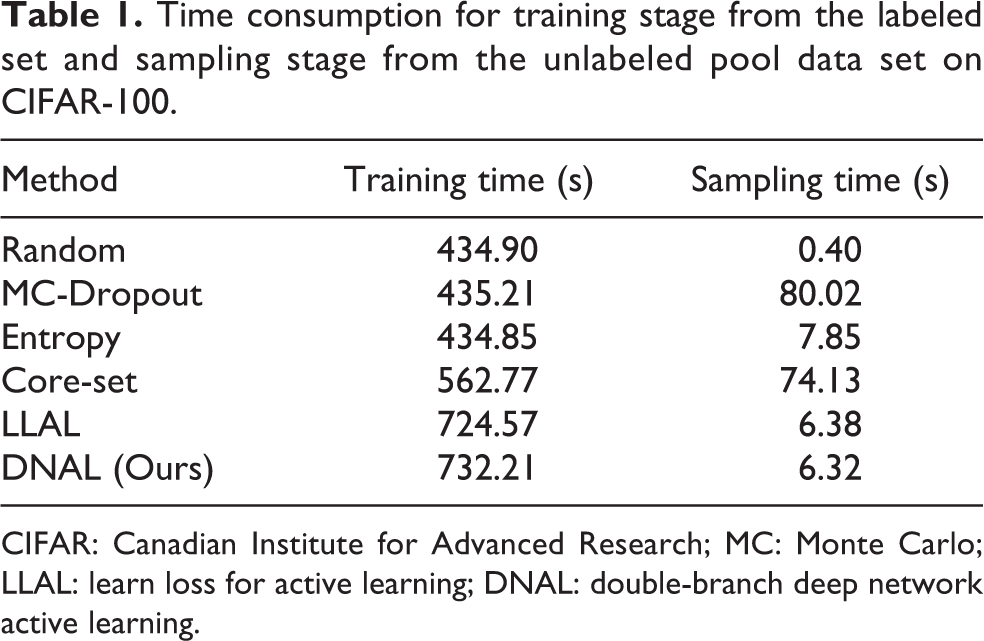
CIFAR: Canadian Institute for Advanced Research; MC: Monte Carlo; LLAL: learn loss for active learning; DNAL: double-branch deep network active learning.

Conclusions and future work

In this article, we have proposed a novel model to learn the loss for AL using a double-branch deep network. The proposed system could improve the performance for AL. Experimental results in many tasks demonstrate that the proposed approach is efficient compared with previous AL methods. Our future work includes considering the diversity or density of data to design a better architecture or extending the approach to the stream-based AL.

Supplemental material

Supplemental Material, sj-pdf-1-arx-10.1177_17298814211044930 - Loss-based active learning via double-branch deep network

Supplemental Material, sj-pdf-1-arx-10.1177_17298814211044930 for Loss-based active learning via double-branch deep network by Qiang Fang, Xin Xu and Dengqing Tang in International Journal of Advanced Robotic Systems

Footnotes

Declaration of conflicting interests

The author(s) declared no potential conflicts of interest with respect to the research, authorship, and/or publication of this article.

Funding

The author(s) disclosed receipt of the following financial support for the research, authorship, and/or publication of this article: This work was supported by the National Natural Science Foundation of China (Grant Nos. 61703418 and 61825305).

ORCID iD

Qiang Fang

Supplemental material

Supplemental material for this article is available online.

References

Liu

, et al. Semi-supervised deep coupled ensemble learning with classification landmark exploration. IEEE Trans Image Process 2020; 29: 538–550.

Wang

Zhang

, et al. Cost-effective active learning for deep image classification. IEEE Trans Circuits Syst Video Technol 2017; 27(12): 2591–2600.

Liu

Ouyang

Wang

, et al. Deep learning for generic object detection: a survey. Int J Comput Vis 2020; 128: 261–318.

Wang

Lin

Yan

, et al. Cost-effective object detection: active sample mining with switchable selection criteria. IEEE Trans Neural Netw 2019; 30(3): 834–850.

Liu

Luo

, et al. Deep learning markov random field for semantic segmentation. IEEE Trans Pattern Anal Mach Intell 2017; 40(8): 1814–1828.

Zhou

. A brief introduction to weakly supervised learning. Natl Sci Rev 2018; 5(1): 44–53.

Sundin

Schulam

Siivola

Active learning for decision-making from imbalanced observational data. In: International conference on machine learning, Long Beach, California, USA, 9–15 June 2019, pp. 6046–6055.

Wang

Dong

, et al. Joint active learning with feature selection via cur matrix decomposition. IEEE Trans Pattern Anal Mach Intell 2019; 41(6): 1382–1396.

. Pool-based sequential active learning for regression. IEEE Trans Neural Netw 2019; 30(5): 1348–1359.

10.

Lin

Huang

. Active learning for regression using greedy sampling. Inform Sci 2019; 474: 90–105.

11.

Coletta

LFS

Ponti

Hruschka

, et al. Combining clustering and active learning for the detection and learning of new image classes. Neurocomputing 2019; 358: 150–165.

12.

Wang

Hwang

Rose

, et al. Uncertainty-based active learning via sparse modeling for image classification. IEEE Trans Image Process 2019; 28(1): 316–329.

13.

Gilad-Bachrach

Navot

Tishby

. Query by committee made real. In: Proceedings of the 18th International Conference on Neural Information Processing Systems, December 2005, pp. 443–450.

14.

Settles

. Active learning. Synth Lect Artif Intell Mach Learn 2012; 6(1): 1–11.

15.

Gal

RI Y

Ghahramani

. Dropout as a bayesian approximation: representing model uncertainty in deep learning. In: International conference on machine learning, New York City, NY, USA, 19–24 June 2016, pp. 1050–1059.

16.

Gal

Islam

Ghahramani

. Deep bayesian active learning with image data. International Conference on Machine Learning, 2017, pp. 1183–1192.

17.

Walmsley

Smith

Lintott

. Galaxy zoo: probabilistic morphology through bayesian cnns and active learning. Mon Notices Royal Astron Soc 2020; 491(2): 1554–1574.

18.

Sener

Savarese

. Active learning for convolutional neural networks: a core-set approach. In: Conference: 6th International Conference on Learning Representations , ICLR 2018, April 30, 2018 - May 3, 2018, pp. 142–150.

19.

Sinha

Ebrahimi

Darrell

Variational adversarial active learning. In: International conference on computer vision, Seoul, Korea (South), 27 October–2 November 2019, pp. 5971–5980.

20.

Yoo

Kweon

IS.

Learning loss for active learning. In: The IEEE conference on computer vision and pattern recognition (CVPR), Long Beach, CA, USA, 15–20 June 2019, pp. 93–102.

21.

Joshi

Porikli

Papanikolopoulos

. Multi-class active learning for image classification. In: 2009 IEEE Computer Society Conference on Computer Vision and Pattern Recognition Workshops, CVPR Workshops 2009, pp. 2372–2379.

22.

Mnih

Kavukcuoglu

Silver

. Human-level control through deep reinforcement learning. Nature 2015; 518(7540): 529–533.

23.

Miyato

ichi Maeda

Koyama

, et al. Virtual adversarial training: a regularization method for supervised and semi-supervised learning. IEEE Trans Pattern Anal Mach Intell 2019; 41(8): 1979–1993.

24.

Krizhevsky

. Learning multiple layers of features from tiny images. MSc thesis, 2009.

25.

Griffin

Holub

Perona

. Caltech-256 object category dataset. California institute of technology, 2007.

26.

Deng

Dong

Socher

, et al. A large-scale hierarchical image database. In: Computer vision and pattern recognition, Miami, FL, USA, 20–25 June 2009, pp. 248–255.

27.

Simonyan

Zisserman

. Very deep convolutional networks for large-scale image recognition. 2014.

28.

Everingham

Gool

Winn

, et al. The pascal visual object classes (voc) challenge. Int J Comput Vis 2010; 4(7): 303–338.

29.

Liu

Anguelov

Erhan

, et al. SSD: single shot multibox detector. In: European conference on computer vision, Amsterdam, The Netherlands, 11–14 October 2016, pp. 21–37.

Supplementary Material

Please find the following supplemental material available below.

For Open Access articles published under a Creative Commons License, all supplemental material carries the same license as the article it is associated with.

For non-Open Access articles published, all supplemental material carries a non-exclusive license, and permission requests for re-use of supplemental material or any part of supplemental material shall be sent directly to the copyright owner as specified in the copyright notice associated with the article.

0.00 MB

0.07 MB