Sage Journals: Discover world-class research

Abstract

Generating a collision-free and dynamically feasible trajectory with a better clearance in a cluttered environment is still a challenge. We propose two dynamically feasible B-spline based rapidly exploring random tree (RRT) approaches, which are named DB-RRT and FMDB-RRT, to achieve path planning and trajectory planning simultaneously for omnidirectional mobile robots. DB-RRT combines the convex hull property of the B-spline and RRT’s rapid expansion capability to generate a safe and dynamically feasible trajectory. Firstly, we analyze the tree’s sustainable growth ability and put forward the dynamically feasible region. A geometric method is proposed to judge whether finding a dynamically feasible trajectory quickly. Secondly, we design two steer functions to guide the tree’s growth, improve efficiency, and decrease the number of iterations. To further increase the clearance and reduce the randomness of the trajectory, we propose FMDB-RRT, which uses the path of fast marching to guide the rapid growth of DB-RRT. Then, assuming that the number of sampled points is sufficient to represent the dynamically feasible region, the DB-RRT is proved to be probabilistically complete. Finally, by conducting experimental comparisons with other algorithms in different environments and deploying the proposed algorithm to an omnidirectional mobile robot, the effectiveness and good performance of the algorithm have been verified.

Keywords

Path planning trajectory planning rapidly exploring random tree omnidirectional mobile robots uniform B-spline fast marching method

Introduction

The modern manufacturing industry often changes products and production lines to react faster to market changes. Compared with the traditional automated guided vehicle, the autonomous omnidirectional mobile robot is more flexible and can better adapt to the production process of modern manufacturing.^1,2 Motion planning, as a bridge connecting perception and control, is the cornerstone for robots to realize autonomous navigation.^3,4

Many motion planning algorithms have been proposed. The search-based planning algorithms, such as Dijkstra⁵ and A*,⁶ can find the optimal trajectory with respect to discretization. Some variants^7
–9 have been put forward to solve kinodynamic planning. However, computation time and memory usage of search-based planning approaches will rise exponentially with the increase of the state-space dimensionality. Nonlinear optimization-based methods^10
–12 use nonlinear optimization to handle the trajectory optimization problem using the gradient information of the environment. However, there is no theoretical guarantee that the obtained trajectory must not collide with obstacles. These methods also have local minimum problems. Sampling-based exploring algorithms, such as rapidly exploring random tree (RRT)¹³ with its variants¹⁴ and probabilistic roadmap,¹⁵ are capable of solving the motion planning problem with complex constraints and can save computation, attracting more and more researchers’ attention.¹⁶ However, generating a safe and dynamically feasible trajectory with a better clearance in a cluttered environment is still a challenge.

To solve the above problems, we propose DB-RRT and FMDB-RRT to achieve path planning and trajectory planning simultaneously for omnidirectional mobile robots. The contributions of this work are as follows:

DB-RRT combines the convex hull property of the B-spline and RRT’s rapid expansion capability to generate a safe and dynamically feasible trajectory. With a mild assumption, the DB-RRT is proved to be probabilistically complete.

In the case where the velocity and acceleration control points of the initial state meet the dynamical limits, we analyze the DB-RRT’s sustainable growth ability. A geometric method is proposed to determine whether a dynamically feasible trajectory is found quickly.

To reduce the number of iterations, two steer functions are designed to guide the tree growth. To further increase the clearance and reduce the randomness of the trajectory, we propose FMDB-RRT, which uses the path of fast marching (FM) to guide the rapid growth of DB-RRT.

The remainder of this article is organized as follows. The related works are introduced in the second section. In the third section, we introduce the velocity and acceleration space of the omnidirectional mobile robot and the basic uniform B-spline concept firstly. Secondly, we explain the essential functions of DB-RRT in detail. Then, we explain the strategy of using the path of FM to guide the growth DB-RRT. At the end of this section, we analyze the probability completeness of DB-RRT. In the fourth section, we conduct experimental comparisons and apply the algorithm to an omnidirectional mobile robot. We give the conclusion and future work in the fifth section.

Related works

Although RRT,¹³ as the successful single-query method, has a tortuous and nonoptimal path. Some optimization or pruning methods are proposed to get a shorter or optimal path. RRT*¹⁷ uses branch trimming and rewiring mechanisms to ensure asymptotic optimality. RRT*-Smart¹⁸ employs intelligent sampling and path trimming to obtain optimal or near-optimal path. P-RRT*¹⁹ introduces artificial potential field (APF) to providing a direction for exploration, obtaining a quicker convergence. RRT*-SV²⁰ uses the Sukharev grids and convex vertices to enhance the sampling process, reducing planning time. The asymptotical optimality of Kinodynamic RRT*²¹ has been proved, but complicated calculations cause it to not run in real time. In the literature,²² a method was proposed for the RoboCup robot by adding gravitational components and path smoothing strategies to Bi-RRT, reducing the randomness and the length of the path. The path obtained by the above algorithms is often short. However, ignoring distance to the obstacle, the obtained path is often unsafe for the robot. When the robot executes this kind of path, it is easy to scratch with the obstacle due to the uncertainty of positioning and execution.^23,24

Some path-biasing approaches have been presented to decrease planning time and enhance path quality. In the literature,²⁵ a hierarchical planning algorithm was proposed by focusing the RRT* growing in the high-dimensional state space along an initial path. Theta*-RRT²⁶ combines any-angle search with RRT for nonholonomic wheeled robots. However, those methods’ initial path does not consider the clearance with obstacles so that they may generate a path close to the obstacle. The Skilled-RRT²⁷ method was proposed to solve the problem, which can be used for path planning of nonholonomic and holonomic robots in the building environment. This method first extracts the shortest path in the skeleton of the environment and grows the RRT along this path quickly. As the Skilled-RRT extracts the shortest path on the environment skeleton, the obtained path does not always have a better clearance. Moreover, Skilled-RRT only considers the velocity constraint, and velocity is not continuous, which makes Skilled-RRT not suitable for massive robots or vehicles. Our method can get a trajectory with better clearance, which is also a safer trajectory. Moreover, our method can generate a dynamically feasible trajectory with continuous acceleration.

There are some works combining RRT and spline. In the literature,²⁸ a method was proposed using a spline to smooth the path obtained by RRT, and the path can be better tracked by the vehicle. However, the path after smooth deviating from the RRT path may collide with obstacles. Some works^29
–31 aim to plan a path for mobile robots or vehicles with differential constrain. In the literature,³¹ a motion planning algorithm for autonomous vehicles was presented, which employs two B-spline search trees to generate a continuous and feasible path. SRRT³⁰ uses spline curve parameterization to generate continuous curvature path satisfying curvature constraints. Unlike the above works, we solve the problem of path planning and trajectory planning simultaneously of holonomic robots and directly obtain the time-parameterized dynamically feasible trajectory.

Unlike the above method, we propose two novel methods combining B-spline and RRT, which can simultaneously achieve path planning and trajectory planning for omnidirectional mobile robots within a reasonable time. The generated trajectory satisfies the dynamic constraints so that the omnidirectional robot can execute it without further velocity planning. Besides, different from the path-guided method mentioned earlier, the proposed FMDB-RRT method can obtain better clearance in a cluttered environment.

Dynamically feasible B-spline based rapidly random tree

Omnidirectional mobile robot and uniform B-spline

The omnidirectional mobile robot can be independently planned in three directions.³² Due to the unique structure, a velocity range that satisfies $v_{i} \in [- v_{max}, v_{max}]$ and angular velocity range that satisfies $ω \in [- ω_{max}, ω_{max}], i \in {x, y}$ can be found in its velocity space. Acceleration $a_{i},$ and angular acceleration $α, i \in {x, y}$ have similar restrictions^33,34 as velocity. When the orientation is unchanged during the movement, the ranges of velocity and acceleration in the x-y direction can become larger, making the robot moving faster. In some practical applications, when the robot arrives at the location, it adjusts its direction according to handling requirements. Based on the above considerations, during the robot’s movement, we keep the robot’s rotation unchanged. In this way, the constraints of velocity and acceleration can be regarded as two independent rectangles $v_{i} \in [- v_{max}, v_{max}]$ and $a_{i} \in [- a_{max}, a_{max}], i \in {x, y}$ .

A p’th B-spline is defined by N+1 control points {P₀, P₁,…P_N}, $P_{i} \in R^{2}$ , and knot vector [t₀, t₁,…t_M] $t_{m} \in R$ , where M = N + p + 1. A uniform B-spline, as a kind of B-spline, is parameterized by time t, and $t \in [t_{p}, t_{M - p}]$ with each knot span has identical value Δt. To get the position at the corresponding time, t is normalized as $α (t) = (t - t_{m}) / Δ t$ , where $t \in [t_{m}, t_{m + 1}] \subset [t_{p}, t_{M - p}]$ . Then, the position can be evaluated using the matrix representation³⁵

\begin{array}{l} p (α (t) = α {(t)}^{T} M_{p + 1} P \\ α (t) = {[α^{p} (t), α^{p - 1} (t), \dots α (t), 1]}^{T} \\ P = {[P_{i - p}, P_{i - p + 1}, P_{i - p + 2}, \dots, P_{i}]}^{T} \end{array}

where $M_{p + 1}$ is constant matrix determined by p. We choose the cubic uniform B-spline in this work as it can guarantee the continuity of velocity and acceleration. B-spline has a convex hull property, which means that all control points are restricted to a convex hull, and the derivative of B-spline is still B-spline. $V_{i}, i \in [0, N - 1]$ and $A_{i}, i \in [0, N - 2]$ represent the velocity control points and acceleration control points, respectively

V_{i} = (P_{i + 1} - P_{i}) / Δ t, A_{i} = (V_{i + 1} - V_{i}) / Δ t

If the control points are known, we can get velocity control points, acceleration control points using equation (2), where $Δ t$ is the knot span. As shown in Figure 1, as long as we constrain all velocity control points within $v_{i} \in [- v_{max}, v_{max}], i \in {x, y}$ and acceleration control points within $a_{i} \in [- a_{max}, a_{max}], i \in {x, y}$ , then the generated trajectory must meet the dynamical limits.

Figure 1.

(a–c) Due to the convex hull characteristic of cubic uniform B-spline, the velocity and acceleration can be limited to a certain range.

Overview of DB-RRT

In Figure 2, the left part shows the process of DB-RRT growth. The right part of Figure 2 shows the selection process of $x_{new}$ , which will be introduced in “Different steer function” section. The pseudocode of DB-RRT is shown in Algorithm 1. We utilize the control points P of B-spline as the RRT node and the connection between the control points as the edge. M represents the environment, and Δt is the knot of uniform B-spline. ${State}_{init}$ and ${State}_{goal}$ refer to initial state and goal state, respectively. $k, d_{min}$ and SampleNum will introduce in “Different steer function” section. Dynlimits refers to the maximum acceleration and velocity restraints in the x-y directions. Using the ComputeControlPoints function, which calculates control points, the initial and goal state control points can be calculated (lines1,2). DynamicallyFeasibleCheck is used to judge whether the velocity control points and acceleration control points derived from the calculated control points meet dynamical limits. If these control points do not meet dynamical limits, a reasonable initial state and goal state need to be provided (lines 3,4). When the tree grows, unlike the normal RRT algorithm, we also store the control points related to initial state and goal state.

Figure 2.

The left part shows the process of DB-RRT growth. The blue line is the edge of the DB-RRT, and the green line is the B-spline curve. At this time, the iteration number is 63, and there are 38 nodes in the tree. The right side is an enlarged view of part of the left part showing the selection process of $x_{new}$ .

Algorithm 1

DB-RRT algorithm.

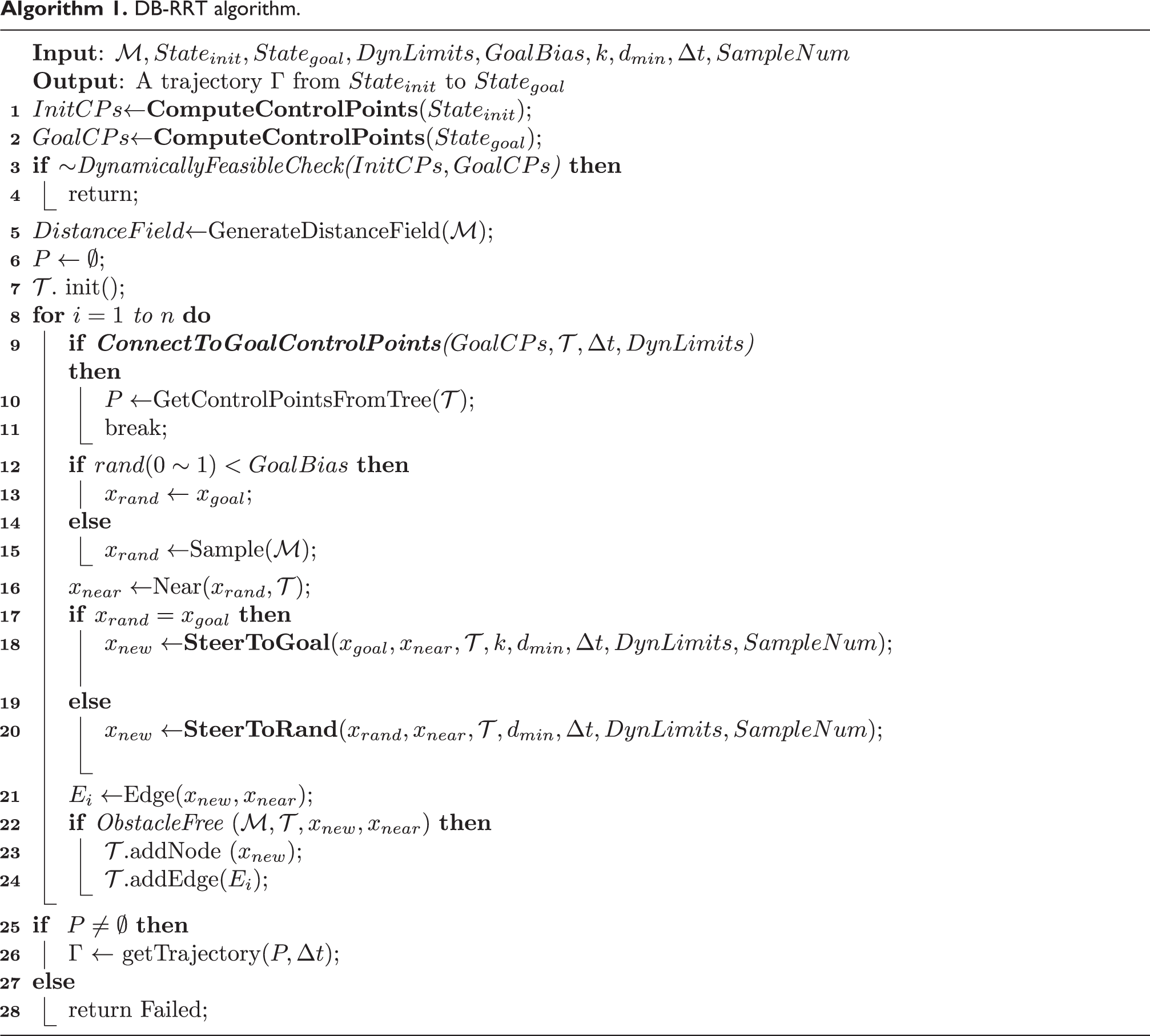
The ConnectToGoalControlPoints function is designed to determine whether the newly added node can connect to the control points of the goal state (lines 9–11). If successful, the dynamically feasible trajectory is obtained, the algorithm ends (lines 25,26). If not, the tree continues to grow until the dynamically feasible trajectory is successfully found or the number of nodes that reach the maximum expansion limit returns planning failure (lines 27,28). The ConnectToGoalControlPoints function will be described in detail in “Quickly determine whether finding a trajectory” section. The sampling process and finding the nearest node are the same as the RRT algorithm (lines 12–16).

We designed different steer functions for biasing to goal state or $x_{rand}$ (lines 17–20). These two functions use the distance field (line 5) to select the collision-free $x_{new}$ . We will introduce these two functions in detail in “Different steer function” section. The ObstacleFree function detects whether the edges of the $x_{new}$ node and the $x_{near}$ node collide with obstacles. It also detects whether the newly generated piecewise B-spline collides with obstacles (line 22). The process of adding nodes and edges is the same as the RRT algorithm (lines 23,24).

Analysis of the sustainable growth of DB-RRT

In this part, we give an analysis that the tree can grow continuously. It is assumed that the velocity control points and acceleration control points derived from the current control points satisfy dynamic constraints. Then, a new control point must be added to get a new piecewise B-spline, and the velocity control points and acceleration control points derived from this new added control point still meet the dynamical limits.

As shown in Figure 3, it is assumed that the velocity and acceleration control points derived from P_i, $P_{i + 1}$ , and $P_{i + 2}$ satisfy dynamic constraints. $P_{i + 3}$ is the newly added control point. According to equation (2), the above control points can get the following velocity and acceleration control points

\begin{array}{l} V_{i} = (P_{i + 1} - P_{i}) / Δ t, V_{i + 1} = (P_{i + 2} - P_{i + 1}) / Δ t, V_{i + 2} = (P_{i + 3} - P_{i + 2}) / Δ t \\ A_{i} = (P_{i + 2} - 2 P_{i + 1} + P_{i}) / Δ t^{2}, A_{i + 1} = (P_{i + 3} - 2 P_{i + 2} + P_{i + 1}) / Δ t^{2} \end{array}

where $V_{i + 2}$ and $A_{i + 1}$ are derived from the new control point $P_{i + 3}$ , which need to meet the following dynamical limits

\{\begin{cases} - v_{max} \leq V_{i + 2} = (P_{i + 3} - P_{i + 2}) / Δ t \leq v_{max} \\ - a_{max} \leq A_{i + 1} = (P_{i + 3} - P_{i + 2} + P_{i + 1}) / Δ t^{2} \leq a_{max} \end{cases}

Figure 3.

The newly added control point and its value range.

From equation (4), the value range of P_i+3 can be obtained

P_{i + 2} - v_{max} Δ t \leq P_{i + 3} \leq P_{i + 2} + v_{max} Δ t

2 P_{i + 2} - P_{i + 1} - a_{max} Δ t^{2} \leq P_{i + 3} \leq 2 P_{i + 2} - P_{i + 1} + a_{max} Δ t^{2}

When P_i+3 takes a value within the above range, the derived velocity and acceleration control points must satisfy the dynamic constraints. In Figure 3, the red rectangle represents the range of P_i+3 determined by equation (5). The blue rectangle represents the range of P_i+3 determined by equation (6). The shaded part represents the intersection of equations (5) and (6). The critical question is whether the shaded part, representing the value range of P_i+3, always exists.

According to the counter-proof method, we know that value range of P_i+3 does not exist when any of the following equations are satisfied

2 P_{i + 2} - P_{i + 1} - a_{max} Δ t^{2} > P_{i + 2} + v_{max} Δ t

P_{i + 2} - v_{max} Δ t > 2 P_{i + 2} - P_{i + 1} + a_{max} Δ t^{2}

For equation (7), move $P_{i + 2}$ to the left of the equation

P_{i + 2} - P_{i + 1} - v_{max} Δ t > a_{max} Δ t^{2}

As $P_{i + 2} - P_{i + 1} \leq v_{max} Δ t$ on the left side of the inequality, we can get $P_{i + 2} - P_{i + 1} - v_{max} Δ t \leq 0$ . However, on the right side of the inequality, we can get $a_{max} Δ t^{2} > 0$ . After the above analysis, we can see that this inequality is not satisfied. Similarly, equation (8) has the same conclusion.

In conclusion, if the current control point satisfies dynamic constraints, then a new control point can be added to get a new part B-spline. The velocity control points and acceleration control points derived from this new control point still meet the dynamical limits. Because the control points related to initial state satisfy the constraints, it means that the tree must continue to expand.

For the convenience of description, we will name the value range of the control point P_i+3 as the dynamically feasible region in the rest of this article. The dynamically feasible region is essential in our work. In Figure 3, the dynamically feasible region of P_i+3 is indicated by the blue shading region. In “Quickly determine whether finding a trajectory” section, we use the dynamically feasible region to determine whether the trajectory is found. In “Different steer function” section, the nodes selected in the dynamically feasible region must satisfy the dynamic constraints, and no additional calculation is required.

Quickly determine whether finding a trajectory

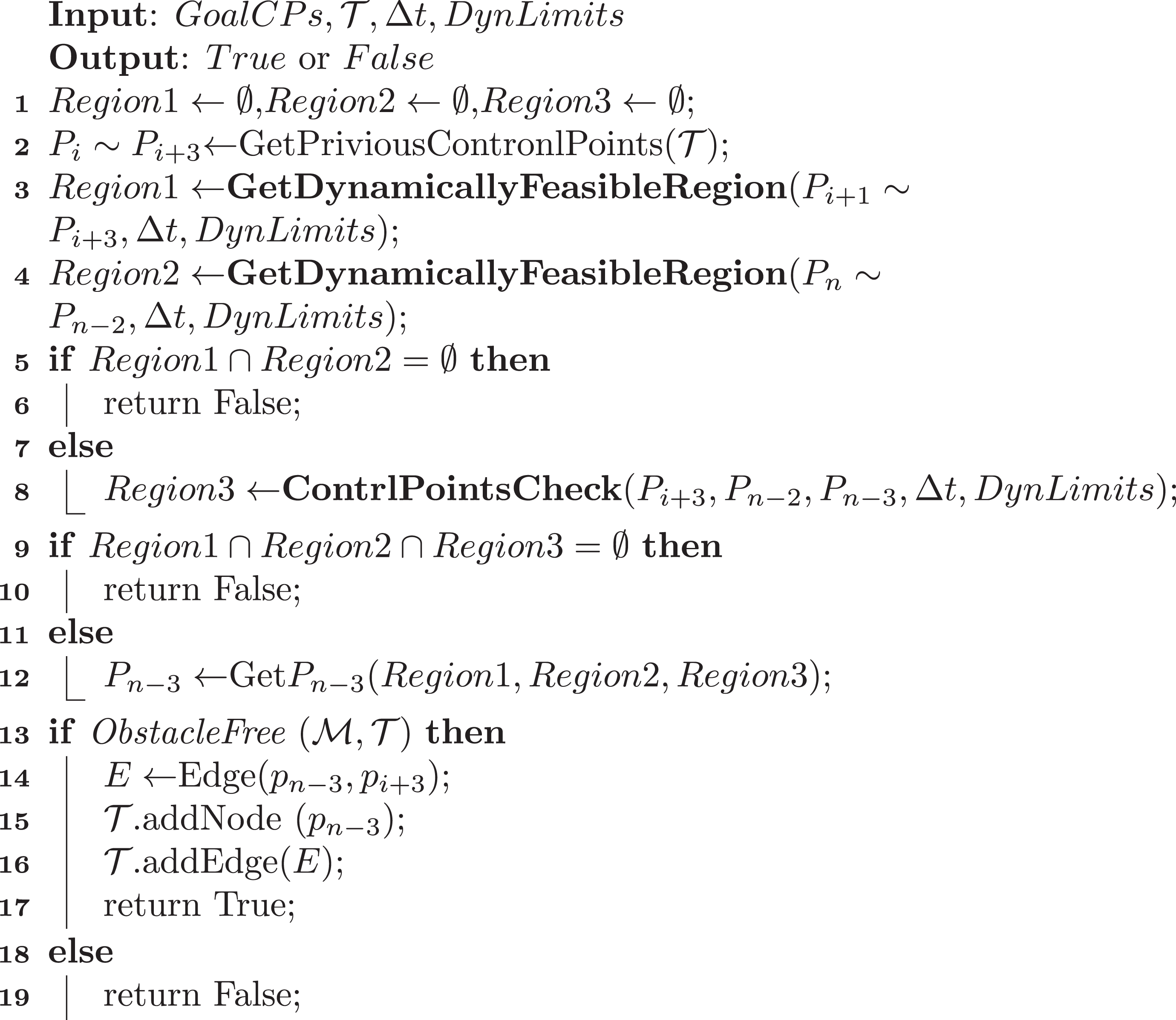
Based on the proposed dynamically feasible region, we propose a geometric method to determine whether the newly added node can quickly connect to the goal state’s control points, which is used to judge whether a dynamically feasible trajectory is found. Algorithm 2 shows the pseudocode of ConncetToGoalControlPoints function.

Algorithm 2

ConnectToGoalControlPoints.

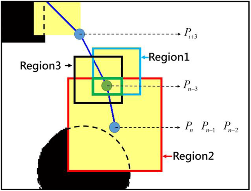
As shown in Figure 4, P_n, $P_{n - 1}$ , $P_{n - 2}$ , and $P_{n - 3}$ (n ≥ 3) are the goal state’s corresponding control points. $P_{n - 3}$ is the fourth control point from the end, indicated by a green dot in Figure 4. Because the goal state is set to static in this case, the control points P_n, P_n-1, and P_n-2 are coincident, indicated by blue dots in Figure 4. $P_{i + 3} (i > = 0)$ is the newly added node, indicated by blue dots in Figure 4. P_i, $P_{i + 1}$ , and $P_{i + 2}$ are former parent nodes of P_i+3. Due to the size limitation of the figure, only P_i+3 is shown in Figure 4.

Figure 4.

Black regions are obstacles, and yellow regions indicate dynamically feasible regions. Schematic diagram of the connection between the newly added node $P_{i + 3}$ and control points of the goal state which are P_n, $P_{n - 1}$ , $P_{n - 2}$ , and $P_{n - 3}$ . Determine whether the dynamically feasible trajectory is found by judging whether the three regions overlap.

This ConncetToGoalControlPoints function is used to determine whether the newly added node P_i+3 can connect to $P_{n - 3}$ with the derived velocity control points and acceleration control points meeting dynamical limits. Based on the previous section’s discussion, we transformed this into a problem to determine whether the dynamically feasible regions overlap.

The GetPriviousControlPoints function can get the newly added node and the previous three nodes (line 2). The GetDynamicallyFeasibleRegion function based on equation(10) can calculate the dynamically feasible region of the next control point through nodes P_i+3, $P_{i + 2}$ , and $P_{i + 1}$ , which is named region1 (line 3). In Figure 4, region1 is represented by a blue square

\{\begin{cases} P_{i + 3} - v_{max} Δ t \leq P_{n - 3} \leq P_{i + 3} + v_{max} Δ t \\ 2 P_{i + 3} - P_{i + 2} - a_{max} Δ t^{2} \leq P_{n - 3} \leq 2 P_{i + 3} - P_{i + 2} + a_{max} Δ t^{2} \end{cases}

Similarly, based on equation (11), we can calculate the dynamically feasible region of the next control point through P_n, P_n-1 , and P_n-2, which is named region2 (line 4). In Figure 4, region2 is represented by a red square

\{\begin{cases} P_{n - 2} - v_{max} Δ t \leq P_{n - 3} \leq P_{n - 2} + v_{max} Δ t \\ 2 P_{n - 2} - P_{n - 1} - a_{max} Δ t^{2} \leq P_{n - 3} \leq 2 P_{n - 2} - P_{n - 1} + a_{max} Δ t^{2} \end{cases}

If region1 and region2 overlap, further judgment is made, otherwise false is returned (lines 5,6).

The ControlPointsCheck function ensures that the derived velocity and acceleration control points related to $P_{i + 3}$ and $P_{n - 3}$ meet the dynamical limits. We get a new dynamically feasible region, which is named region3 (line 8). Region3 is represented by black squares in Figure 4. The ControlPointsCheck function is based on the following analysis.

Figure 5 shows the affected nodes, which can be divided into four groups. After the above discussion, control points in the first and fourth groups must meet the dynamical limits. It is only necessary to judge whether the velocity control points and acceleration control points derived from control points in the second and third groups meet the dynamical limits. At this time, only $P_{n - 3}$ is a variable, and we can get the inequality of P_n-3. Remove the constraint that repeats with equation (12), we get the following constraints

(P_{i + 3} + P_{n - 2} - a_{max} Δ t^{2}) / 2 \leq P_{n - 3} \leq (P_{i + 3} + P_{n - 2} + a_{max} Δ t^{2}) / 2

Figure 5.

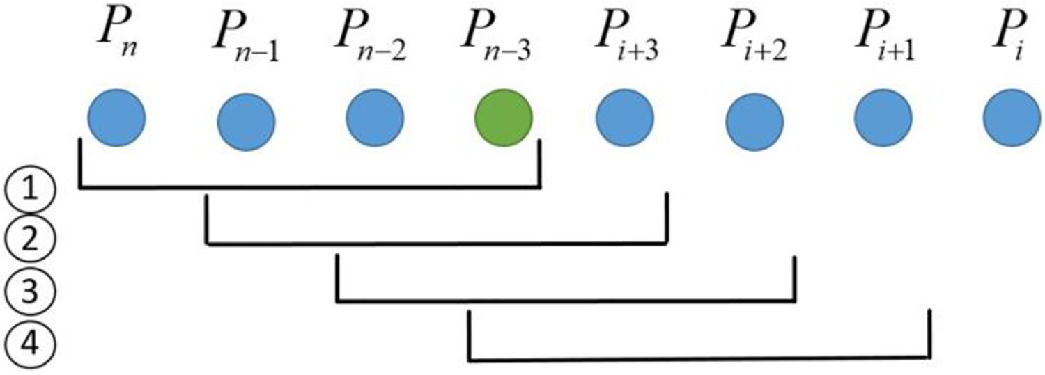
The affected nodes can be divided into four groups.

If the intersection of region1, region2, and region3 is empty, return false (lines 9,10). If the intersection of region1, region2, and region3 is not empty, select the center of the intersection of the three regions as P_n-3 (line 12). The green rectangular area in Figure 4 represents the intersection of region1, region2, and region3. If there is no collision with obstacles, then add the corresponding nodes and edges to the tree and output true. Otherwise, false is output. It should be noted that this function can also ensure the trajectory obtained by our algorithm indeed reach the goal state.

Different steer function

Considering the efficiency and effect, we have designed two different functions to find $x_{new}$ , which are used to guide the growth of tree toward $x_{rand}$ or goal state.

SteerToRand function

The SteerToRand function is used to guide the growth of tree toward $x_{rand}$ by generating $x_{new}$ in the dynamically feasible region. The GetDynamicallyFeasible function uses $x_{near}$ and its two former parent nodes to obtain the dynamically feasible region (line 3). We first take sampleNum points uniformly in this region and then add the points that are not close to obstacles to SamplesCollisionFree (lines 4–7). The $d_{min}$ is a small value to avoid the nodes and obstacles being too close. Choose a node in SamplesCollisionFree, which is closest to $x_{rand}$ as $x_{new}$ (line 8). We use Euclidean distance to measure how close the node is to $x_{rand}$ . The control points affect the shape of B-spline. Choosing the point closest to $x_{rand}$ also corresponds to the B-spline that is most inclined to grow toward $x_{rand}$ . If the found $x_{new}$ is too close to $x_{near}$ , it often causes the velocity and acceleration to change too much in a short time. To avoid the above situation, if the distance is less than minstepsize, select the point furthest away from $x_{near}$ as $x_{new}$ (lines 9,10).

Algorithm 3

SteerToRand.

SteerToGoal function

The SteerToGoal function is used to guide the growth of the tree toward goal state by generating $x_{new}$ in the dynamically feasible region. The $x_{rand}$ only has position information, while goal state includes position, velocity, and acceleration. We calculate an optimal boundary value problem between the end state of the piecewise B-spline, which is related to each node in SamplesCollisionFree and the goal state. Select the trajectory with the smallest cost, which is also most inclined to expand toward the goal state. Solve the corresponding cost for these nodes according to equation (16) and select the node with the smallest cost as $x_{new}$ . The growing process of the tree and the selection process of $x_{new}$ are shown in Figure 2.

Algorithm 4

SteerToGoal.

We consider the omnidirectional mobile robot as a second-order integrator model. We can define the state-space model as

\begin{array}{l} \dot{s} = A \cdot s + B \cdot u \\ A = [\begin{array}{l} 1 I_{2} 0 \dots 0 \\ 0 0 I_{2} \dots 0 \\ ⋮ ⋮ ⋮ ⋱ ⋮ \\ 0 \dots \dots 0 I_{2} \\ 0 \dots \dots 0 0 \end{array}] B = [\begin{array}{l} 0 \\ 0 \\ ⋮ \\ 0 \\ I_{2} \end{array}] \end{array}

We can express state equation solution as

s (t) = e^{A t} s_{0} + \int_{0}^{t} e^{A (t - σ)} B u (σ) d σ

The s₀ and $u (t)$ represent the initial state and the control input, respectively

u (t) = (\begin{array}{l} a_{x} \\ a_{y} \end{array}), s (t) = (\begin{array}{l} p_{x} \\ p_{y} \\ v_{x} \\ v_{y} \end{array})

The cost function is designed as

J = \sum_{i \in {x,y}} J_{i}, J_{i} = \int_{0}^{T} u_{i} {(t)}^{2} d t + k T

A closed-form trajectory is computed that minimizes J from the end state of the piecewise b-spline corresponding, which is related to each node in SamplesCollisionFree to goal state using Pontryagin’s minimum principle^36,37

\begin{array}{l} J = k \cdot T + α T^{- 1} + β T^{- 2} + γ T^{- 3} \\ α = 4 ({v_{x 0}}^{2} + v_{x 0} \cdot v_{x f} + {v_{x f}}^{2} + {v_{y 0}}^{2} + v_{y 0} \cdot v_{y f} + {v_{y f}}^{2}) \\ β = 12 ((p_{x 0} - p_{x f}) \cdot (v_{x 0} + {v_{x}}_{f}) + (p_{y 0} - p_{y f}) \cdot (v_{y 0} + v_{y f})) \\ γ = 12 ({(p_{x 0} - p_{x f})}^{2} + {(p_{y 0} - p_{y f})}^{2}) \end{array}

where $p_{i 0}, p_{i f}, v_{i 0}, v_{i f}, i \in {x, y}$ denote the position and velocity of the robot’s initial state and goal state. k is the coefficient of balance trajectory time and control cost. It can be seen that J is only related to T, and the optimal trajectory can be obtained by minimizing J. The control point with the smallest J will be selected as $x_{new}$ .

Guiding the growth of DB-RRT using fast marching

The FM³⁸ is proposed by Sethian to solve wave propagation problems for image processing. As the FM method is local minimum free, it has also been used for path planning in recent years.³⁹ Figure 6 shows the steps of guiding the growth of DB-RRT using FM.

Figure 6.

The steps of guiding the growth of DB-RRT using fast marching.

To reduce the search time, we use bilinear interpolation to shrink the map and use it to generate the distance field. The centers of the dynamically feasible regions derived from the control points of initial and goal states are used as the start point and the endpoint. Using the generated distance field, FM generates a path. The forward propagation velocity of each grid point is related to its distance to the nearest obstacle. A path away from obstacles is generated to guide the expansion of DB-RRT.

We reduce the number of obtained waypoints by the following method. First, we calculate the length L of the path, and then, uniformly sample ns, $n s = L / min (v_{max} \cdot Δ T, a_{max} \cdot Δ T^{2})$ , points on the path. The angle is calculated for every three points of the above path, which represents the changes of curvature. If the angle corresponding to the path point is less than 175°, the path point is selected as the guide path. Select the points of the guide path as $x_{rand}$ to guide the tree’s growth. The newly added node is selected as $x_{near}$ . When the distance between $x_{new}$ and the guidance point is less than $1.2 min (v_{max} \cdot Δ T, a_{max} \cdot Δ T^{2})$ , then, in the next iteration, the next point of the guidance path is selected as the $x_{rand}$ . Following the above steps, the tree continues to grow toward the goal along the guide path. When the tree’s growth is blocked, clear the last generated nodes and use the DB-RRT algorithm for planning. For convenience, we name the DB-RRT guided by the path of FM as FMDB-RRT.

Probabilistic completeness analysis

Based on the discussion of “Quickly determine whether finding a trajectory” section, let q be the fourth control point from the end of any dynamically feasible collision-free goal state and $q \in C_{free}$ . The distance between q and the closest vertex in DB-RRT is presented as $D_{k} (q)$ . Let d_k indicate the value of D_k and k is the number of vertices in tree.

Lemma 1

Suppose $C_{free}$ is n-dimensional subset of an n-dimensional configuration space, in this work, n is 2. For any $q \in C_{free}$ , the dynamically feasible region of q is N and $N \cap C_{free} \neq \emptyset$ . There must be a node v_k, which derives dynamically feasible region M, $Ω \in M \cap N$ meet $lim_{k \to \infty} P (Ω \notin \emptyset) = 1$ and equation (12).

Proof

Let q be any point in $C_{free}$ , the dynamically feasible region of q is N. Let q₀denote any initial DB-RRT vertex, which derives dynamically feasible region M. With the number of samples rises, the value of k increases, d_k is getting smaller, which means more nodes close to q. Simultaneously, the probability of overlapping between the M and N approaches 1, and the probability of satisfying equation (12) approaches 1. In conclusion, as the number of k increases, there must be a node v_k, which derives dynamically feasible region M, $Ω \in M \cap N$ meet $lim_{k \to \infty} P (Ω \notin \emptyset) = 1$ and equation (12).

Theorem 1

Assume that the number of sampled points is sufficient to represent the dynamically feasible region and the DB-RRT algorithm is probabilistically complete.

Proof

Let X indicates a random variable that represents the sampling process a random variable X_k represents the DB-RRT vertices’ distribution. It is assumed that the number of sampled points is sufficient to represent the dynamically feasible region. Similar to the RRT algorithm, the growth of DB-RRT’s new node X_k is extended toward X, which does not change the randomness of the sampling. As the amount of samples increases, k approaches infinity and X_k converges to X in probability. Combined with Lemma 1, the DB-RRT satisfies uniform sampling, and as the number of samples increases, the existing trajectories satisfying the dynamic constraints can be found. In summary, DB-RRT is probabilistically complete.

When using the guided path to guide the growth of DB-RRT, no trajectory was found. The last generated nodes and edges will be cleared, and then, the DB-RRT algorithm is used for planning. This will not have any effect on the growth of DB-RRT and do not adversely affect the convergence results.

Experimental tests

The proposed algorithm is compared with RRT, RRT*,¹⁷ RRT-connect,¹⁴ and the improved RRT methods,^22,27 which are suitable for omnidirectional mobile robots. To ensure the correctness of the results, we use different types of environments for testing. In the next part, we deploy the proposed algorithm to an omnidirectional mobile robot to verify the algorithm’s effectiveness.

Comparisons and analysis

Introduction to environments and parameters

As shown in Figure 7, the first line shows randomly generating maps with obstacles of different sizes, numbers, and shapes. It should be noted that there are overlapping obstacles. The second line shows three maps representing different building environments with randomly generated obstacles. All maps have a resolution of 2 cm. We focus on seven factors: planning time, iteration number, clearance, path length, dynamic limits, execution time, and success rate. Each algorithm runs 100 times in each environment, and the results were averaged.

Figure 7.

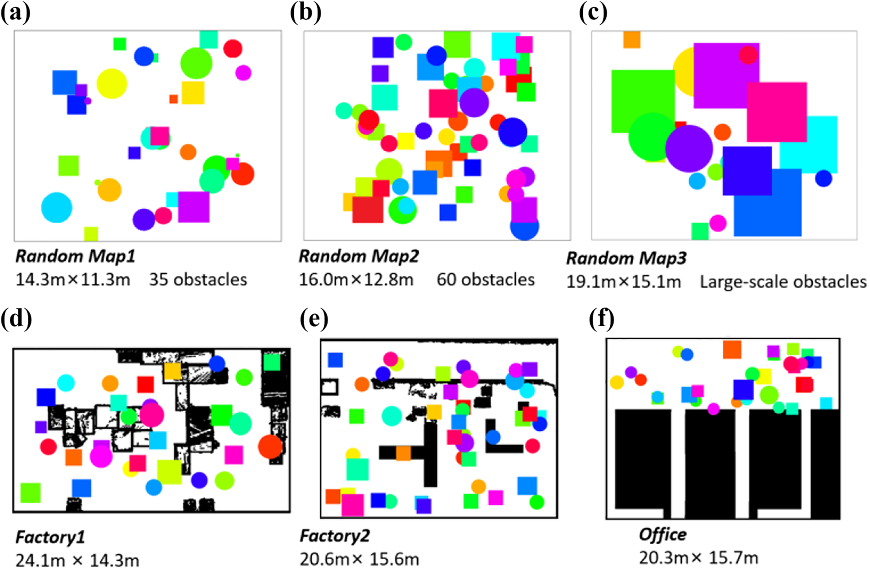
Randomly generated maps and three maps represent different building environments. (a) Random map1, (b) Random map2, (c) Random map3, (d) Factory1, (e) Factory2, and (f) office.

The parameter selection of each algorithm is introduced as follows. For RRT, RRT*, RRT-connect, and the method in the literature,²² the step size and threshold to the goal or to the other tree are set to 0.5 m. In the cluttered environment, to improve the success rate of the method in the literature,²² we set kp to 0.1. The goal bias for RRT, RRT*, the method in the literature,²² and DB-RRT is set to 10%. For DB-RRT and FMDB-RRT, the maximum acceleration and velocity in the x and y directions are set to 0.4 m/s² and 0.5 m/s. The minstepsize is set to $υ_{max} Δ t / 5$ . The dmin is set to 0.2 m in our implementation. The sampleNum is set to 25. The k is set to 1. The Δt is set to 1 s. The map used to run FM is set to one-fifth of the original size. For Skilled-RRT, we consider the environmental size and calculate the parameters according to the method proposed in the literature.²⁷ We use an omnidirectional car for calculation, where the vehicle velocity v_c is set to 0.4 m/s and delta q is set to 0.5.

Random maps are used to test RRT, RRT*, RRT-connect, the method in the literature,²² DB-RRT, and FMDB-RRT. Skilled-RRT is limited to a building environment, so we use the two environments in the factory and an office environment to compare this algorithm with other algorithms in “Experiments in building environments” section. It should be noted that the RRT-connect algorithm grows branch multiple times each cycle, which is different from the other methods. To be fair, the number of iterations in this article refers to the number of growth of RRT branches. Each algorithm sets the same maximum time limit 10 s in each environment.

All experiments are carried out on a laptop, which equipped with Intel i5-8250U CPU, 8G RAM, and 240G ROM. All codes are implemented in Matlab 2018b on Windows 10. All algorithms use the same functions that can be shared. Note that, since the above algorithms are implemented by ourselves, the comparisons may not be completely fair.

Experiments in random environments

Table 1 presents the experimental data and Figure 8 shows the performance of different algorithms in three random environments. The best value in each item is shown in bold.

Table 1.

Experimental data of different algorithms in random environments.

	Planning time (s)	Iteration number	Length (m)	Average clearance (m)	Success rate	Execution time (s)	Dynamic limits
Random map1
RRT	0.13	438	21.17	0.62	100%	—	N
Method in the literature²²	0.15	381	17.42	0.52	100%	—	N
RRT-connect	0.10	386	20.53	0.59	100%	—	N
RRT*	0.41	422	17.40	0.62	100%	—	N
DB-RRT	0.27	253	19.63	0.58	100%	41	Y
FMDB-RRT	0.24	37	21.06	1.04	100%	40	Y
Random map2
RRT	0.41	1533	33.07	0.62	100%	—	N
Method in the literature²²	0.41	1385	26.70	0.38	100%	—	N
RRT-connect	0.29	1569	31.09	0.52	100%	—	N
RRT*	1.47	1496	25.95	0.53	100%	—	N
DB-RRT	1.07	1281	33.37	0.59	100%	68	Y
FMDB-RRT	0.26	57	30.23	0.87	100%	60	Y
Random map3
RRT	0.43	1583	31.60	0.56	100%	—	N
Method in the literature²²	0.55	2021	27.01	0.56	100%	—	N
RRT-connect	0.35	1916	31.80	0.51	100%	—	N
RRT*	1.70	1709	26.46	0.59	100%	—	N
DB-RRT	0.56	621	29.48	0.52	100%	57	Y
FMDB-RRT	0.26	53	28.31	0.94	100%	56	Y

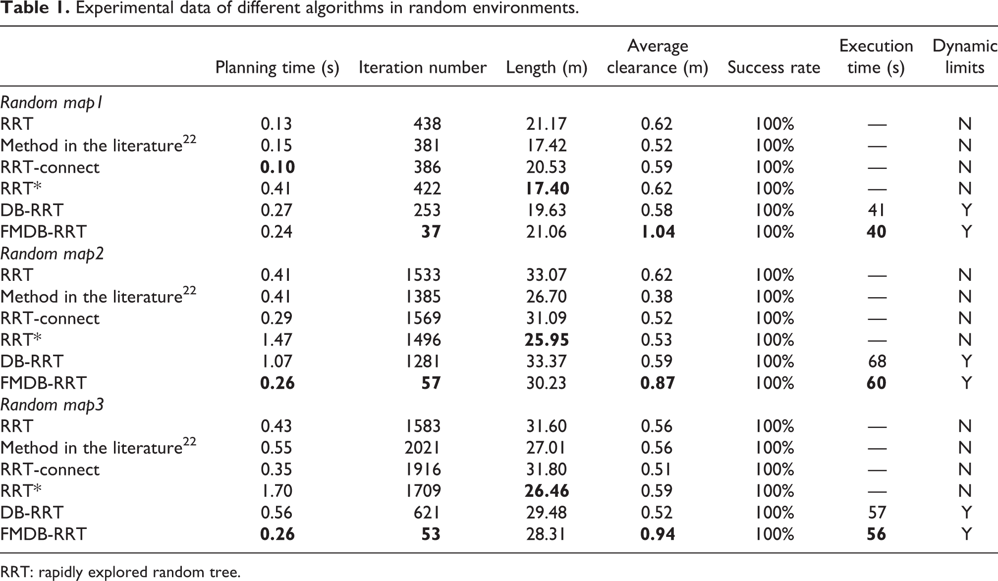
RRT: rapidly explored random tree.

Figure 8.

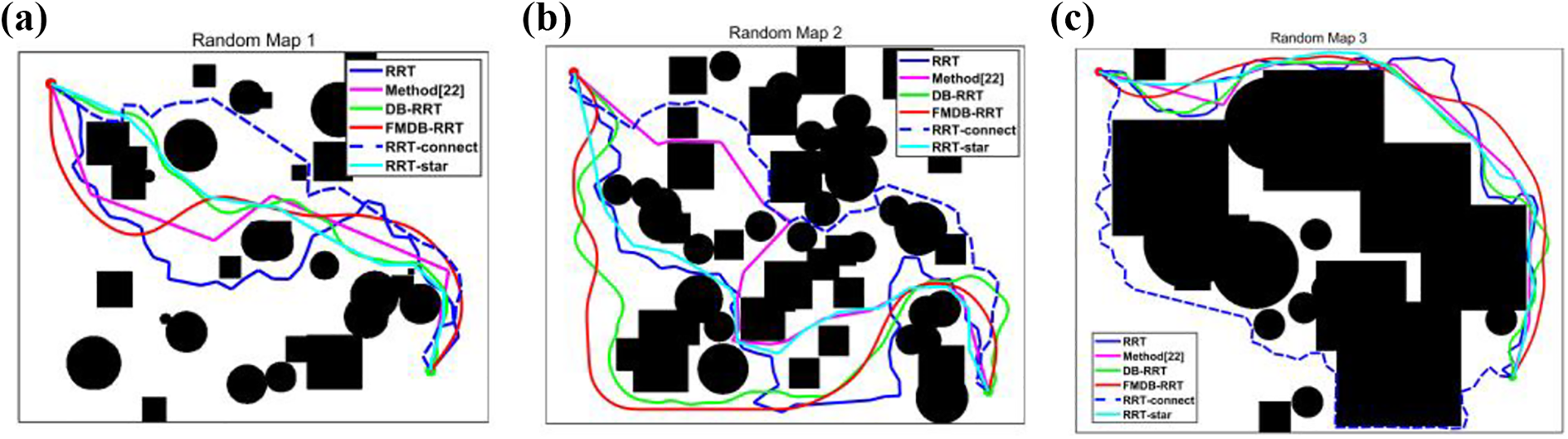
(a–c) Performance of different algorithms in random environments.

Contrasted with the RRT, RRT*, RRT-connect and the method in the literature,²² the proposed DB-RRT algorithm has fewer iterations. RRT* uses some mechanisms such as parent node selection and rewire to generate the shortest path, but it takes a long time. The method in the literature²² has the step of path trimming, it can obtain a shorter path, but the generated path is often too close to the obstacle. The guide path points considering the path curvature are far from obstacles. Therefore, FMDB-RRT can often significantly reduce the number of iterations. The uncertainty of FMDB-RRT is smaller than that of DB-RRT, which reduces the execution time of the trajectory. FMDB-RRT can obtain a higher clearance trajectory, which is safer for the robot that executes this trajectory.

In the environment of random map2 and random map3, FMDB-RRT can obtain shorter planning time through fewer iterations. The DB-RRT algorithm considers the robot’s dynamic constraints, so the planning problem is more complicated than other RRT algorithms that only consider the geometric information. The time of each iteration of DB-RRT is longer than RRT and the method in the literature.²²

As shown in Figure 8, the trajectories obtained by DB-RRT and FMDB-RRT are smoother than other algorithms, and FMDB-RRT has proper clearance. It is worth noting that those trajectories generated by DB-RRT and FMDB-RRT satisfy the dynamical feasibility constraints and can be directly executed by the robot.

Experiments in building environments

The building environment is used to test skilled-RRT and all previous algorithms. At the same time, we also test the FMDB-RRT algorithm with different velocity and acceleration. Table 2 presents the experimental data and the best value in each item is shown in bold. The different performance all algorithms in three building environments is shown in Figure 9. Using the same path guidance, FMDB-RRT trajectories of different accelerations and velocities are too similar, so we draw a trajectory of FMDB-RRT with the maximum acceleration set to 0.4 m/s² and velocity set to 0.5 m/s in the x and y directions.

Table 2.

Experimental data of different algorithms in building environments.

	Planning time (s)	Iteration number	Length (m)	Average clearance (m)	Success rate	Execution time (s)	Dynamic limits	Remark
Factory1
RRT	1.03	2547	47.38	0.47	100%	—	N
Method in the litrerature²²	0.80	2351	39.91	0.36	100%	—	N
RRT-connect	0.60	2520	47.42	0.45	100%	—	N
RRT*	3.86	2562	37.28	0.39	100%	—	N
DB-RRT	2.55	2206	45.72	0.47	100%	91	N
Skilled-RRT	0.47	695	39.74	0.55	100%	—	Partially
FMDB-RRT	0.36	89	47.39	0.92	100%	92	Y
FMDB-RRT	0.40	95	48.47	0.92	100%	98	Y	$a_{max} = 0.3, v_{max} = 0.7$
FMDB-RRT	0.42	147	48.05	0.91	100%	150	Y	$a_{max} = 0.7, v_{max} = 0.3$
FMDB-RRT	0.34	70	47.10	0.92	100%	73	Y	$a_{max} = 0.5, v_{max} = 0.7$
Factory2
RRT	0.56	2388	52.90	0.56	100%	—	N
Method in the literature²²	0.76	2460	42.86	0.49	100%	—	N
RRT-connect	0.51	2801	52.73	0.55	100%	—	N
RRT*	2.22	2411	42.74	0.59	100%	—	N
DB-RRT	1.73	1921	52.00	0.50	100%	101	Y
Skilled-RRT	0.44	711	42.73	0.66	100%	—	Partially
FMDB-RRT	0.33	87	45.61	0.84	100%	90	Y
FMDB-RRT	0.33	91	45.73	0.87	100%	94	Y	$a_{max} = 0.3, v_{max} = 0.7$
FMDB-RRT	0.36	139	45.85	0.83	100%	142	Y	$a_{max} = 0.7, v_{max} = 0.3$
FMDB-RRT	0.28	68	45.46	0.83	100%	71	Y	$a_{max} = 0.5, v_{max} = 0.7$
Office
RRT	1.40	4749	51.54	0.32	100%	—	N
Method in the literature²²	0.84	4081	44.95	0.33	100%	—	N
RRT-connect	0.38	2852	50.26	0.29	100%	—	N
RRT*	4.28	4493	44.03	0.36	91%	—	N
DB-RRT	2.02	1713	48.51	0.36	100%	99	Y
Skilled-RRT	0.43	649	46.44	0.36	100%	—	Partially
FMDB-RRT	0.32	87	45.28	0.52	100%	90	Y
FMDB-RRT	0.32	81	45.85	0.57	100%	84	Y	$a_{max} = 0.3, v_{max} = 0.7$
FMDB-RRT	0.36	143	45.61	0.53	100%	146	Y	$a_{max} = 0.7, v_{max} = 0.3$
FMDB-RRT	0.31	67	45.91	0.51	100%	70	Y	$a_{max} = 0.5, v_{max} = 0.7$

RRT: rapidly explored random tree.

Figure 9.

Performance of different algorithms in building environments. Each column represents the performance of all algorithms in each environment. The third line is an enlarged view of the picture’s green dashed square in the second line.

Similar to the experimental conclusion of “Experiments in random environments” section, FMDB-RRT has better clearance and fewer planning time than other algorithms. DB-RRT has fewer iterations in the nonpath-guided RRT algorithms. Among all the algorithms, only FMDB-RRT and DB-RRT satisfy C² continuity, which is smoother than other algorithms. At the same time, they can generate dynamically feasible trajectories, which robots can directly execute. RRT* still has the shortest path in all environments. RRT-connect has a short planning time in the office environment due to its heuristic growth characteristic.

Both FMDB-RRT and Skilled-RRT are methods that use paths to guide RRT growth. As presented in Table 2, both algorithms have a reasonable success rate. However, FMDB-RRT has fewer iterations, less calculation time, and better clearance. Skilled-RRT following the definition of a small-time controllable system only considers the velocity constraint, but the velocity is not continuous. The noncontinuous velocity causes poor smoothness of the path, see the third row of Figure 9, making Skilled-RRT not applicable to massive robots or vehicles. Furthermore, Skilled-RRT extracts the shortest path on the environment’s skeleton, so the path obtained in a cluttered environment does not have a proper clearance.

In our tests, FMDB-RRT with different velocities and accelerations can generate safer and higher success rate trajectories. When the velocity and acceleration are larger, FMDB-RRT has fewer iterations and shorter planning time.

Experiments on an omnidirectional mobile robot

As FMDB-RRT has smaller uncertainty and higher clearance than DB-RRT, we deploy FMDB-RRT to an omnidirectional robot. To verify the practicability of the algorithm, we set up three different obstacle scenarios in the room of 16.8 × 8.5 m² for the experiment. We use Matlab for trajectory planning and send the planned trajectory to an omnidirectional robot platform for execution. A detailed introduction to the omnidirectional mobile robot platform used in this experiment can be found in the literature.⁴⁰

We use the cartographer⁴¹ for mapping and get an accurate map with a 5 cm resolution. We inflated the map according to the radius of the robot, which is 0.7 m for planning. The calculation of clearance is relative to the inflated map. In this experiment, according to the robot’s physical constraints, the maximum velocity and acceleration in the x and y directions are set to 0.35 m/s and 0.3 m/s², respectively. The remaining parameters are the same as those in the previous experiment.

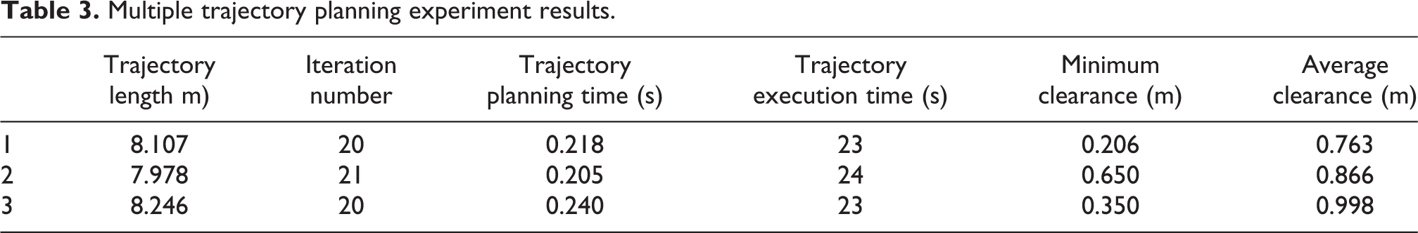
Table 3 presents the experimental data. Figure 10 shows the scene of three experiments. This position of the robot is obtained using the KLD-sampling Monte Carlo localization approach.^42,43 The robot’s position in the environment during the experiment is shown in the right part of Figure 10. In the three experiments, the trajectories obtained by the proposed method have the proper clearance with obstacles. The robot can better track the trajectory obtained by the proposed algorithm.

Table 3.

Multiple trajectory planning experiment results.

	Trajectory length m)	Iteration number	Trajectory planning time (s)	Trajectory execution time (s)	Minimum clearance (m)	Average clearance (m)
1	8.107	20	0.218	23	0.206	0.763
2	7.978	21	0.205	24	0.650	0.866
3	8.246	20	0.240	23	0.350	0.998

Figure 10.

Three experiments in different environments. In the left part, the planned trajectory is represented as the red dotted line. The green line denotes the robot’s actual position when performing the trajectory.

The planned velocity and the actual velocity of the first experiment are shown in Figure 11. The dotted red line denotes the maximum velocity limits. We can see that the planning velocity does not exceed the limit and can be better tracked by the robot. The actual velocities are calculated from the data, which are read from the servo motor’s encoder, and there will be noise because there is no filtering. To sum up, the trajectory generated by our algorithm is smooth and meets dynamical limits, which also have proper clearance with obstacles.

Figure 11.

Comparison of planned velocity and actual velocity.

Conclusion

The proposed DB-RRT method employing the convex hull property of B-spline and the rapid expansion capability of RRT can directly generate a collision-free dynamically feasible trajectory. To further increase the clearance and reduce the randomness of the trajectory, we propose FMDB-RRT.

Comparative experiments show that FMDB-RRT further improves clearance of DB-RRT and reduces planning time. Experiments on an omnidirectional robot indicate that the robot can perform obstacle avoidance smoothly and safely in a clustered environment, verifying the effectiveness of the proposed algorithm.

We plan to expand this work, including extending it to a three-dimensional environment and combining it with a dynamic obstacle prediction module for obstacle avoidance in a dynamic environment.

Footnotes

Declaration of conflicting interests

The author(s) declared no potential conflicts of interest with respect to the research, authorship, and/or publication of this article.

Funding

The author(s) disclosed receipt of the following financial support for the research, authorship, and/or publication of this article: The work was supported by Shandong Key Research and Development Program (Major Science and Technology Innovation Project) [Grant No.2020CXGC010208].

ORCID iD

Chengrui Zhang

Supplemental material

Supplemental material for this article is available online.

References

Sprunk

Lau

Pfaff

. An accurate and efficient navigation system for omnidirectional robots in industrial environments. Auton Robot 2017; 41: 473–493.

Xie

Scheifele

, et al. Heavy-duty omni-directional Mecanum-wheeled robot for autonomous navigation: system development and simulation realization. In: 2015 IEEE International Conference on Mechatronics (ICM), Nagoya, Japan, 6–8 March 2015, pp. 256–261. Piscataway: IEEE.

Paden

Čáp

Yong

, et al. A survey of motion planning and control techniques for self-driving urban vehicles. IEEE Trans Intell Veh 2016; 1: 33–55.

Choset

Hutchinson

Lynch

, et al. Principles of robot motion: theory, algorithms, and implementation. Cambridge, MA: MIT Press, 2005.

Dijkstra

. A note on two problems in connexion with graphs. Numer Math 1959; 1: 269–271.

Hart

Nilsson

Raphael

. A formal basis for the heuristic determination of minimum cost paths. IEEE Trans Syst Sci Cybern 1968; 4: 100–107.

Liu

Atanasov

Mohta

, et al. Search-based motion planning for quadrotors using linear quadratic minimum time control. In: 2017 IEEE/RSJ international conference on intelligent robots and systems (IROS), Vancouver, BC, Canada, 24–28 September 2017, pp. 2872–2879. Piscataway: IEEE.

Pivtoraiko

Knepper

Kelly

. Differentially constrained mobile robot motion planning in state lattices. J Field Robot 2009; 26: 308–333.

Dolgov

Thrun

Montemerlo

. Path planning for autonomous vehicles in unknown semi-structured environments. Int J Robot Res 2010; 29: 485–501.

10.

Oleynikova

Burri

Taylor

, et al. Continuous-time trajectory optimization for online UAV replanning. In: 2016 IEEE/RSJ international conference on intelligent robots and systems (IROS), Daejeon, Korea (South), 9–14 October 2016, pp. 5332–5339. Piscataway: IEEE.

11.

Ratliff

Zucker

Bagnell

, et al. CHOMP: gradient optimization techniques for efficient motion planning. In: 2009 IEEE international conference on robotics and automation, Kobe, Japan, 12–17 May 2009, pp. 489–494. Piscataway: IEEE.

12.

Rösmann

Hoffmann

Bertram

. Integrated online trajectory planning and optimization in distinctive topologies. Robot Auton Syst 2017; 88: 142–153.

13.

LaValle

. Rapidly-exploring random trees: a new tool for path planning. IA, USA: Iowa State University, 1998.

14.

Kuffner

LaValle

. RRT-connect: an efficient approach to single-query path planning. In:. Proceedings of IEEE international conference on robotics and automation, 2000, San Francisco, CA, USA, 24–28 April 2000, pp. 995–1001. Piscataway: IEEE.

15.

Kavraki

Svestka

Overmars

. Probabilistic roadmaps for path planning in high-dimensional configuration spaces. IEEE Trans Robot 1996; 12(4): 566–580.

16.

Moon

Chung

. Kinodynamic planner dual-tree RRT (DT-RRT) for two-wheeled mobile robots using the rapidly exploring random tree. IEEE Trans Ind Electron 2015; 62: 1080–1090.

17.

Karaman

Frazzoli

. Sampling-based algorithms for optimal motion planning. Int J Robot Res 2011; 30: 846–894.

18.

Nasir

Islam

Malik

. RRT*-SMART: a rapid convergence implementation of RRT. Int J Adv Robot Syst 2013; 10: 299.

19.

Qureshi

Ayaz

. Potential functions based sampling heuristic for optimal path planning. Auton Robot 2016; 40: 1079–1093.

20.

Veras

Medeiros

Guimaraes

. Rapidly exploring random tree* with a sampling method based on Sukharev grids and convex vertices of safety hulls of obstacles. Int J Adv Robot Syst 2019; 16: 255798398.

21.

Webb

Van Den Berg

. Kinodynamic RRT*: asymptotically optimal motion planning for robots with linear dynamics. In: 2013 IEEE international conference on robotics and automation, Karlsruhe, Germany, 6–10 May 2013, pp. 5054–5061. Piscataway: IEEE.

22.

Liu

Han

. Dynamic path planning based on an improved RRT algorithm for RoboCup robot. On Robot 2017; 39: 8–15.

23.

Liniger

Domahidi

Morari

. Optimization-based autonomous racing of 1: 43 scale RC cars. Optim Control Appl Methods 2015; 36: 628–647.

24.

Siegwart

Nourbakhsh

Scaramuzza

. Introduction to autonomous mobile robots. Cambridge, MA: MIT Press, 2011.

25.

Brunner

Brüggemann

Schulz

. Hierarchical rough terrain motion planning using an optimal sampling-based method. In: 2013 IEEE international conference on robotics and automation, Karlsruhe, Germany, 6–10 May 2013, pp. 5539–5544. Piscataway: IEEE.

26.

Palmieri

Koenig

Arras

. RRT-based nonholonomic motion planning using any-angle path biasing. In: 2016 IEEE international conference on robotics and automation (ICRA), Stockholm, Sweden, 16–21 May 2016, pp. 2775–2781. Piscataway: IEEE.

27.

Dong

Camci

Kayacan

. Faster RRT-based nonholonomic path planning in 2D building environments using skeleton-constrained path biasing. J Intell Robot Syst 2018; 89: 387–401.

28.

Shan

Dai

Song

, et al. A dynamic RRT path planning algorithm based on B-spline. In: 2009 Second international symposium on computational intelligence and design, Changsha, China, 12–14 December 2009, pp. 25–29. Piscataway: IEEE.

29.

Yoon

Lee

Jung

, et al. Spline-based RRT∗ using piecewise continuous collision-checking algorithm for car-like vehicles. J Intell Robot Syst 2018; 90: 537–549.

30.

Yang

Moon

Yoo

, et al. Spline-based RRT path planner for non-holonomic robots. J Intell Robot Syst 2014; 73: 763–782.

31.

Elbanhawi

Simic

Jazar

. Randomized bidirectional B-Spline parameterization motion planning. IEEE Trans Intell Transp 2015; 17: 406–419.

32.

Alakshendra

Chiddarwar

. Adaptive robust control of Mecanum-wheeled mobile robot with uncertainties. Nonlinear Dynam 2017; 87: 2147–2169.

33.

Yunan

Shuangshuang

Jian

, et al. Research on motion characteristic of omnidirectional robot based on mecanum wheel. In: 2010 International conference on digital manufacturing & automation, Changcha, China, 18–20 December 2010, pp. 237–241. Piscataway: IEEE.

34.

Lynch

Park

. Modern robotics: mechanics, planning, and control. Cambridge: Cambridge University Press, 2017.

35.

Qin

. General matrix representations for B-splines. Vis Comput 2000; 16: 177–186.

36.

Mueller

Hehn

D’Andrea

. A computationally efficient motion primitive for quadrocopter trajectory generation. IEEE Trans Robot 2015; 31: 1294–1310.

37.

Zhou

Gao

Wang

, et al. Robust and efficient quadrotor trajectory generation for fast autonomous flight. IEEE Robot Autom Lett 2019; 4: 3529–3536.

38.

Sethian

. Level set methods and fast marching methods: evolving interfaces in computational geometry, fluid mechanics, computer vision, and materials science. Cambridge: Cambridge University Press, 1999.

39.

Gao

Lin

, et al. Online safe trajectory generation for quadrotors using fast marching method and Bernstein basis polynomial. In: 2018 IEEE international conference on robotics and automation (ICRA), Brisbane, QLD, Australia, 21–25 May 2018, pp. 344–351. Piscataway: IEEE.

40.

Sun

Zhang

Sun

, et al. Safe and smooth motion planning for mecanum-wheeled robot using improved RRT and cubic spline. Arab J Sci Eng 2020; 45(4): 3075–3090.

41.

Hess

Kohler

Rapp

, et al. Real-time loop closure in 2D LIDAR SLAM. In: 2016 IEEE international conference on robotics and automation (ICRA), 2016, Stockholm, Sweden, 16–21 May 2016, pp. 1271–1278. Piscataway: IEEE.

42.

Fox

. Adapting the sample size in particle filters through KLD-sampling. Int J Robot Res 2003; 22: 985–1003.

43.

AMCL. http://wiki.ros.org/amcl. (accessed 7 October 2018).

Supplementary Material

Please find the following supplemental material available below.

For Open Access articles published under a Creative Commons License, all supplemental material carries the same license as the article it is associated with.

For non-Open Access articles published, all supplemental material carries a non-exclusive license, and permission requests for re-use of supplemental material or any part of supplemental material shall be sent directly to the copyright owner as specified in the copyright notice associated with the article.

0.00 MB

Collision-free and dynamically feasible trajectory planning for omnidirectional mobile robots using a novel B-spline based rapidly exploring random tree

Abstract

Keywords

Introduction

Related works

Dynamically feasible B-spline based rapidly random tree

Omnidirectional mobile robot and uniform B-spline

Overview of DB-RRT

Analysis of the sustainable growth of DB-RRT

Quickly determine whether finding a trajectory

Different steer function

SteerToRand function

SteerToGoal function

Guiding the growth of DB-RRT using fast marching

Probabilistic completeness analysis

Lemma 1

Proof

Theorem 1

Proof

Experimental tests

Comparisons and analysis

Introduction to environments and parameters

Experiments in random environments

Experiments in building environments

Experiments on an omnidirectional mobile robot

Conclusion

Footnotes

Declaration of conflicting interests

Funding

ORCID iD

Supplemental material

References

Supplementary Material