Sage Journals: Discover world-class research

Abstract

Current robot polishing techniques are available for objects with computer-aided design geometric models but not for objects without geometric models such as ceramic or clay pots. In this study, we developed a robotic polishing/fettling system to polish the molding defects of ceramic objects. The polishing force on the object surfaces is required to be constant to obtain better results. Thus, the proposed robotic polishing system was designed with a stepper motor, ball screw, and force sensor. The proposed system acquired a rough robot polishing/fettling trajectory and adopted a fuzzy proportional–integral–derivative controller to regulate the trajectory to maintain the desired contact force response from a ceramic object. We developed the temporary desired value technique to make the polishing force response close to the desired one. We validated the system on a six-degrees-of-freedom Staubli TX 40L robotic arm. Experiments were performed to test the effectiveness of the system. The robot trajectory responses showed that the proposed system performed well in tracking the desired force in the polishing/fettling process. We used a 3D microscope to verify that the molding defect of the ceramic pot was significantly removed to evaluate the polishing/fettling quality.

Keywords

Robot polishing/fettling clay pot fuzzy-PID temporary desired value technique

Introduction

In manufacturing industries, the final finishing process to produce high-quality surfaces is known as polishing.¹ Fettling involves converting a crude casting into a quality component by removing undesired material from the surface. In the context of casting, fettling indicates the removal of unwanted edges or material. Fettling is generally performed by highly skilled, experienced workers. However, manual polishing is slow and lacks repeatability and quality control.² In addition, the process is labor intensive and hazardous because of the presence of abrasive particles.³ Hence, manual polishing needs to be urgently replaced with automation.

Previous studies on polishing automation have mainly focused on objects whose polishing trajectories are predefined.⁴ The techniques were not applicable to irregular objects, whose surface geometries were undetermined and varied between products. This makes it difficult to polish irregular objects. Examples of irregular objects are ceramic pots and clay pots. Such objects that are artworks also require fine finishing. Therefore, it is a challenge to design a robotic fettling system to remove the molding defects of irregular objects.

Some studies have been conducted on polishing automation. Oba et al.⁵ used a motion capture system to acquire the motion trajectories of a skilled worker and then replicated them to control the polishing system. The method used for replication was position control. The problem of using a position control strategy on polishing was that the control did not guarantee that the polishing forces would be within the desired range. Slightly high forces may damage delicate objects such as glasses, ceramic pots, or clay products. Thus, it is very important to perform polishing by considering force control.

Nagata et al.⁶ used both position and force control on a serial robotic arm for polishing a polyethylene terephthalate bottle mold. They concluded that understanding the manipulator dynamics for polishing was essential because the same system design could not be used with parallel robotic manipulators. The use of multiple sensors has been suggested for online monitoring of surface roughness while polishing.⁷ A pneumatic actuator is often used as a compliant tool for polishing, where the actuator extension and retraction can be controlled based on the pressure requirement.^3,8 The drawbacks of pneumatic actuators are that they are bulky and require considerable space.

Jin et al. applied a backpropagation neural network with proportional–integral–derivative (PID) control to gasbag polishing to control the force precisely.⁹ As the gasbag was small, this method restricted the tolerance of the polishing tool. If the variation in the polishing surface is large, this tool would not be helpful to perform efficient polishing. Hence, it is also important to design a polishing tool having a large tolerance for polishing surfaces with variations. Similarly, several studies have been conducted to automate the polishing process. For example, some studies adopted multiple sensors to decide polishing endpoints on rotationally symmetric objects.¹⁰

All the above studies heavily depend on CAD/CAM models of object geometries to perform the position and force control of serial/parallel robotic arms for polishing.¹¹ However, these methods are not applicable for unspecified object geometries. We designed a stepper-actuated robotic polishing system using an active force control technique to overcome this problem. The advantage of this system is that it is capable of polishing objects with slightly varying surface geometries. The proposed method using adaptive force control avoids the need for exact robot position control because the designed polishing system adjusts the position to maintain the desired contact force of the tooltip along the given trajectory in accordance with the workpiece surface.

Research objective

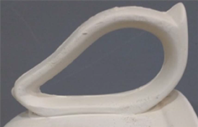
The main objective of this study was to design a robotic polishing system to polish ceramic pots without precise robot trajectories. Figure 1 shows the presence of excess ceramic materials on the handle surface of the ceramic pot to be polished. This polishing process is also called fettling. The polishing tool was required to be mounted on any type of robotic manipulator without knowing the exact robot dynamics, which makes it easier to control robots. Figure 2 shows the flow diagram of the proposed framework for the successful polishing of ceramic or clay objects.

Figure 1.

Polishing/fettling: removal of excess ceramic materials.

Figure 2.

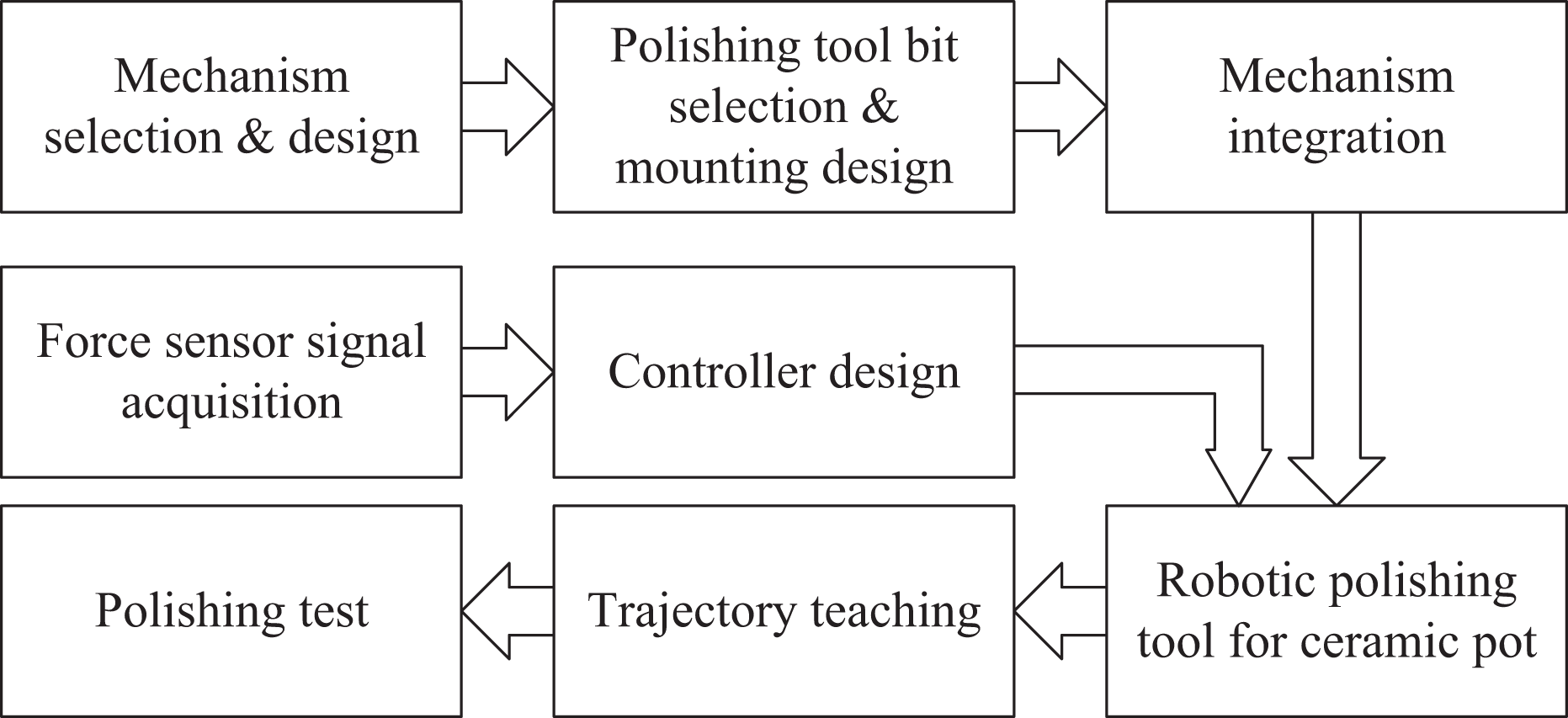
Flow diagram of the proposed framework.

As the polishing tool was designed for any kind of robotic arm, we chose a one-axis polishing mechanism based on a stepper motor. After the actuation mechanism was chosen, several tool bits were tested to perform fettling on ceramic pots manually. The purpose of this process was to choose the most appropriate tool bit for the removal of the defect on the ceramic pot. A direct force control strategy was used in the system. Accordingly, a force sensor was mounted on the robot tip. As the signal from the force sensor contains high-frequency noise, we applied filters to remove the noise. The force sensor detected all the forces acting on it, including the contact force on the tooltip and the gravity of the components and tools attached to the sensor. Force calibration was conducted in this study to remove the gravity effect and other unnecessary external forces. In the polishing process, the object surface geometries were undetermined. The taught robot polishing trajectory was insufficient to achieve good polishing quality. Thus, we applied and tested direct force control using PID and fuzzy PID, respectively. With fuzzy PID, several parameters of the controller were tuned to obtain good force responses. In addition, we developed the temporary desired value (TDV) technique to improve the force response. Finally, the performances of both controllers were validated through several fettling tests using a 3D microscope.

Contributions

A robotic polishing system was proposed for ceramic pots with undetermined surface geometries. We designed a one-axis polishing system compatible with any robotic manipulator. The designed system used a ball screw mechanism actuated by a stepper motor to tolerate the variance in surface geometry.

We proposed a fuzzy PID controller to achieve a better force response than PID control during polishing on ceramic pots. From the results, we observed that the force error in the steady state was within the range of 0.02 N with a force resolution of 0.1 N.

We also proposed the TDV technique to consider the effect of uncertainty in the workpiece surface to improve the force responses.

The remainder of this article is organized as follows. The second section presents a literature review of related work. The third section introduces the proposed robotic polishing system. The fourth section introduces the proposed adaptive-force fuzzy PID controller and the TDV technique. The fifth section presents the experimental results. The sixth section concludes the study.

Literature review of related work

Actuation mechanisms

Gasbag polishing is a type of precision polishing method that uses flexible contact to maintain the force on the polishing surface.⁹ The polishing pressure is analyzed experimentally by the effect of downward depth and inflation pressure, and then, the force model is developed. The gasbag polishing tool was fixed to the robotic arm to realize its motion along the surface of the workpiece. The polishing pressure is dependent on two parameters: downward depth and inflation pressure. The downward depth is controlled by the motion of a six-degrees-of-freedom (6-DOF) robotic arm, and the contact pressure is controlled by the gasbag inflation pressure. A drawback of this polishing mechanism is that the size of the gasbag for polishing is very small, which results in lower tolerance to the variation of the workpiece surface. The robotic arm has to use the position control strategy to obtain the exact trajectory of the polishing surface; hence, it is not suitable for objects with unspecified trajectories. Training the system is very time consuming because a considerable amount of data must be provided to the system for each force value.

Mohammad et al.¹² designed a force-controlled end effector to perform automated polishing using a voice coil motor. The mechanism was used to control the polishing force on the surface. The robotic end effector has a polishing head that can be retracted or extended using a linear hollow voice coil motor (HVCM) actuator. The extension and retraction mechanism was used to apply the desired force on the polishing surface. The force was measured by integrating the force sensor. The HVCM consists of two parts: a magnetic housing and a coil. The magnetic housing is stationary and is fixed to the polishing system, whereas the coil can have linear relative motion with respect to the magnetic housing. Hence, the polishing force can be adjusted by controlling the position of the polishing pad through the HVCM. The voice coil motor does not have a very high resistance value. The HVCM mechanism is suitable for micro-force adjustments, but it cannot be used for high-force applications.

Pneumatic actuation mechanisms are also commonly used in automated polishing processes.^3,8 A pneumatic mechanism uses the concept of a compliant toolhead to control the force on the polishing surface. The tool head is fixed on a pneumatic spindle that can be extended and retracted by pneumatic actuators to provide tool compliance. A pressure sensor and linear encoder can be integrated for feedback control. The movement of the tool over the workpiece is controlled by a parallel robot. In other mechanisms, the links of a parallel robot are controlled by a pneumatic mechanism to exert the desired force on the polishing surface. The system uses an active axial-compliant force device made of three pneumatic cylinders that are constrained to move only in the direction of the tool axis. The pneumatic actuator has the disadvantage of being bulky and occupying considerable space.

Force control

For industrial polishing, it is important to have a robotic system that uses force control to execute the above tasks successfully.^2,12 The motivation behind force control is to provide a robot with better sensing capabilities. These sensing capabilities are important for process automation. Robotic force control makes it easier and safer for humans to work in an industrial unstructured environment. Force control provides a smart manipulation system in unpredictable environments. Force or torque sensors are required to develop a force-controlled system. Most force sensors are developed based on the concept of strain gauges. Typically, the force controller obtains force data from a six-axis force/torque sensor.

In passive force control, the forces are not recorded for feedback control, but they simply adapt to the part so that a constant force is applied. As this technique applies a constant force, it is suitable for applications requiring an almost constant force throughout the process.¹³ Passive control systems consist of pneumatic devices, springs, or mass counterweights. The tool retracts or extracts to trace the part surface. Spring-controlled systems are easy to install in any mechanism because of their linear mechanics. The contact force varies proportionally with deflection according to the spring force constant. Passive compliances are generally of three types: linear (linear deflection), radial (deflection along the radial direction), and rotational (deflection along the arc) compliance systems. Linear compliance allows the tool to deflect along the axial direction with a constant force throughout the entire stroke of the piston. It provides stiffness in the shear direction, which minimizes the chance of shear force damage. Radial compliance allows movement from the axis of the tool to the outward direction. Rotational compliant tools allow deflection at a fixed point along an arc. Similar to linear compliance, this system provides stiffness in the travel direction, but the part must be applied to the tool such that the control force is parallel to the arc of compliance.

Active force control can be divided into indirect and direct force control strategies. Indirect force control does not require closure of the force feedback loop. Impedance control is a common indirect force control strategy.^14
–16 Under impedance control, the robot can be considered a mass spring and damper system whose parameters can be adjusted. In this method, the deviation of the movement of the robotic end effector from its desired movement is related to the contact force. This relationship is given by impedance if the robot control responds to the deviation in motion by generating the corresponding forces. The advantage of indirect force control is that it eliminates the need for external force/torque sensors and improves the robustness and stiffness of the system. However, it has some disadvantages compared with direct force control, that is, impedance control prioritizes motion parameters over force. Consequently, excess forces may be exerted by the end effector on the environment because the controller attempts to maintain the desired dynamic parameters, which can cause harm to the environment.

Direct force control is used to acquire the force value directly using external force or torque sensors. In contrast to indirect force control, direct force control does not require explicit information of dynamic parameters to calculate the force value; instead, it uses the sensor to obtain the force value directly from the interaction with the environment.^17,18 Direct force control uses closed-loop force control. The acquired force is directly used for feedback to formulate the force error value. The force controller mainly uses PID.^9,19 In addition, fuzzy PID control is applied to improve PID control with the help of fuzzy rules.^2,16

The aim of adaptive force control is to stabilize the force in the presence of an unknown robot environment. As indirect force control requires complete knowledge of the environment and the system, direct force control is often used in practice. The objective of adaptive force control is to bring the force error to zero by automatically adjusting the control gains. The advantage of direct force control is that it does not require precise information about the environment. However, it has some limitations. The direct force control law can cause instability in the system, resulting in undesired forces. Hence, the use of damping and signal filtering is crucial to achieve stability.

Factors influencing the removal rate of polishing

It is expected that a larger abrasive particle size results in a higher material removal rate (MRR), and vice versa. In a previous study,²⁰ the authors considered three different polishing conditions for abrasive particle sizes in the range 0–150 nm and observed that the particle size of 80 nm had the maximum MRR. In this study, the results showed that the amount of material removed depended on the projected area of the abrasive particles. However, another study observed that the amount of material removed depended on the volume of abrasive particles rather than just the contact surface area. The polishing pressure or polishing force is one of the most significant factors for quantizing the MRR. The relation between MRR and the polishing pressure can be modeled using Preston’s equation,²¹ where the MRR is proportional to the applied load on the polishing surface and the relative velocity of polishing.

Polishing trajectory acquisition

The robot polishing trajectory can be generated using computer-aided design (CAD)/computer-aided manufacturing (CAM) data.²² The CAD/CAM file of the surface to be polished is imported and used to find the trajectory points for the motion of the robotic end effector or polishing tool. The system follows the trajectory generated by CAD/CAM data using a position and force control system to perform the actual polishing and maintain the contact forces. Also, the trajectory generation algorithm should guarantee a full coverage of the object to be polished.²³ The main limitation of this acquisition method is that it is only available for objects that have CAD files.

Cameras are used to acquire the trajectory points for polishing. They can be used to create trajectories in different ways. One way is to extract features from a polished surface.²⁴ Another way is to record the motion of the tool in the manual polishing process using a camera and replicate it.⁵ The camera was fixed in front to record the polishing tool angles effectively in one plane. Some techniques are based on standard shapes to differentiate between the object and the features to be polished.²⁵

In some cases, for objects such as ceramic and clay pots, the surface trajectories are not well defined, and the small features and edges to be polished cannot be captured by the camera. The features or trajectory for polishing cannot be easily distinguished using image processing. In such cases, the force sensing technique can be used to obtain the trajectory of the polishing surface. A digitization probe is one such application of this concept. In this concept, the robotic end effector is mounted with a force sensor and a polishing tool. The tool moves in the x direction and touches the surface as it moves. When the force sensor receives the signal, it indicates that the tooltip touches the surface. The value of the z coordinate of the tool is recorded. The recorded coordinate values can then be used for further trajectory planning.

Proposed robotic polishing system

In our study, we used a stepper motor for the actuation of our system. The stepper motor rotates the shaft connected to the ball screw mechanism. The stage connected to the linear guide rail moves as the stepper is actuated. The polishing tool and force sensor are attached to this stage. The polishing tool moves as the motor is actuated to control the polishing force on the workpiece. Figure 3 shows the mechanism used in the proposed robotic polishing system. The tool moves over the workpiece surface using a 6-DOF Staubli robotic arm. The stepper motor with the ball screw mechanism has more tolerance to the workpiece variation because of the shaft length. In addition, it can apply high forces on the workpiece and can have higher force resolutions. In addition, a Dyn Pick (WACOH) six-axis capacitive force sensor was used to measure the forces acting on the polishing tool as the feedback signal for the controller in this system.

Figure 3.

Mechanism used in our robotic polishing system.

Actuation mechanism

The linear ball screw mechanism was used as the actuation mechanism in the proposed robotic polishing system. The purpose of the ball screw mechanism was to convert the rotational motion of the motor to translational motion. Figure 4 shows the top view of our mechanism. Table 1 lists the dimensions of the ball screw mechanism.

Figure 4.

(a–c) Linear ball screw mechanism: top view (all dimensions are in mm).

Table 1.

Specifications of ball screw mechanism.

Moving length	100 mm
Screw diameter	16 mm
Accuracy	0.03 mm
Speed	0–100 mm/s
Horizontal load	80 kg
Vertical load	30 kg
Screw pitch	5 mm

We used a NEMA 23 stepper motor as the actuator in our polishing system. The stepper motor rotates and this rotational motion is converted to translational motion using the ball screw mechanism. We used a DM542A stepper driver to control the stepper motor because it is a fully digital stepper driver developed with advanced DSP control algorithms based on the latest motion control technology. It achieved a unique level of system smoothness, providing optimal torque. The stepper driver obtains the digital or pulse width modulation (PWM) pulse series from the controller to change the direction and speed of rotation of the stepper motor. The total moving length of the linear guide rail was 100 mm. A greater moving length of the linear guide rail indicates more tolerance toward polishing surface irregularities and variations. The linear and angular resolutions of our mechanism are as follows: pitch of linear guide: 5 mm, pulses/revolution: 25,600, and 1 pulse = 1 step. Hence, 1 step = 5/25,600 = 0.0002 mm = 0.2 µm resolution. Each revolution corresponds to 360°. Hence, for each step, 1 step = 360/25,600 = 0.014°/step. A higher revolution resolution results in a higher force resolution, and the accuracy of the system is improved. The direction and speed of the stepper motor are controlled separately by two different control loops. The motor uses a PWM signal for actuation. The PWM frequency is the controller output sent to the stepper motor. In the proposed system, the PWM pulse width should be at least 2.5 µs for the system to operate. For the DM542A stepper driver, the pulse width is >2.5 µs and the duty cycle = 0.5. Hence, time period > (2 × 2.5) µs = 5 µs. PWM frequency (f) = 1/(5 × 10 × 10⁻⁶) s = 200,000 Hz. Thus, for a duty cycle of 50%, the PWM operating frequency should be less than 2 × 10⁵ Hz.

Force sensor

A Dyn Pick (WACOH) six-axis capacitive force sensor was used to measure the forces acting on the polishing tool to perform direct force control in the proposed polishing system. This force sensor was mounted on the polishing system to detect the forces acting on the polishing tool during the polishing process. The linearity of this force sensor is 3%, which is the deviation of the actual load value from the measured force output. In the proposed polishing system, several forces such as those from polishing tools, mountings, and force sensor cables act on the force sensor. These force values should be eliminated. Thus, gravity force is calibrated every time the system starts to polish. The overall residual force value is recorded and canceled out from the current force value. In addition, we observe that the original force signal from the sensor has some noise. The removal of noise is very important for obtaining stable output from the system. We employed a Butterworth low-pass filter with a cutoff frequency of 250 Hz, sampling frequency of 1000 Hz, and order of 10 to remove the higher-frequency noise.

Limit switch

In our polishing system, two limit switches were installed at the two ends of the traveling mechanism. These switches were added to ensure the safety of the entire polishing system. If the tool mounting base hits the limit switch, the system is terminated. Figure 5 shows the limit switches mounted in our system.

Figure 5.

Limit switch fixed to the ball screw mechanism.

Rotary polishing tool

Figure 6 shows a suitable polishing tool along with an appropriate polishing bit fixed to the tool mounting. We used a WL-800 grinder rotary polishing tool, which has the maximum and minimum rpm values of 18,000 and 5000, respectively. The polishing bit was made of a cylindrical soft material appropriate for the ceramic used in our experiment.

Figure 6.

WL-800 rotary polishing tool.

Several tests were performed to find a suitable polishing tool for the ceramic pot. Table 2 provides the different polishing tools used in this study. The tests indicated that the rotary polishing tool was not suitable because it leaves polishing marks on the ceramic pot because of the high MRR. Thus, a linear motion tool was built by fixing a sandpaper of grit number 1500 at the base (tool 4). It was observed that this tool did not leave any marks on the surface, and it had a small MRR. Thus, tool 4 was chosen in the proposed polishing/fettling system.

Table 2.

Different polishing tools and their effects.

Tool no.	Tool	Effect
1: Rotary
2: Rotary
3: Rotary
4: Linear

Tooltip trajectory

We used a force sensor to acquire the rough polishing trajectory. Accordingly, the polishing system turned off the force control and commanded the robotic arm to trace the object surface. When the force sensor detected the force, the coordinates of the contacted point were recorded. Similarly, several points were recorded over the surface at different points. The aim was to obtain a rough polishing trajectory over the handle surface. The points were used to regress the curve fitting. Different trajectories were obtained using different orders of polynomials. Figure 7 shows the sixth-order trajectory with an R ² close to 1.

Figure 7.

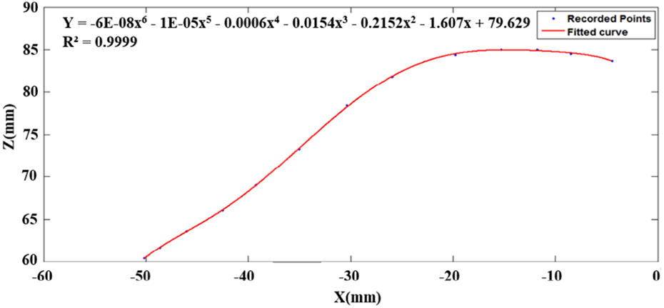
Curve fitting over recorded points with a polynomial of degree 6.

Fuzzy proportional–integral–derivative controller and temporary desired value

System dynamics

It is important to understand all the forces acting on our system to design the controller. The system dynamics will define all the necessary forces acting on the polishing tool and affect the polishing quality. Here, we discuss the forces acting on the polishing tool in the horizontal and vertical directions. Figure 8 shows the forces acting on the polishing tool in the horizontal plane, that is, x–y plane. As the robotic arm moves on the x–y plane, the friction force is generated opposite to the direction of motion. The friction force acting on the polishing bit can be expressed as

F = μ \cdot N

where F is the friction on the polishing bit, μ is the coefficient of kinetic friction, and N is the normal force acting on the polishing surface.

Figure 8.

Forces acting in the horizontal plane.

Figure 9 shows the free body diagram of the polishing tool and polishing surface for the forces in the z direction. By analyzing the forces acting on the polishing surface, we obtain the following. For the polishing surface to be in equilibrium

N - F_{p} = 0.

Figure 9.

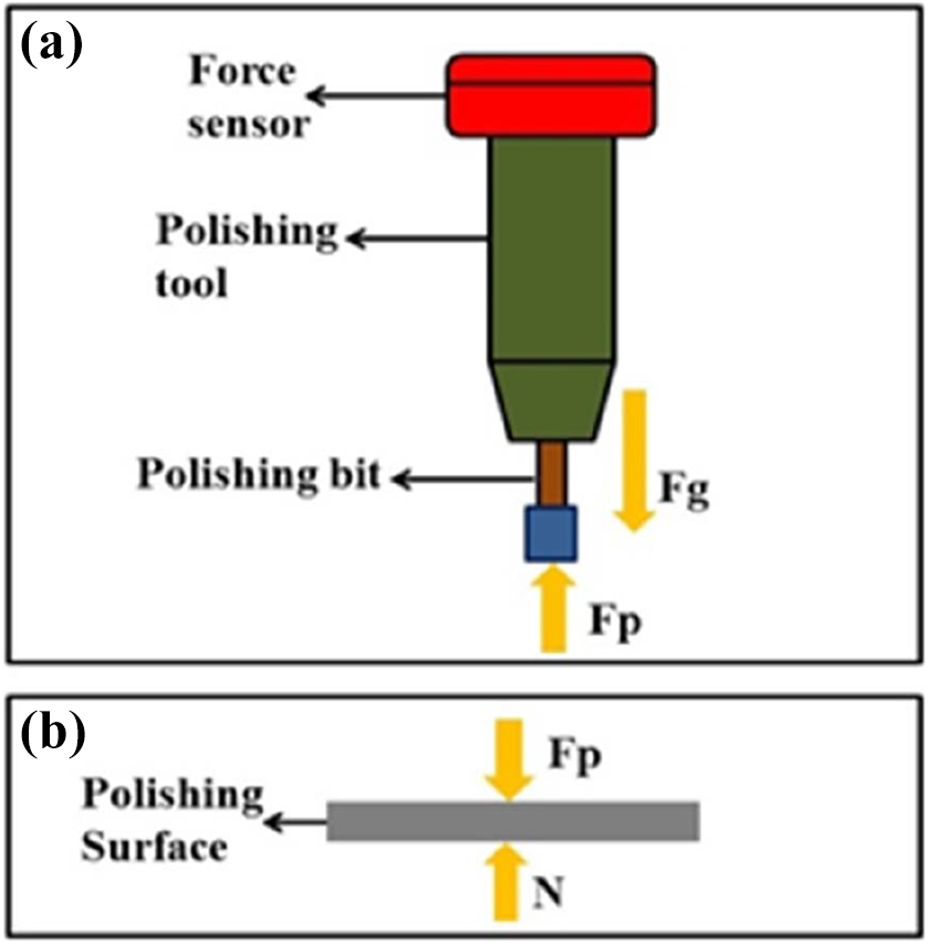
Free body diagram of (a) polishing tool and (b) surface in z direction.

Therefore

F = μ \cdot F_{p}

where Fp is the polishing force acting on the surface.

Apart from the translational friction force, Figure 8 shows that the frictional torque also acts on the polishing bit. The two rotational friction forces reach equilibrium and hence do not provide any resultant force in the direction of motion. The rotational friction generates an opposing torque on the rotating polishing bit. Equations (4) and (5) represent the torque and frictional force acting on the polishing bit, respectively

τ = 2 R \cdot F_{r}

F_{r} = μ \cdot F_{p}

Substituting equation (5) into equation (4), we obtain

τ = 2 R \cdot (μ \cdot F_{p})

where τ is the frictional torque acting on the polishing bit, R is the radius of the polishing bit, and F_r is the friction force due to rotation.

This is the resistant torque that opposes the rotational motion of the polishing tool. The free-body diagram of the polishing tool reveals the forces acting on it in the z direction. These forces can be used to determine the dynamic equations of the polishing tool. From Newton’s law of motion, we obtain

F_{p} - m \cdot g = m \cdot a

Therefore

F_{p} = m (a + g)

where m is the mass of the polishing tool, F_g is the force due to gravity, g is the acceleration due to gravity (9.81 m/s²), and a is the net acceleration in the z direction. The distance traveled in the z direction can be expressed as

Z = \frac{P}{S_{r}} \cdot S

and

a = \ddot{Z}

where Z is the distance traveled in the z direction, P is the pitch of the ball screw (distance traveled in one full rotation of motor shaft), S_r is the number of steps/revolution, and S is the total number of steps moved. Substituting equation (10) into equation (8), we obtain

F_{p} = m (\ddot{Z} + g)

Differentiating equation (9)

\dot{Z} = \frac{d Z}{d t} = \frac{P}{S_{r}} \cdot \frac{d S}{d t}

Since the number of steps moved is equal to the number of PWM pulses

\frac{d S}{d t} = P_{f}

where P_f is the PWM pulse frequency. Substituting equation (13) into equation (12), we obtain

\dot{Z} = \frac{P}{S_{r}} \cdot P_{f}

Differentiating equation (14), we obtain

\ddot{Z} = \frac{P}{S_{r}} \cdot {\dot{P}}_{f}

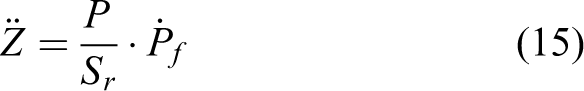
Substituting equation (15) in equation (11), we obtain

F_{p} = m (\frac{P}{S_{r}} \cdot {\dot{P}}_{f} + g)

From the above equations, we observe that the polishing force depends on the rate of change of the PWM pulse frequency. Hence, the polishing force of the system can be controlled by the appropriate change rates of the PWM pulse frequency.

Controller design

Proportional–integral–derivative controller

The governing equation of the PID controller used in our system is defined as

u (t) = K_{p} e (t) + K_{i} \int_{0}^{t} e (τ) d τ + K_{d} \frac{d e (t)}{d t}

where u(t) is the PID output, K_p is the proportional gain, K_i is the integral gain, K_d is the derivative gain, and e(t) is the error at time t.

The PID controller brings the error to zero. Figure 10 shows the PID setpoint set as the desired process variable value. The process variable is then fed to the PID, which provides the output value to actuate the system. However, during the polishing process, some noises and disturbances are introduced to the system. The sensor continues to receive the new process variable value and sends it to PID until the final error value is made close to zero.

Figure 10.

Block diagram of PID controller. PID: proportional–integral–derivative.

K_p , K_i , and K_d are the non-negative coefficients of the P, I, and D components, respectively. K_p is the proportional gain, which accounts for the current error value in the loop. If the error is too large, the PID output will also be large. K_i accumulates all past error values and uses it to generate an output. K_d accounts for the rate of error change. It helps reach the setpoint as soon as possible. Hence, it is very important to tune these coefficients properly to achieve the maximum performance of the system.

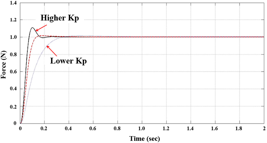
The PID coefficients should be tuned properly to achieve maximum performance. When the PID coefficients are not tuned properly, it will lead to system instability, resulting in force overshoot. The polishing system was modeled under several assumptions to determine system stability; for example, the mass of the polishing system is assumed to be 1 kg. The system was simulated to respond to a unit step input, and the PID controller was implemented to bring the force error to zero and stabilize the polishing system. Figure 11 shows the step input response of the modeled PID controller. While maintaining the integral and derivative parameters constant, we alter the proportional gain to obtain different step input responses. We can observe that as we increase the proportional gain, the system has faster step responses but higher force overshoots. In all the cases, the polishing system brings the error back to zero and stabilizes the system.

Figure 11.

Unit step response of PID-based polishing system. PID: proportional–integral–derivative.

In our system, it is very important for the proposed polishing system to reach the desired force very quickly for polishing a delicate ceramic pot. Hence, considerable force overshoot can damage ceramic pots. In this study, the performance of the controller is evaluated by the effectiveness of the system, such as the settling time to reach the desired value, overshoot, and response time. For a system to have good performance, it should have less overshoot and a short response time to reach the desired equilibrium value. All these parameters are affected by the choice of PID parameters. Under different force values, different sets of PID parameters provide the best performance.

Fuzzy proportional–integral–derivative controller

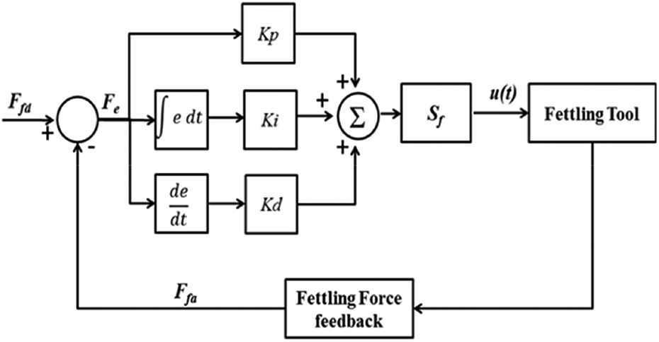
As fuzzy control systems consider human knowledge to design the system output, we designed an adaptive PID control based on fuzzy logic to regulate the PID coefficients. Figure 12 shows the adaptive PID controller. The fuzzy control system consists of three main processes. The first process is fuzzification. This indicates that all the input values are defined into different fuzzy sets using linguistic variables. The fuzzy sets are defined by fuzzy membership functions. Figure 13 shows the membership functions used for the value of the absolute error “e.” The membership functions of “e” had fine divisions for a small range of error to make the system more sensitive to the change in error. Figure 14 shows the membership function for the absolute rate of change of error percentage value. Figure 15 shows the membership functions for K_fp. The next step is the inference engine that defines the rules for each fuzzy membership function using human knowledge to generate the corresponding output. Table 3 provides the rule base for the fuzzy inference system. The next process is defuzzification, which converts the fuzzified output into a crisp value to be used for real applications. The method used for defuzzification is “center of area.” The formula for this method is as follows

COA = \frac{\sum_{i}^{N} μ_{i} x_{i}}{\sum_{i}^{N} μ_{i}}

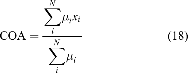
where COA is the value of the center of the area, μ_i is the membership value corresponding to x_i , x_i is the output value, and N is the number of applicable rules. Figure 16 shows the input/output relationship for fuzzy inputs “e” and “rce” and fuzzy output “K_fp.” The surface represents how K_fp varies with the change in “e” and “rce.”

Figure 12.

Block diagram of fuzzy PID controller. PID: proportional–integral–derivative.

Figure 13.

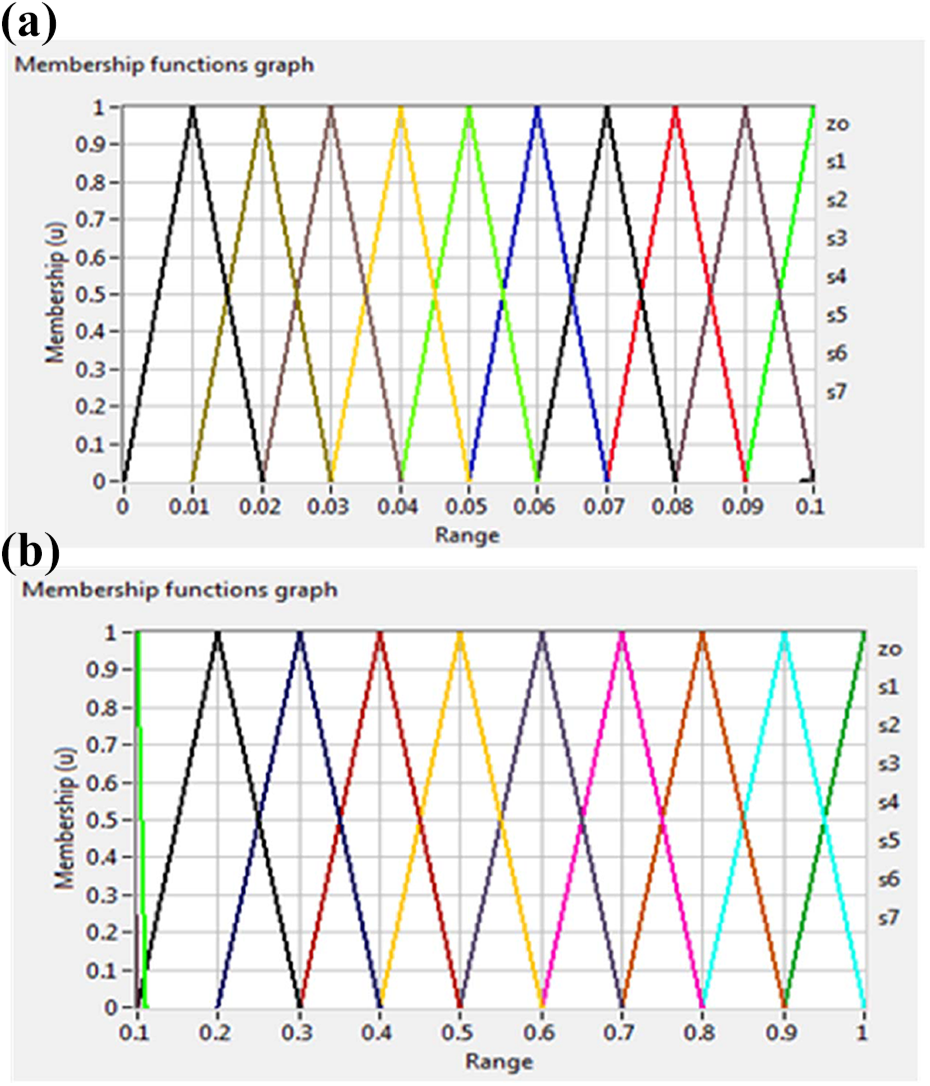
(a) Membership functions for small “e” range (0–0.10). (b) Membership functions for large “e.”

Figure 14.

Membership functions for “rce.”

Figure 15.

(a) Membership functions for a small K_fp range. (b) Membership functions for a large K_fp range.

Table 3.

Rule base of the proposed fuzzy inference system.

	e
rce	ZO	S1	S2	S3	S4	S5	S6	S7	S8	S9
ZO	S	S	S	S	S	S1	S1	S1	S2	S2
S	S	S	S	S	S1	S1	S1	S2	S2	S3
M	S	S	S	S1	S1	S1	S2	S2	S3	S3
L	S	S	S1	S1	S1	S2	S2	S3	S3	M1
VL	S	S1	S1	S1	S2	S2	S3	S3	M1	M1
	e
rce	L1	L2	L3	L4	L5	L6	L7	L8	L9
ZO	S3	S3	M1	M1	M2	M2	L1	L1	L2
S	S3	M1	M1	M2	M2	L1	L1	L2	L2
M	M1	M1	M2	M2	L1	L1	L2	L2	L2
L	M1	M2	M2	L1	L1	L2	L2	L2	L2
VL	M1	M2	L1	L1	L2	L2	L2	L2	L2

Figure 16.

Input/output relationship of the proposed fuzzy system.

After defuzzification, the output crisp value is sent to the controller. We used a fuzzy controller to tune the PID parameters. We performed experiments to test the performance of the fuzzy controller and observed that the system performance is improved. The output from the fuzzy system is used to adapt the PID control. The output from the fuzzy PID controller scales up a constant gain and serves as the input signal for the actuator in terms of frequency. The actual force caused by the actuation is detected by the force sensor and sent back to the controller. The control process repeats until it converges.

Temporary desired value

We propose an innovative TDV technique, which improves the fuzzy PID controller. As the fuzzy controller depends on rule tuning by the user, it is difficult to achieve considerably better results. We developed the TDV technique to enhance the controller response so that it is close to the desired force response to overcome the aforementioned problem. Figure 17 shows the flow diagram of the TDV method.

Figure 17.

Flow diagram of the TDV technique. TDV: temporary desired value.

In most cases, irrespective of how well we tune the fuzzy PID parameters, we cannot achieve the desired response. In our case, because of the uncertainty of the polishing surface, when the controller attempts to achieve the desired force value, the robotic manipulator will need to move to another point on the trajectory, which leads to a poor force response. To overcome this problem, we developed the TDV technique, which generates a temporary desired force response by mirroring the actual response about the desired value in the first polishing pass and used it as the reference for the fuzzy PID controller. The temporary desired force response, to a certain degree, reflects the object surface geometry. As the actual force response is noisy, we applied a moving average filter of 600 points to smoothen the response before mirroring it.

Figure 18(a) shows the force response from the fuzzy PID controller, and Figure 18(b) shows the response after the moving average filter was applied. The filtered actual force response in Figure 18(b) was then mirrored about the desired value of 0.5 N to obtain the temporary desired response. Figure 18(c) shows the response after the TDV.

Figure 18.

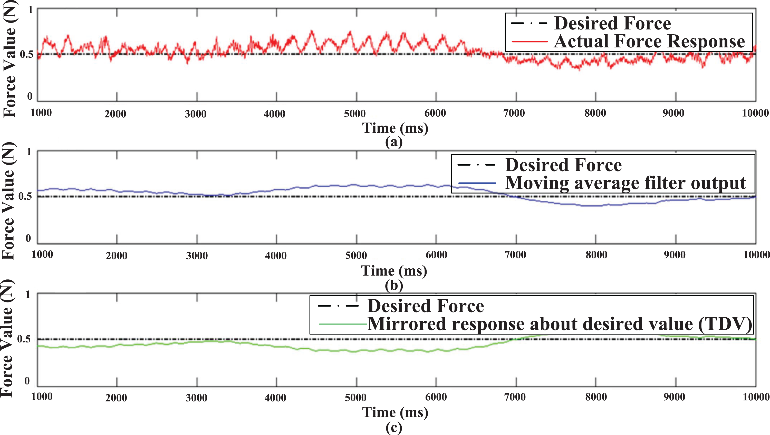
(a) Actual force response from fuzzy PID controller, (b) moving average filter output, and (c) TDV value. PID: proportional–integral–derivative; TDV: temporary desired value.

Figure 19 shows the controller block diagram of the TDV-based fuzzy PID controller. The block diagram shows how the TDV method is integrated into the previously designed fuzzy PID controller. As the TDV represents the workpiece surface geometry in terms of the polishing force response, the TDV method improves the performance of the fuzzy PID controller. In Figure 19, the difference between the desired and TDV responses is regarded as the error, which is used by the fuzzy controller to generate the output gain value. The output from the fuzzy controller is influenced by the controller error and workpiece uncertainty. Subsequently, the fuzzy PID controller continues to use the TDV response for further polishing processing.

Figure 19.

Block diagram of TDV-based fuzzy-PID controller. PID: proportional–integral–derivative; TDV: temporary desired value.

Experimental setup and results

We installed the proposed robotic polishing system to polish a ceramic pot handle, as shown in Figure 20. The ceramic pot was fixed to the pot fixture to confine its motion along all the axes. Figure 3 shows the system setup. We performed several tests to verify the robustness of the system and the efficiency of the designed controller. First, we implemented the polishing system along a taught trajectory without force control. Second, we compared the force responses of the PID and fuzzy PID controllers due to external force disturbances. Third, we investigated the influence of the horizontal velocity of the polishing tool on the force control. Fourth, we investigated the effect of the number of points on the polishing trajectory on the force control. Fifth, as the force control system needs more time to respond to sudden trajectory changes, we also investigated the influence of the order of polynomial curve fitting. Sixth, we evaluated whether the TDV technique helps make the force response close to the actual desired value to improve the performance of the fuzzy PID controller. Finally, we investigated the quality of polishing using a 3D microscope.

Figure 20.

Ceramic pot handle.

Force response without using force controller

Figure 21(a) shows the force response using the fourth-degree curve-fitting trajectory whose R ² was 0.9933. We observed that the force reached the undesired value and passed the threshold of unsuitability for polishing. Figure 21(b) shows the force response using the fifth-degree curve-fitting trajectory, whose R ² was 0.9946. We observed that even though the fifth-degree curve-fitting trajectory was closer to the actual trajectory than the fourth-degree curve, the force response still passed the threshold limits. Figure 21(c) shows the force response using the sixth-degree curve-fitting trajectory with an R ² of 0.9963, which indicated that the trajectory was very close to the actual surface trajectory. The force response indicated that even though the curve-fitting trajectory was regressed very precisely, the forces still exceeded the threshold limits. Thus, the proposed force controller played an important role in the successful polishing process.

Figure 21.

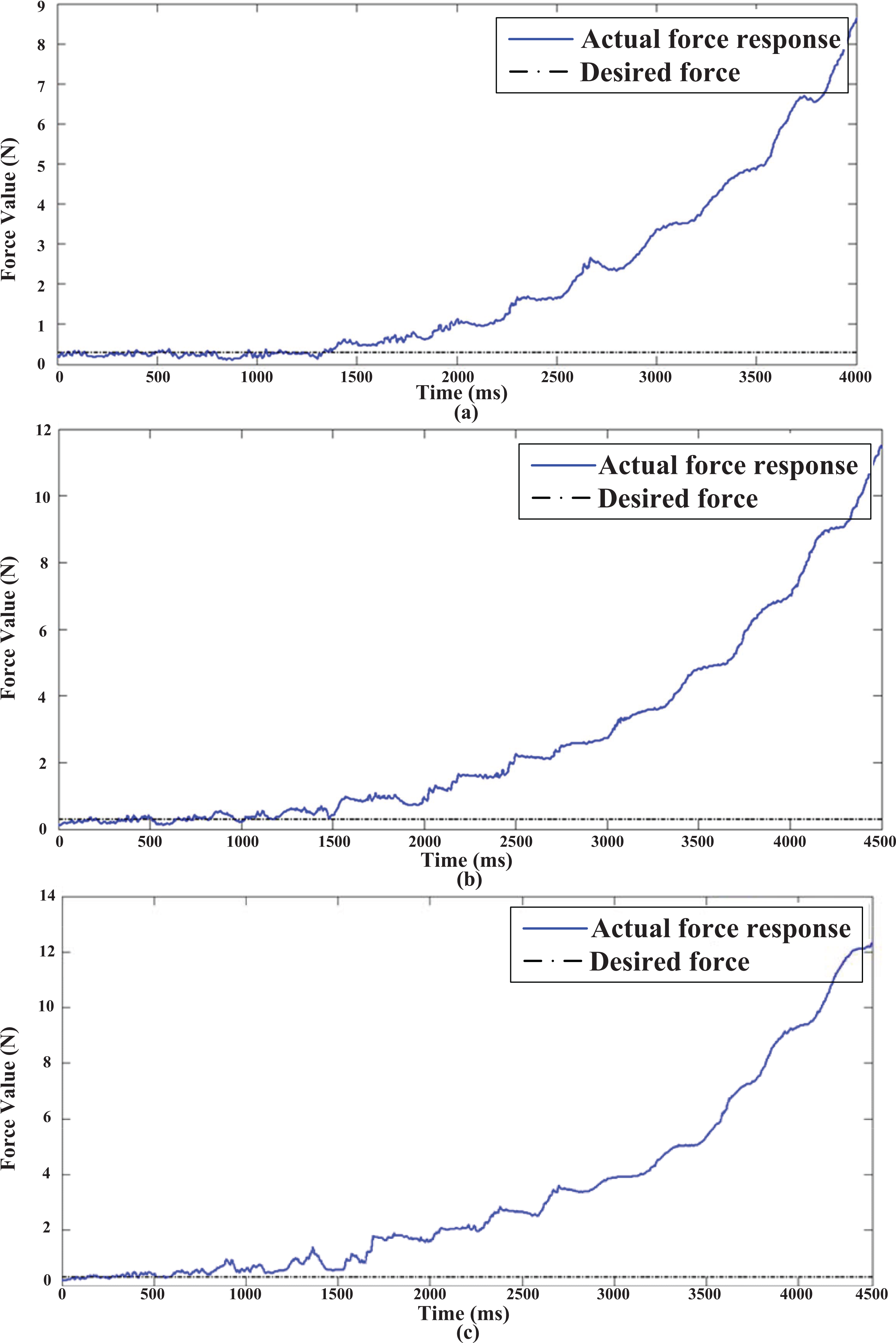
Force response with the (a) fourth-degree, (b) fifth-degree, and (c) sixth-degree curve-fitting trajectory without force control.

Responses of proportional–integral–derivative and fuzzy proportional–integral–derivative controller

We performed experiments using the proposed robotic polishing system to compare the performances of the PID and fuzzy PID controllers. The force response was recorded to validate the performance of the proposed system. Polishing was conducted for two different forces. Figure 22 shows the force response of the PID controller at the desired force of 1.5 N. The force rising time from 0.5 N to 1.5 N was 120 ms without any force overshoot. Figure 22 also shows the force response of the fuzzy PID controller at the desired force of 1.5 N. We observed a rising time of 40 ms with negligible force overshoot. The force reached its desired value quickly without any force fluctuations. After the desired force value was achieved, the system remained stable. Figure 23 shows the force response using the PID controller for a high force of 4 N. The rising time was 80 ms. The force overshoot was 0.3 N. The controller takes some time to maintain a stable force response. The force response oscillated around the desired force. The settling time was 350 ms. Figure 23 also shows the force response of the fuzzy PID controller at the desired force of 4 N. The rising time was 40 ms with an overshoot of 0.2 N. The force became stable quickly. Once the desired force value was achieved, the system remained stable without any fluctuations.

Figure 22.

PID and fuzzy PID force responses at 1.5 N. PID: proportional–integral–derivative.

Figure 23.

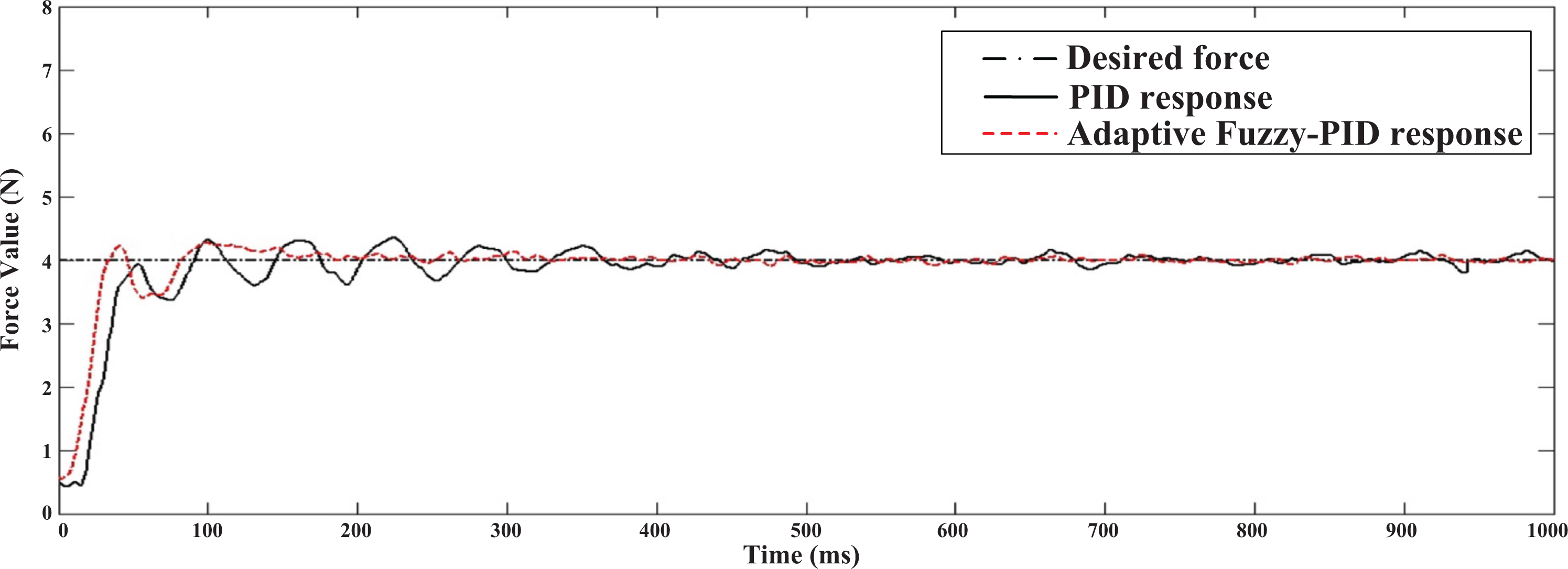
PID and fuzzy PID force responses at 4 N. PID: proportional–integral–derivative.

The second experiment was performed to analyze the system response to an external force disturbance between the PID and fuzzy PID controllers. The force disturbance was introduced manually after the system had already stabilized. Figure 24(a) shows the force disturbance response for the PID controller at a low force value of 1.5 N. It took 200 ms for the PID controller to stabilize the disturbance to the desired force. Figure 24(b) shows that the fuzzy PID controller was also used at 1.5 N and the system took 80 ms to stabilize to the desired force response. The response was steep and quick to nullify the sudden force change. Figure 25(a) shows the force disturbance response of the PID controller at a high force value of 4 N, and the system took 190 ms to stabilize to the desired force response. In Figure 25(b), the fuzzy PID controller was tested at a high force value of 4 N and the system took 75 ms to stabilize. The response was steep and quick. We concluded that irrespective of the operating forces, the fuzzy PID controller provided a quick response to external force disturbance and stabilized it.

Figure 24.

(a) PID controller response to disturbance at 1.5 N. (b) Fuzzy-PID controller response to disturbance at 1.5 N. PID: proportional–integral–derivative.

Figure 25.

(a) PID controller response to disturbance at 4 N. (b) Fuzzy PID controller response to disturbance at 4 N. PID: proportional–integral–derivative.

Force control at different polishing tool movement velocities

The horizontal velocity of the polishing tool affects the polishing force control. The force control required some time to respond to the changing force; however, by the time it responded to the force, the polishing tool moved to a different location, and hence, different forces acted on the polished workpiece. Thus, we evaluated the performance of the proposed controller at different horizontal tool velocities. For example, Figure 20 shows the ceramic pot handle to be polished. As the polishing tool was fixed to the robotic arm, the robotic arm was responsible for the horizontal movement of the tool. Thus, experiments with different horizontal velocities of the robotic arm were evaluated.

The actual polishing was performed at different horizontal velocities on the ceramic pot handle with the tool 4 provided in Table 4. Table 5 provides the force response at different horizontal velocities. The desired force response was 0.5 N. Figure 26 shows the force response for single-pass polishing at three different velocities. We can observe that at any horizontal velocity, the controller brought the force within the desired force range; however, at a lower horizontal velocity, the controller could trace the desired force more accurately. The maximum difference in the mean value from the desired force of 0.5 N was 0.075 N and the maximum standard deviation was 0.2088 N.

Table 4.

Force response at different horizontal velocities.

Velocity (%)	Mean (N)	STD (N)
0.2	0.5755	0.2088
0.1	0.5660	0.1512
0.05	0.5310	0.0892

Table 5.

Force response for different numbers of points on the polishing trajectory.

Number of points	Mean (N)	STD (N)
16	0.5459	0.1406
24	0.5441	0.1202
45	0.5310	0.0892

Figure 26.

Force response at (a) velocity 0.2%, (b) velocity 0.1%, and (c) velocity 0.05%.

Force control for different numbers of points in trajectory

The robotic arm was provided with a rough trajectory to trace the object surface and perform the polishing process. The trajectory was taught by recording the points when the force sensor detected the contact force with the surface. The curve-fitting process was used to generate the trajectory from those points. This trajectory was regressed by several intermediate points. The number of points on the trajectory also affected the quality of the force control.

The ceramic pot handle was evaluated using the sixth-degree curve-fitting method with different numbers of points to evaluate the effect of the number of points on the trajectory on the force control. Table 6 provides the force response when polished using trajectories with different numbers of points on it. The desired force value was 0.5 N. Figure 27 shows the force response of polishing using different numbers of points on the trajectory. If the number of points on the trajectory was small because of the gliding motion, the force value oscillated and then returned when the next point was reached, thus using more points in the trajectory resulted in better force control. The maximum difference in the mean value from the desired force of 0.5 N was 0.045 N and the maximum standard deviation was 0.1406 N.

Table 6.

Force response for different degrees of trajectory curve.

Curve degree	Mean (N)	STD (N)
Fourth	0.5332	0.1047
Fifth	0.5314	0.0987
Sixth	0.5310	0.0892

Figure 27.

Force response for different numbers of trajectory points (N): (a) N = 16, (b) N = 24, and (c) N = 48.

Force control for different degrees of curve fitting

As the degree of curve fitting increased, the quality of curve fitting, R ², increased. The R ² score of the curve fitting affected the polishing result because the force control system required more time to respond to sudden trajectory changes. If the trajectory change was considerable, the system required more time to reach the desired force, but if the trajectory was changed slightly, the system could achieve the desired forces more easily.

Table 6 provides the force response for different degrees of fitted curves. The desired force value was 0.5 N. Figure 28 shows the force response using the trajectories with different degrees of curve fitting. We observed that as the degree of curve fitting increased, the result was closer to the actual surface trajectory because the controller could attain the desired force quickly. The maximum difference in the mean value from the desired force value of 0.5 N was 0.0332 N and the maximum standard deviation was 0.1047 N.

Figure 28.

Force response for different degrees of curve fittings: (a) curve fitting of degree 4, (b) curve fitting of degree 5, and (c) curve fitting of degree 6.

Response with temporary desired value technique

The force response from our controller was successful in tracing the desired force closely, but the response of fuzzy PID depended on the tuning of fuzzy rules, which could vary depending on the users. We used the TDV technique to make the force response close to the actual desired value and to improve the performance of our controller. The performance of the designed technique was compared with the force response without the TDV technique for the results of the curve-fitting trajectories.

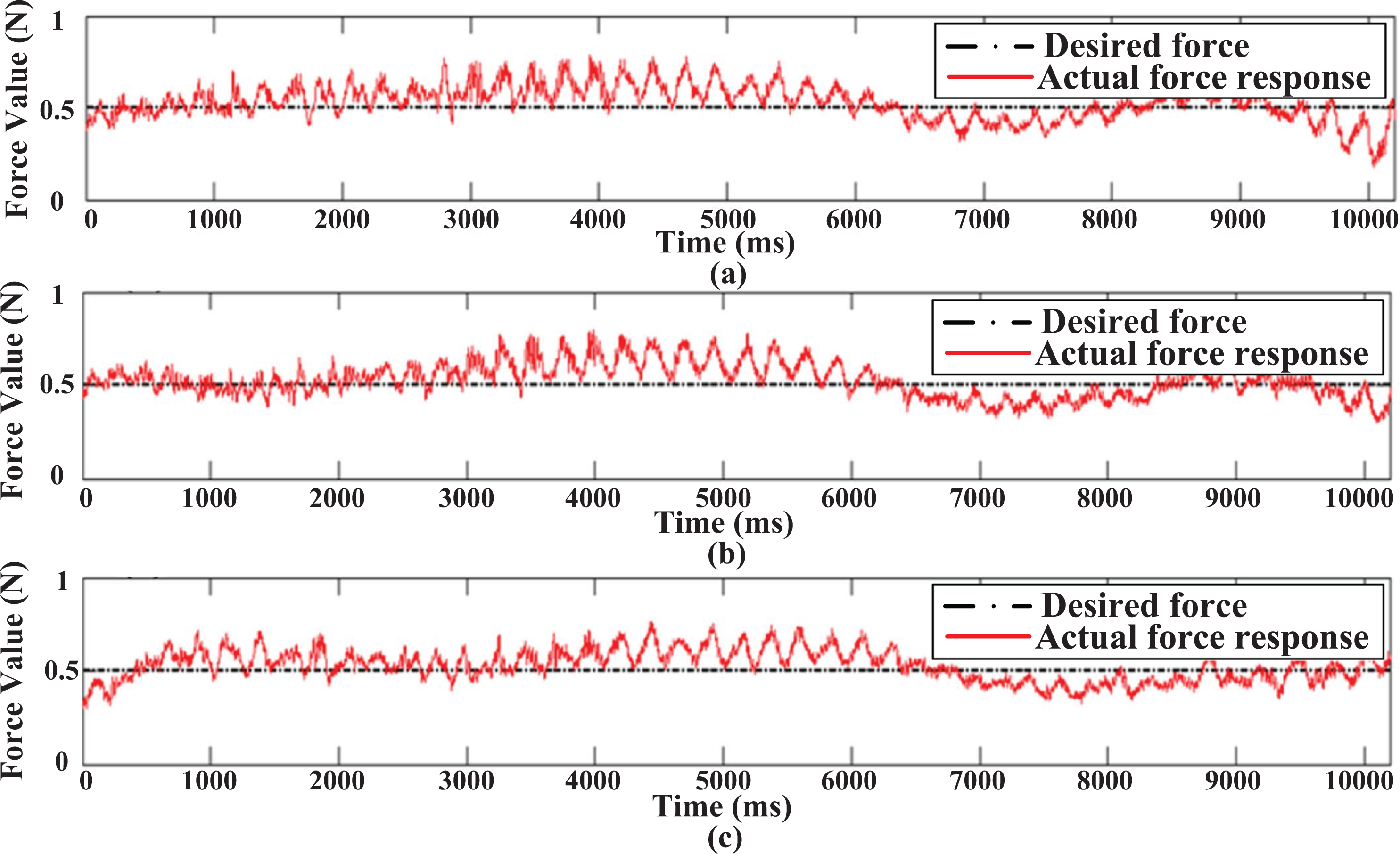
Figure 29 shows the force response of our controller with and without the TDV technique using fourth-degree curve fitting with the desired force of 0.5 N. Figure 29(a) shows the response of the TDV force that was to be traced. The force response without the TDV technique is shown in Figure 29(b). The mean of the force response was 0.5232 N and the standard deviation was 0.1047 N. Figure 29(c) shows the force response using the TDV technique. The force response had a mean of 0.4934 N with a standard deviation of 0.0905 N.

Figure 29.

Polishing force response for degree 4 curve fitting: (a) TDV force response, (b) force response without the TDV technique, and (c) force response with the TDV technique. TDV: temporary desired value.

Figure 30 shows the force response of our controller with and without the TDV technique for polishing using fifth-degree curve fitting with the desired force of 0.5 N. Figure 30(a) shows the value of the TDV force that was to be traced. The force response without the TDV technique is shown in Figure 30(b). The mean of the force response was 0.5214 N and the standard deviation was 0.0987 N. Figure 30(c) shows the force response using the TDV technique. The force response had a mean of 0.4981 N with a standard deviation of 0.0920 N.

Figure 30.

Polishing force response for degree 5 curve fitting: (a) TDV force response, (b) force response without the TDV technique, and (c) force response with the TDV technique. TDV: temporary desired value.

Figure 31 shows the force response of our controller with and without the TDV technique for polishing using sixth-degree curve fitting with the desired force of 0.5 N. Figure 31(a) shows the value of the TDV force that was to be traced. The force response without the TDV technique is shown in Figure 31(b). The mean of the force response was 0.5210 N and the standard deviation was 0.0892 N. Figure 31(c) shows the force response using the TDV technique. The force response had a mean of 0.4977 N with a standard deviation of 0.0845 N. We can observe that the use of the TDV technique makes it possible to trace the desired force more efficiently, irrespective of the degree of the surface trajectory. The force response using the TDV technique is closer to the desired force of 0.5 N. Hence, it can be concluded that the TDV technique improves the performance of the controller.

Figure 31.

Polishing force response for degree 6 curve fitting: (a) TDV force response, (b) force response without the TDV technique, and (c) force response with the TDV technique. TDV: temporary desired value.

Results using Keyence 3D microscope

In the proposed system, fettling was performed using the tool 4 in Table 2. Fettling was performed by 30 back-and-forth passes of the tool 4 at a horizontal velocity of 0.05% over the ceramic pot handle. As the defect size was of micrometer scale, a 3D microscope was used to obtain the size of the defect before and after polishing. Five different points on the pot handle were sampled and examined. The 3D microscope results of these five points before and after polishing are as follows. Figures 32 to 34 show the 3D microscope images of the defect before polishing at points 1, 2, and 3, respectively. The image was captured at a magnification of 12×. The size of the defect was 177.24 µm at point 1, 128.430 µm at point 2, 161.592 µm at point 3, 137.797 µm at point 4, and 234.743 µm at point 5. The mean defect size of the five points was 167.961 µm with a standard deviation of 42.0 µm.

Figure 32.

(a–c) P3D microscope image of the sample before polishing at point 1. Magnification: ×12.

Figure 33.

(a–c) P3D microscope image of the sample before polishing at point 2. Magnification: ×12.

Figure 34.

(a–c) P3D microscope image of the sample before polishing at point 3. Magnification: ×12.

Subsequently, polishing was performed on the ceramic pot handle. The defect size was measured using a 3D microscope at five points as well. The 3D images were captured at a magnification of 12×. Figures 35 to 37 show the 3D microscope images of the ceramic pot handle after polishing at points 1, 2, and 3. The defect size was 0.338 µm at point 1, 0.334 µm at point 2, 3.889 µm at point 3, 0.588 µm at point 4, and 0.337 µm at point 5. The mean size of the five points on the ceramic pot handle after polishing was 1.0972 µm with a standard deviation of 1.564 µm. Compared with the mean size of 167.961 µm and the standard deviation of 42.0 µm before polishing, the defect size was dramatically reduced. The 3D microscope results validated that the proposed robotic polishing system was effective in removing the defects on the ceramic pot. Thus, the proposed robotic polishing system could polish objects with nondeterministic surface geometries well.

Figure 35.

(a–c) 3D microscope image of the sample after polishing at point 1. Magnification: ×12.

Figure 36.

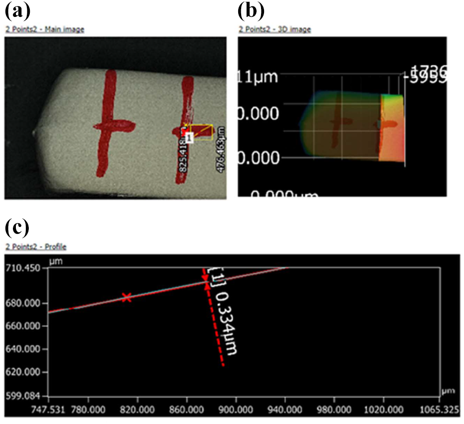
(a–c) 3D microscope image of the sample after polishing at point 2. Magnification: ×12.

Figure 37.

(a–c) 3D microscope image of the sample after polishing at point 3. Magnification: ×12.

Conclusions and future work

In this study, we validated a system for polishing a ceramic pot handle because ceramic pots are fragile and are polished manually nowadays. Position control methods are not suitable for polishing such fragile objects. A force-control scheme is required to achieve good polishing results. Thus, we used adaptive force control in the proposed robotic polishing system. Initially, force control was performed using PID control. The results show that the PID control was not self-sufficient for active force control for polishing applications because of the constant PID coefficients. Subsequently, we applied a fuzzy PID controller in the polishing system. We observed that the fuzzy PID controller outperformed the PID controller because the response was more stable and quicker in nullifying the external force disturbance. However, the force responses were still highly influenced by the polishing trajectory. We observed that the output force response followed a general trend owing to the effect of the workpiece surface. We developed the TDV technique by mirroring the actual response of the desired force in the first polishing pass to obtain a force response closer to the desired force, irrespective of the surface geometry. The temporary desired force response, to a certain degree, represented the object geometry. The results show that the TDV technique can make the actual force response close to the desired one.

The performance of the proposed robotic polishing system was evaluated by conducting various force-response tests. Force control at different polishing tool movement velocities was studied. The proposed polishing system was observed to be effective even at higher velocities. We studied the effect of the number of points on the polishing trajectory on the polishing force response. The results indicated that the robotic polishing system could bring the force response within the threshold limit, even with less information about the workpiece surface. In addition, the results show that using more points on the surface trajectory resulted in a better force response. In addition, several experiments were conducted to determine the force control response at surface trajectories with different curve-fitting orders. The results show that the curve-fitting trajectory with a high degree had a better R ² because it was close to the actual polishing surface trajectory.

We used a 3D microscope to examine the 3D images of the molding defect before and after polishing to validate the proposed system. Before polishing, the mean size of the defect was 167.961 µm with a standard deviation of 42.0 µm; however, after polishing, the mean size of the defect was dramatically reduced to 1.0972 µm with a standard deviation of 1.564 µm. The results demonstrated that the proposed system was effective in performing precise polishing.

The continuously varying environment of a workpiece surface can be simulated to understand the dynamics of the overall system and perform stability analysis. In this study, fettling was performed on a ceramic pot handle. In the future, the fettling process will be widely validated on other parts of a ceramic pot to remove molding defects. The current system requires more iterations of polishing to remove molding defects from the ceramic pot. The parameters influencing the MRR should be optimized to remove the molding defects with fewer iterations of polishing and at higher polishing speeds to accelerate the polishing process.

Supplemental material

Supplemental Material, sj-pdf-1-arx-10.1177_17298814211012851 - Development of robotic polishing/fettling system on ceramic pots

Supplemental Material, sj-pdf-1-arx-10.1177_17298814211012851 for Development of robotic polishing/fettling system on ceramic pots by Zhangguo Yu and Hsien-I Lin in International Journal of Advanced Robotic Systems

Footnotes

Acknowledgement

The authors specially thank Vipul Dubey for his data curation.

Declaration of conflicting interests

The author(s) declared no potential conflicts of interest with respect to the research, authorship, and/or publication of this article.

Funding

The author(s) disclosed receipt of the following financial support for the research, authorship, and/or publication of this article: This work was supported in part by the National Taipei University of Technology, Beijing Institute of Technology Joint Research Program (NTUT-BIT-105-01).

ORCID iD

Hsien-I Lin

Supplemental material

Supplemental material for this article is available online.

References

C-Y

J-R

Liang

Y-J

, et al. Trochoidal toolpath for the pad-polishing of freeform surfaces with global control of material removal distribution. J Manuf Syst 2019; 51: 1–16.

Tian

, et al. Modeling and control of robotic automatic polishing for curved surfaces. CIRP J Manuf Sci Technol 2016; 14: 55–64.

Liao

Liu

. Modeling and control of automated polishing/deburring process using a dual-purpose compliant toolhead. Int J Mach Tools Manuf 2008; 48(12–13): 1454–1463.

Fasbinder

Neiva

. Surface evaluation of polishing techniques for new resilient CAD/CAM restorative materials. J Esthet Restor Dent 2016; 28(1): 56–66.

Oba

Yamada

Igarashi

, et al. Replication of skilled polishing technique with serial–parallel mechanism polishing machine. Precis Eng 2016; 45: 292–300.

Nagata

Hase

Haga

, et al. CAD/CAM-based position/force control for a ball-end abrasive tool and its application to an industrial robot. J Adv Mech Des Syst Manuf 2008; 2(4): 742–752.

Segreto

Karam

Teti

, et al. Cognitive decision making in multiple sensor monitoring of robot assisted polishing. Procedia CIRP 2015; 33: 333–338.

Baran

Plichta

. Grinding and finishing sculptured surfaces using an innovative multitool head with independent pneumatic drive. J Mach Eng 2012; 12: 7–14.

Jin

Pan

, et al. Effect of downward depth and inflation pressure on contact force of gasbag polishing. Precis Eng 2017; 47: 81–89.

10.

Pilný

Bissacco

. Development of on the machine process monitoring and control strategy in robot assisted polishing. CIRP Ann 2015; 64(1): 313–316.

11.

Alao

A-R

Stoll

Song

X-F

, et al. Surface quality of yttria-stabilized tetragonal zirconia polycrystal in CAD/CAM milling, sintering, polishing and sandblasting processes. J Mech Behav Biomed Mater 2017; 65: 102–116.

12.

Mohammad

AEK

Hong

Wang

. Design of a force-controlled end-effector with low-inertia effect for robotic polishing using macro-mini robot approach. Robot Comput-Integ Manuf 2018; 49: 54–65.

13.

Kuo

Y-L

Huang

S-Y

Lan

C-C

. Sensorless force control of automated grinding/deburring using an adjustable force regulation mechanism. In: 2019 international conference on robotics and automation (ICRA), Montreal, QC, Canada, 20–24 May 2019, pp. 9489–9495. New York, US: IEEE.

14.

Blaya

Herr

. Adaptive control of a variable-impedance ankle-foot orthosis to assist drop-foot gait. IEEE Trans Neural Syst Rehabil Eng 2004; 12(1): 24–31.

15.

Zhou

Yue

, et al. Global vision-based impedance control for robotic wall polishing. In 2019 IEEE/RSJ international conference on intelligent robots and systems (IROS), Macau, China, 3–8 November 2019, pp. 6022–6027. New York, US: IEEE.

16.

Chen

Zhao

Yan

, et al. Force control polishing device based on fuzzy adaptive impedance control. In: International conference on intelligent robotics and applications, Shenyang, China, 8–11 August 2019, pp. 181–194. New York, US: Springer.

17.

Huang

Wang

, et al. Design of a flexible polishing force control flange. In: 2016 IEEE workshop on advanced robotics and its social impacts (ARSO), Shanghai, China, 8–10 July 2016, pp. 91–95. New York, US: IEEE.

18.

Chen

Zhao

, et al. Contact force control and vibration suppression in robotic polishing with a smart end effector. Robot Comput-Integ Manuf 2019; 57: 391–403.

19.

Cheng

Qizhi

Lei

, et al. Development of the polishing tool system based on the pneumatic force servo. In: 2017 2nd international conference on advanced robotics and mechatronics (ICARM), Hefei and Taiwan, China, 27–31 August 2017, pp. 126–131. New York, US: IEEE.

20.

Zhou

Shan

Hight

, et al. Influence of colloidal abrasive size on material removal rate and surface finish in sio2 chemical mechanical polishing. Tribol Trans 2002; 45(2): 232–238.

21.

Lee

Jeong

Dornfeld

. Semi-empirical material removal rate distribution model for SiO₂ chemical mechanical polishing (CMP) processes. Precis Eng 2013; 37(2): 483–490.

22.

Stawarczyk

Sener

Trottmann

, et al. Discoloration of manually fabricated resins and industrially fabricated CAD/CAM blocks versus glass-ceramic: effect of storage media, duration, and subsequent polishing. Dent Mater J 2012; 31(3): 377–383.

23.

Rososhansky

. Coverage based tool-path planning for automated polishing using contact mechanics theory. J Manuf Syst 2011; 30(3): 144–153.

24.

Yang

Z-J

Chen

Zhao

, et al. A novel vision localization method of automated micro-polishing robot. J Bionic Eng 2009; 6(1): 46–54.

25.

Hosseininia

Khalili

Emam

. Flexible automation in porcelain edge polishing using machine vision. Procedia Technol 2016; 22: 562–569.

Supplementary Material

Please find the following supplemental material available below.

For Open Access articles published under a Creative Commons License, all supplemental material carries the same license as the article it is associated with.

For non-Open Access articles published, all supplemental material carries a non-exclusive license, and permission requests for re-use of supplemental material or any part of supplemental material shall be sent directly to the copyright owner as specified in the copyright notice associated with the article.

0.00 MB

0.49 MB

	e
rce	ZO	S1	S2	S3	S4	S5	S6	S7	S8	S9
ZO	S	S	S	S	S	S1	S1	S1	S2	S2
S	S	S	S	S	S1	S1	S1	S2	S2	S3
M	S	S	S	S1	S1	S1	S2	S2	S3	S3
L	S	S	S1	S1	S1	S2	S2	S3	S3	M1
VL	S	S1	S1	S1	S2	S2	S3	S3	M1	M1
	e
rce	L1	L2	L3	L4	L5	L6	L7	L8	L9
ZO	S3	S3	M1	M1	M2	M2	L1	L1	L2
S	S3	M1	M1	M2	M2	L1	L1	L2	L2
M	M1	M1	M2	M2	L1	L1	L2	L2	L2
L	M1	M2	M2	L1	L1	L2	L2	L2	L2
VL	M1	M2	L1	L1	L2	L2	L2	L2	L2

	e
rce	ZO	S1	S2	S3	S4	S5	S6	S7	S8	S9
ZO	S	S	S	S	S	S1	S1	S1	S2	S2
S	S	S	S	S	S1	S1	S1	S2	S2	S3
M	S	S	S	S1	S1	S1	S2	S2	S3	S3
L	S	S	S1	S1	S1	S2	S2	S3	S3	M1
VL	S	S1	S1	S1	S2	S2	S3	S3	M1	M1
	e
rce	L1	L2	L3	L4	L5	L6	L7	L8	L9
ZO	S3	S3	M1	M1	M2	M2	L1	L1	L2
S	S3	M1	M1	M2	M2	L1	L1	L2	L2
M	M1	M1	M2	M2	L1	L1	L2	L2	L2
L	M1	M2	M2	L1	L1	L2	L2	L2	L2
VL	M1	M2	L1	L1	L2	L2	L2	L2	L2

	e
rce	ZO	S1	S2	S3	S4	S5	S6	S7	S8	S9
ZO	S	S	S	S	S	S1	S1	S1	S2	S2
S	S	S	S	S	S1	S1	S1	S2	S2	S3
M	S	S	S	S1	S1	S1	S2	S2	S3	S3
L	S	S	S1	S1	S1	S2	S2	S3	S3	M1
VL	S	S1	S1	S1	S2	S2	S3	S3	M1	M1
	e
rce	L1	L2	L3	L4	L5	L6	L7	L8	L9
ZO	S3	S3	M1	M1	M2	M2	L1	L1	L2
S	S3	M1	M1	M2	M2	L1	L1	L2	L2
M	M1	M1	M2	M2	L1	L1	L2	L2	L2
L	M1	M2	M2	L1	L1	L2	L2	L2	L2
VL	M1	M2	L1	L1	L2	L2	L2	L2	L2