Sage Journals: Discover world-class research

Abstract

In this article, an online path planning algorithm for multiple unmanned aerial vehicles (UAVs) has been proposed. The aim is to gather information from target areas (desired regions) while avoiding forbidden regions in a fixed time window starting from the present time. Vehicles should not violate forbidden zones during a mission. Additionally, the significance and reliability of the information collected about a target are assumed to decrease with time. The proposed solution finds each vehicle’s path by solving an optimization problem over a planning horizon while obeying specific rules. The basic structure in our solution is the centralized task assignment problem, and it produces near-optimal solutions. The solution can handle moving, pop-up targets, and UAV loss. It is a complicated optimization problem, and its solution is to be produced in a very short time. To simplify the optimization problem and obtain the solution in nearly real time, we have developed some rules. Among these rules, there is one that involves the kinematic constraints in the construction of paths. There is another which tackles the real-time decision-making problem using heuristics imitating human-like intelligence. Simulations are realized in MATLAB environment. The planning algorithm has been tested on various scenarios, and the results are presented.

Keywords

Path planning UAV assignment problem optimization

Introduction

Path planning problem (PPP) is defined as designing the route of a vehicle, which must follow in such a way that a certain objective is maximized and a goal is reached.¹ In our previous studies, the objective of the PPP was to maximize the collected information from targets in a region of interest (ROI) in a fixed time while avoiding forbidden regions.^2,3 In this study, we generalize our previous studies for online PPPs. It is assumed that the information taken from targets decreases over time (i.e. it becomes out-of-date as time increases). In the literature,⁴ rewards taken from the time-varying reward values of targets are to be maximized. It may be necessary to collect information from the region, where a radio frequency source is located (i.e. detection and tracking)⁵ to cover the maximum area (i.e. search mission),⁶ to overcome uncertainties in the environment,^7,8 and to monitor the slope of the region of the mine.⁹ In the literature,¹⁰ path planning is considered for multiple robots to collect information from an unknown environment. It is aimed that robots collect more information from some regions while avoiding collecting redundant information. In our case, however, the collected information is the captured images from target locations. It is aimed to maximize the collected data from the targets in unit time. There are studies that have designed navigation algorithms for unmanned vehicles for many different purposes. For example, in the literature,^11,12 navigation algorithm is designed to improve the capabilities of an all-terrain unmanned ground vehicle by optimizing its configuration. In the literature,¹³ it is aimed to optimize the data collection utility by jointly optimizing the communication scheduling and trajectory of each UAV. The data collection utility is determined by the amount and value of the collected data. In the literature,⁵ an online path planning algorithm is proposed to detect and track multiple unknown RF targets, but changes in targets with time are not considered.

Moreover, UAVs are not supposed to fly over forbidden zones. In the literature, there are several different solutions to solve the online PPP; a few are utilizing mixed integer linear programming (MILP).^14

–18 A collision-free path planning is realized by continuously adjusting the points defined between the start and goal points.¹⁹ Most of the remaining studies concentrate on the receding horizon control technique to solve the problem.^4,20,21

In this study, the proposed algorithm finds each vehicle’s path by solving an optimization problem over a planning horizon while obeying certain rules. The basic structure in our solution is the centralized task assignment problem, and it produces near-optimal solutions. The solution can handle the case with moving targets, pop-up targets, and UAV loss. It is a complicated optimization problem, and its solution is to be produced in a short time. To simplify the optimization problem and obtain the solution in nearly real time, we have developed many rules. The proposed method ensures that the forbidden zones are not violated, and it works fast enough.

In the literature,^14,15,17,18 where MILP is used, the optimum path from a given starting point till a given ending point is found under vehicle timing and capacity constraints. In the literature,¹⁸ the online PPP is modeled as a multi-UAV task allocation problem by defining the problem as a multitraveling salesmen problem.

In addition to these two approaches, there are approaches based on genetic algorithms (GAs).^22
–24 Unfortunately, these methods are at most quasi-online because of the computational effort required in GA. In the literature,²⁵ they have attacked a similar but slightly modified problem using a rule-based approach.

It is not easy to compare all these approaches’ performance since each study tries to solve a PPP that is different from all the others in constraints or objectives. According to our experience, the critical issue here is how the problem formulation reflects the actual realistic applications. On the other hand, it is always possible to measure each method’s performance over specifically developed scenarios. For example, in the literature,^4,26 exhaustive testing is used to check the performance. As part of their objective, there is the constraint: “every target should be visited only once.” This method for evaluating performance is considered reasonable.

On the other hand, it is not convenient to compare our study with theirs since we do not have such a constraint in our problem definition (on the contrary, targets are expected to be visited repeatedly). As another example, in the literature,^27,28 the results are given for a short mission time. Due to time-varying information values (rewards in their case), re-evaluating the problem after each target visit is not suitable for comparison. Because of these, we have created distinctive scenarios to evaluate our algorithm’s performance, as described in detail in the fifth section.

The main contributions of our study are listed below:

Path planning algorithm has been proposed for environments where the data obtained becomes outdated over time. The proposed method has been shown to produce successful results in cases, where there are moving or pop-up targets. Also, the algorithm has been tested for possible UAV loss situations.

PPP has been converted to a task assignment problem by creating an appropriate objective function. By defining rules which imitate a human path planner, the total amount of “information” is optimized. To the best of our knowledge, this type of study has never been done before in cases where the information gathered changes over time, and variable environmental conditions exist.

The article is organized as follows. The definition of the problem is given in the second section. In the third section, we present the objective function construction. The proposed path planner is introduced in the fourth section. Next, the performance of our path planner is given based on the constructed scenarios in the fifth section. Finally, summary and conclusions and some comments for further studies are shown in the last section.

Problem definition

This study proposes a solution for online PPP for multiple UAVs (N > 1). It is assumed that the UAVs fly at a fixed height. The number of forbidden region (FRs) and desired region (DRs) are M and K, respectively. Since we presume constant-altitude flight, the first step is to define the ROI as a 2D world. We also think that the UAVs sustain a constant speed during the mission. These assumptions are per real-world operational scenarios.²⁹

To define FRs and DRs, we use semialgebraic models.³⁰ Forbidden zones are described using the algebraic primitives of the form

F_{i} = \{(x, y) \in ℝ^{2} | f_{i} (x, y) \leq 0\}, i = 1, \dots, M

(see blue regions in Figure 1) and

f_{i} (x, y) = {(x - x_{i})}^{2} + {(y - y_{i})}^{2} - r_{i}^{2}

Figure 1.

Scenario for online path planning.

where r_i and $(x_{i}, y_{i})$ are the radius and the center coordinate of the i’th forbidden zone, respectively. Thus, we can define the FR as follows

F R = F_{1} \cup F_{2} \cup \dots \cup F_{M}, F R \subseteq ℝ^{2}

In the same way, the definition of the DR can be written as in equations (4) to (6)

D_{j} = \{(x, y) \in ℝ^{2} | g_{j} (x, y) \leq 0\}, j = 1, \dots, K

g_{j} (x, y) = {(x - x_{j})}^{2} + {(y - y_{j})}^{2} - r_{j}^{2}

Here, $(x_{j}, y_{j})$ are the coordinates of the center of the j’th desired zone (target), and r_j is the radius of this zone (Figure 1; the red regions)

D R = D_{1} \cup D_{2} \cup \dots \cup D_{K}, D R \subseteq ℝ^{2}

It is possible to test the algorithm using any other convex shapes; in this case, the algebraic primitives will be changed (i.e. the functions fi (x, y) and g_j (x, y)). Also, we can define nonconvex regions by a combination of convex regions. Having complex areas in the scenario imposes an extra computational burden but does not affect the algorithm’s performance.

UAVs are modeled as Dubins’ vehicles.³¹ Dubin’s vehicle model has been used extensively as a kinematics model in PPP.³² In the literature,³¹ Dubin has shown that the path a vehicle follows always consists of three segments from the list {RSR, RSL, RLR, LRL, LSR, LSL}. R, L, and S denote right turns, left turns, and straight lines, respectively. The problem that is to be underlined is determining the vehicle’s angle for approaching toward targets. The time required to complete the task will increase, and the next choice will be affected due to this crucial detail.

Our study’s focal objective is to maximize the gathered information from DR (i.e. targets). Captured images from targets are considered as gathered information. Besides, it is assumed that the importance of information collected from a target decreases from the time it has been captured if no UAV is flying over the same target. The significance of the images taken from each target decreases with time according to

{CI}_{j} (t) = I_{j} e^{- \frac{t - t_{j l v}}{τ_{j}}}

where ${CI}_{j}$ is the collected information from target j and $τ_{j}, j = 1, \dots, K$ is the time constant for target j. Time constants are the input parameters, and we can use these inputs to define urgencies to some targets (see scenario 5).

Actually, the problem is solved anew at every occurrence of an event (an event is a change in the information as regards the availability of UAVs and completion of the assignment of any target). As already mentioned in our comment, the problem we are supposed to solve is basically an assignment problem. To formulate the problem, we need to construct the “reward (which involves cost implicitly)” matrix. A reward is supposed to decrease with time (we have preferred using exponential decrease associated with a time constant $τ$ ).

The parameter I_t is the information gained when target j is visited at the time $t_{j l v}$ (i.e. the last visited time of target j). Equation (7) indicates that the amount of information gathered from a target becomes out-of-date with respect to time. Hence, each target may be visited several times to maximize instantaneous information.

Naturally, maximizing the instantaneous information gathered can be formulated as an optimization problem based on the expected reward expressed in equation (8)

R I [v_{i}, t_{j}] = max {(I_{j} e^{- \frac{t - t_{j s z} - E T A_{i j}}{τ_{j}}} - α {ETA}_{i j}), 0} j = 1, \dots, K; i = 1, \dots, N

where $t_{j} and, v_{i}$ are target and vehicle indices, respectively. ETA _ij is the expected time of arrival of i’th UAV to j’th target.

The α value is used to adjust the effect of the ETA _ij value in the objective function. When the time constant and I_j value, which are used to calculate the freshness of information, are kept constant in different scenarios, ETA _ij can be very high for targets located at distant positions. In those cases, the ETA _ij value becomes the dominant term in equation (8), which is not desired, as we aim to keep instant information updated. On the other hand, we need to add ETA _ij directly to the objective function for the reasons explained below.

To ensure that ETA _ij value is not dominant in the first term in equation (8), the α value is determined by dividing I_j by the largest ETA _ij value. Thus, it is ensured that the RI values go to zero, not because of the large ETA _ij values. Since we work with fixed targets initially, it is wise to calculate the largest ETA _ij value from the distance between two targets with the maximum distance. We still need to work with pop-up and moving targets later, we use the time to go from one corner to another by following the ROI circumference of the UAV as the largest ETA _ij value.

We calculate the expected time using the waypoints obtained from Dubin’s model by finding Dubin’s paths from each vehicle to each target. This model is prevalent in the literature on UAV motion planning.³² Paths between UAVs and targets are calculated using the following model

{\dot{x}}_{n} = V_{n} cos (Θ_{n} (t)), n = 1, \dots, N

{\dot{y}}_{n} = V_{n} sin (Θ_{n} (t)), n = 1, \dots, N

{\dot{Θ}}_{n} = ω_{n} (t), n = 1, \dots, N

|ω_{n} (t)| \leq \frac{V_{n}}{R_{min}} n = 1, \dots, N

where N is the number of vehicles, $Θ_{n} (t)$ and $V_{n}$ are the heading angle and velocity of n’th UAV, respectively. R _min is the minimum turn radius (13)

R_{min} = \frac{V_{n}^{2}}{tan (Φ) * g}

where $Φ$ is the maximum bank angle for the aircraft and g is the gravitational acceleration.

We want to solve a real-time assignment problem whose solution is strongly dependent on the vehicle entrance angle to targets. As described in the literature,³¹ the desired heading and the vehicle’s desired location must be initialized as an input to the vehicle model. Luckily, we have the initial heading and location of vehicles and the desired locations (i.e. the targets’ centers).

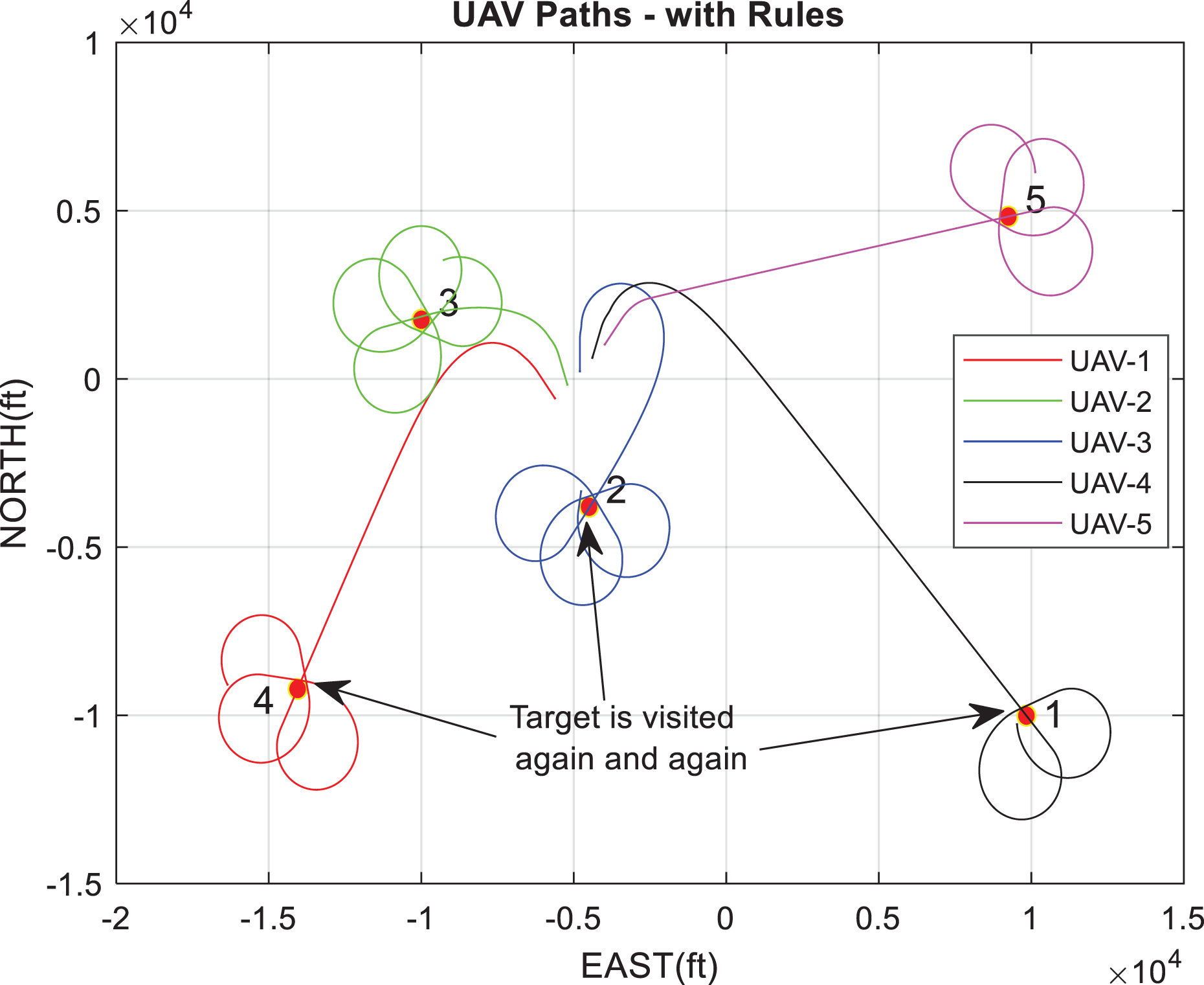
Unfortunately, UAVs’ heading angles at the targets are not known (i.e. they are among the unknowns). We can calculate the distances between centers of target areas and construct the distance matrix at the beginning of a mission. The desired departure angle is determined based on the assignment of the next probable (closest) target. This idea may better be described by investigating Figure 2. For instance, when we calculate Dubin’s path to the sixth goal position, the vehicle’s final heading angle at the end of Dubin’s path will be the angle between North and the line connecting the sixth goal to the 11th position since it is the closest goal to sixth goal position. We can apply this rule only to target regions that are not already assigned to any vehicle. If the 11th position has already been given to a vehicle, then the closest target to the sixth one will be the seventh goal position, which is the second closest position to the sixth (see Figure 2).

Figure 2.

UAV paths to illustrate the critical points in objective function construction. UAV: unmanned aerial vehicle.

Objective function construction

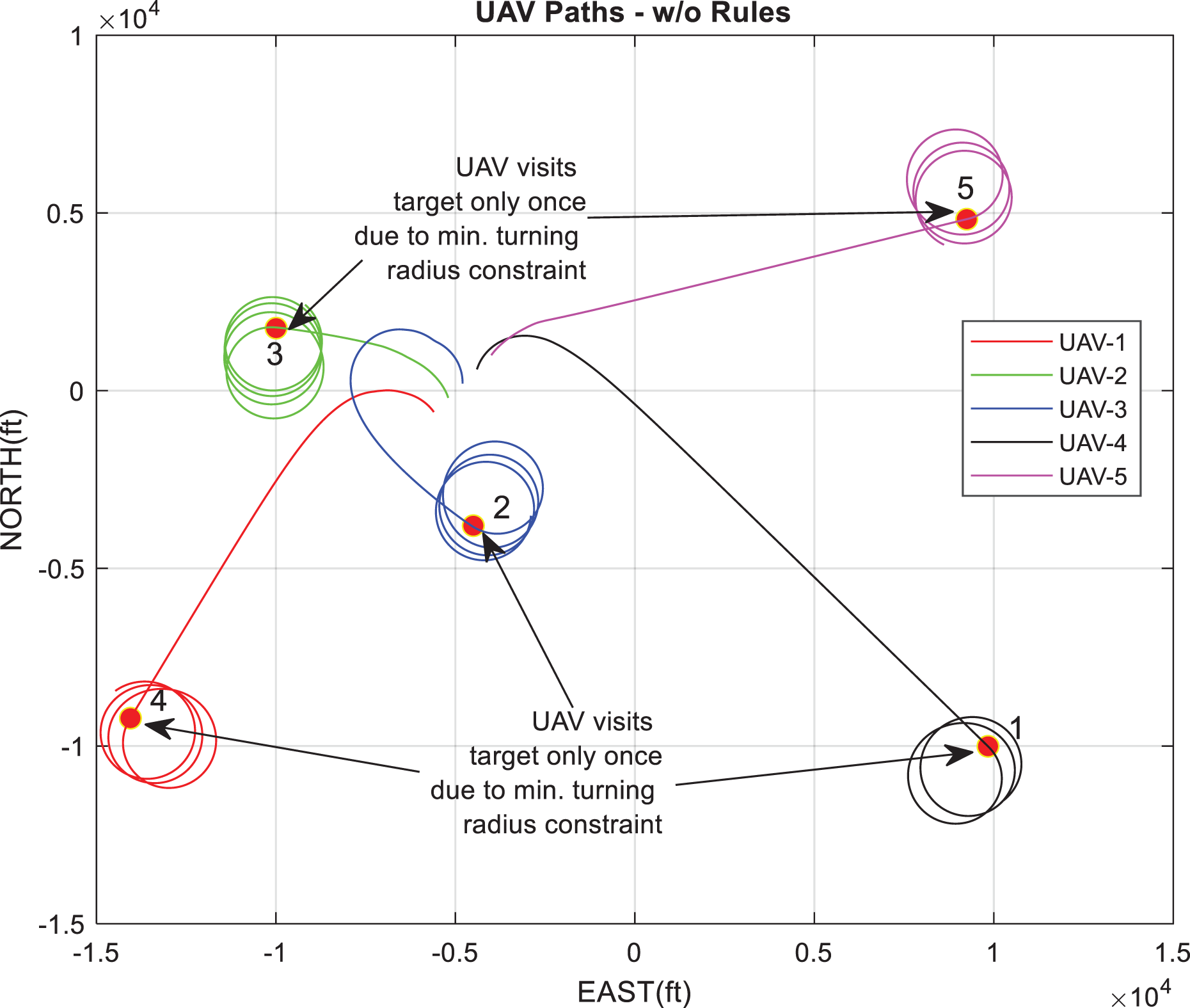
Now, we can express the optimization problem associated with information gathering maximization. But, there are a few critical points to be clarified. We explain them in the following items:

During our studies, it has been witnessed that once a vehicle enters a target, it visits the same target after exiting or it remains inside the same target instead of flying toward other targets (Figure 2, UAV 5). If the j’th target is visited by i’th UAV recently, because the importance level of the information gathered from this target decreases a little, revisiting the j’th target in a short time will make a small contribution to the amount of information. To overcome this situation, we have inserted an extra rule for recently visited targets. The same UAV should not visit target j for a duration of $τ_{j}$ (it is the time that should pass after which it will be worth obtaining a new image from the same target). We adopt this constraint to the problem by setting ETA _ij to an adequately huge value. In our implementation, we have chosen ETA _ij to be equal to max _ij (ETA) (i.e. the reward of visiting the same target is decreased if N ≤ K). In some cases, depending on the entrance or departure angle(s), a UAV cannot enter a specific target due to its kinematic constraints, so information cannot be collected from the target (Figure 10).

Frequently changed assignments for the same vehicle may lead to entirely infeasible paths, as shown in Figure 2 (see UAV 1). To prevent this situation, we append a penalty term to the objective function in the optimization. The following normalization in reward values is made to approach all the vehicles objectively

R I_{norm} = 2 \times \frac{R I [v_{i}, t_{j}] - {min}_{i j} (RI)}{{max}_{i j} (R I) - {min}_{i j} (RI)} - 1

In Figure 2, one can observe all these problems and more simultaneously. In this figure, the assigned goal positions (i.e. targets) are changed mechanically if the ETA is not considered. The first vehicle flies toward to 10th goal position, but, at the instant, the 10th goal position was visited by the fifth vehicle, it turns toward the seventh goal position. This rotation continues with the 16th goal position, 6th goal position, and 11th goal position. Hence, vehicle 1 is in vain to spend time over the white region. The fifth UAV is also incessantly visiting the second goal position and trying to visit the eighth goal position, but it could not, because of the minimum turn radius limitation. It could not escape this vicious circle until the third UAV visits the eighth goal position.

UAVs must not violate FRs, which are defined in equation (3). These can be considered as threats in regions that vehicles function. To avoid forbidden areas, the method used in this study resembles the technique used in the literature.³³ However, we have to find the solution quicker than the manner described in the literature³³ because of timing constraints. The methodology used to do this job is described in detail below. To provide a safety margin around an FR, we define a circle with radius R_i + R _min as the forbidden zone. This circle is divided into pieces of length along which a vehicle can travel in a one-time step (i.e. 1 s). While a vehicle escapes from the forbidden zones, it is needed to avoid a turn in Dubin’s path calculation to pass to a point inside the forbidden zones.

In constructing the distance matrix used in the assignment problem, Euclidean distances between each vehicle to desired locations are calculated. The forbidden region violation is also checked during this calculation, which is completed very fast due to the definition (1). For each point on the Dubin’s path, it is checked whether the point is closer to the center of F_i than R_i $(i = 1, \dots, M)$ . If at least one point is found, there is an FR violation (i.e. F_i is violated). To find a new path without FR violation, we define four new waypoints (Figure 3(a)). In this way, we have decreased the number of possible paths from 6 to 4 in Dubin’s path construction.³¹

Figure 3.

Avoiding from forbidden zones (a) initial configuration, (b) collision-free path (red), (c) zoomed view collision-free path between wp1 and wp2, and (d) zoomed view collision-free path between wp3 and wp4.

Firstly, the waypoints are calculated to move from wp2 to wp3 by traveling on the circle with radius R_i + R _min. It is possible to move from wp2 to wp3 either clockwise or counterclockwise. The bearing having the minimum number of points should be selected. The distance between two consecutive points is the distance that the vehicle can go in one second. Afterward, Dubin’s paths between UAV and wp1 and wp3 and wp4 are found by calculating the approach and departure angles appropriately.

While finding a path between wp1 and wp2, the approach angle is calculated using wp2 and immediately after this point on the circle. The departure angle for the path between wp3 and wp4 is calculated using the same approach. Dubin’s path may include a semicircle (i.e. the distance to a final point may be 2 × R _min) depending on approach and departure angles. Because of this, we left a 4 × R _min distance between wp1 and wp2 and between wp3 and wp4. In this way, we guarantee that there is no FR violation during Dubin’s path generation.

In general, we can describe the assignment problem as follows: There are a number of vehicles and a number of targets. Any vehicle can be assigned to an arbitrary target, associated with a cost that may vary depending on the vehicle-target assignment. It is required to attend to all targets by assigning exactly one vehicle to each target so that the assignment’s total reward is maximized. We have formulated the problem as a linear sum assignment problem (LSAP) using the reward matrix R defined below

R = [R I_{n o r m} (i, j) - P e n a l t y_{_} T e r m s (i, j)] = (r_{i j})

The general LSAP can be modeled for N-agent and K-task by introducing a binary matrix X = (xij) such that³⁴

\begin{array}{l} x_{i j} = {\begin{matrix} 1 if row i is assigned to column j \\ 0 otherwise \end{matrix} \\ max_{i j} \sum_{j = 1}^{K} \sum_{i = 1}^{N} r_{i j} x_{i j} \end{array}

subject to

\sum_{i = 1}^{N} x_{i j} \leq 1 j = 1, 2, \dots, K

\sum_{j = 1}^{K} x_{i j} = 1 i = 1, 2, \dots, N

x_{i j} \in \{0, 1\} j = 1, 2, \dots, K, i = 1, 2, \dots, N

But in our case, N and K do not have to be equal, so we need to use the rectangular form of the LSAP. The algorithms based on exhaustive search have exponential complexity increasing with the number of UAVs.³² For this reason, we need an efficient and fast algorithm to solve this assignment problem. If you have noticed, this is quite similar to the assignment problem formulated in the literature,³⁴ except the constraint K = N is replaced by N ≤ K. This assignment problem can be quickly solved both in a centralized or decentralized way.

Path planner

The solution of the PPP has been obtained by solving the assignment problem given in equations (16) to (19) and by applying basic rules like

Rule 1: Keep the last heading for a while (duration depends on UAV velocity) if the assigned target is the recently visited target.

Rule 2: If there were assignment changes after UAV i was assigned to Target j, look at the “possible” assignment by taking a longer horizon. If the result is “change assignment” for this longer time frame, change it now.

Rule 3: If two UAVs are assigned consecutively three times to the same targets, assign each UAV to one of the targets.

Rule 4: It is not permitted to re-enter the same desired region within a certain duration. Proceed the route with the same heading in this duration.

The total mission time (t _f) is fixed and mission duration [t ₀, t _f] is divided into (T > 0) subintervals [t ₀; t ₁]; [t ₁; t ₂];…; [t_T− ₁; t _f] of 1 s. The solution to the assignment problem must be found within 1 s by considering all UAVs, including those appointed before. In Figure 4, a high-level flow diagram of the proposed solution is presented.

Figure 4.

Flow diagram of the proposed method.

Results and discussions

We tested the performance of the proposed algorithm on several scenarios, starting with relatively modest scenarios. For these scenarios, one can predict optimum routes easily. Afterward, we presented results for more “complex” scenarios to demonstrate the proposed algorithm’s effectiveness.

Scenario 1: Basic scenario.

The aim of this scenario (Figure 5) is whether our algorithm makes decisions similar to a human path planner. There are four targets, two forbidden zones, and two UAVs. The expected solution is “Assign one of the UAVs to the first and second targets and the other UAV to the third and fourth targets.”

Figure 5.

Resultant paths for scenario 1.

It is observed in Figure 4 that the solution is as expected. In Figure 6, you can see the enlarged view of a path traversed more than once. In Figure 7, the total reward/information gained from targets is given. The collected information defined in equation (7) decreases exponentially over time, as seen from the figure. The graph’s peaks indicate when the UAV visits the targets and starts collecting information from the targets. As the information gathered from targets becomes outdated over time, each target needs to be revisited after a while.

Figure 6.

Scenario 1: zoomed into the path of the second UAV. UAV: unmanned aerial vehicle.

Figure 7.

Rewards/information for Figure 4 (scenario 1).

Scenario 2: The effect of more UAVs.

This scenario aims to observe the effects of increasing the number of UAVs. There are four targets, two forbidden zones, and three UAVs (This scenario is similar to scenario 1, except there is one more UAV). The expected solution is “Assign one of the vehicles to the first and second targets and the other vehicles to the third and fourth targets.” There are two possibilities for those assigned to target 3 and target 4. The first possibility is to imitate the situation in scenario 1, and UAVs will visit these targets periodically (Figure 8). In the other opportunity, UAV 2 and UAV 3 will concentrate on target 3 and target 4, respectively (Figure 10, and Figure 11). This modification is the consequence of using rule 3. As expected, the instantaneous collected reward is more extensive when compared to scenario 1 (Figure 12).

Figure 8.

Resultant paths for scenario 2.

Figure 9.

The zoomed view of the path in Figure 8 (scenario 2).

Figure 10.

Resultant paths for scenario 2, rule 3 is applied (scenario 2).

Figure 11.

The zoomed view of the path in Figure 10, rule 3 is applied (scenario 2).

Figure 12.

Rewards/information for Figure 10 (scenario 2).

Scenario 3: The same number of UAVs and targets.

In this scenario, there are five targets and five UAVs. It is expected that each UAV will be assigned to a different target and will stay around it. In Figure 13, we observe an expected output: Each UAV is set a specific target and stays there. Due to the dynamics of vehicles, they cannot continuously take information from their targets. We can solve this situation using rule 1.

Figure 13.

The resultant path for scenario 3, rule 1 is not applied.

It is not permitted to re-enter the same target within a certain duration. Proceed to the route with the same heading angle (rule 4). The result of this rule can be better observed in Figures 14 to 16.

Figure 14.

The total amount of gathered information wrt. Time for scenario 3, rules are not applied.

Figure 15.

Paths of UAVs in scenario 3, rule 1 is applied. UAV: unmanned aerial vehicle.

Figure 16.

The total amount of gathered information wrt. Time for scenario 3, rules are applied.

Scenario 4: More complex regions.

The complexity level of a problem is related to the number of regions (both FRs and DRs), the location of the regions relative to each other, and the number of vehicles used to solve the problem. There is no such study investigating the complexity of the path planning scenario to the best of our knowledge. In the literature,¹⁹ we present a modest way of determining the complexity topologically in the offline PPP. However, it is a relative measure, and it cannot be used in the online case as a performance metric. It might be interesting to examine the complexity of the PPP for future studies.

Although there is no accepted norm for deciding on the complexity level of the problem, it is evident that the PPP presented in Figure 17 is intuitively more complicated than that in Figure 5.

Figure 17.

Paths of four UAVs in scenario 4. UAV: unmanned aerial vehicle.

In this scenario, there are 10 targets, 9 forbidden zones, and 5 UAVs. It is observed that the algorithm performs no different than simple scenarios.

Scenario 5: The effect of time constant.

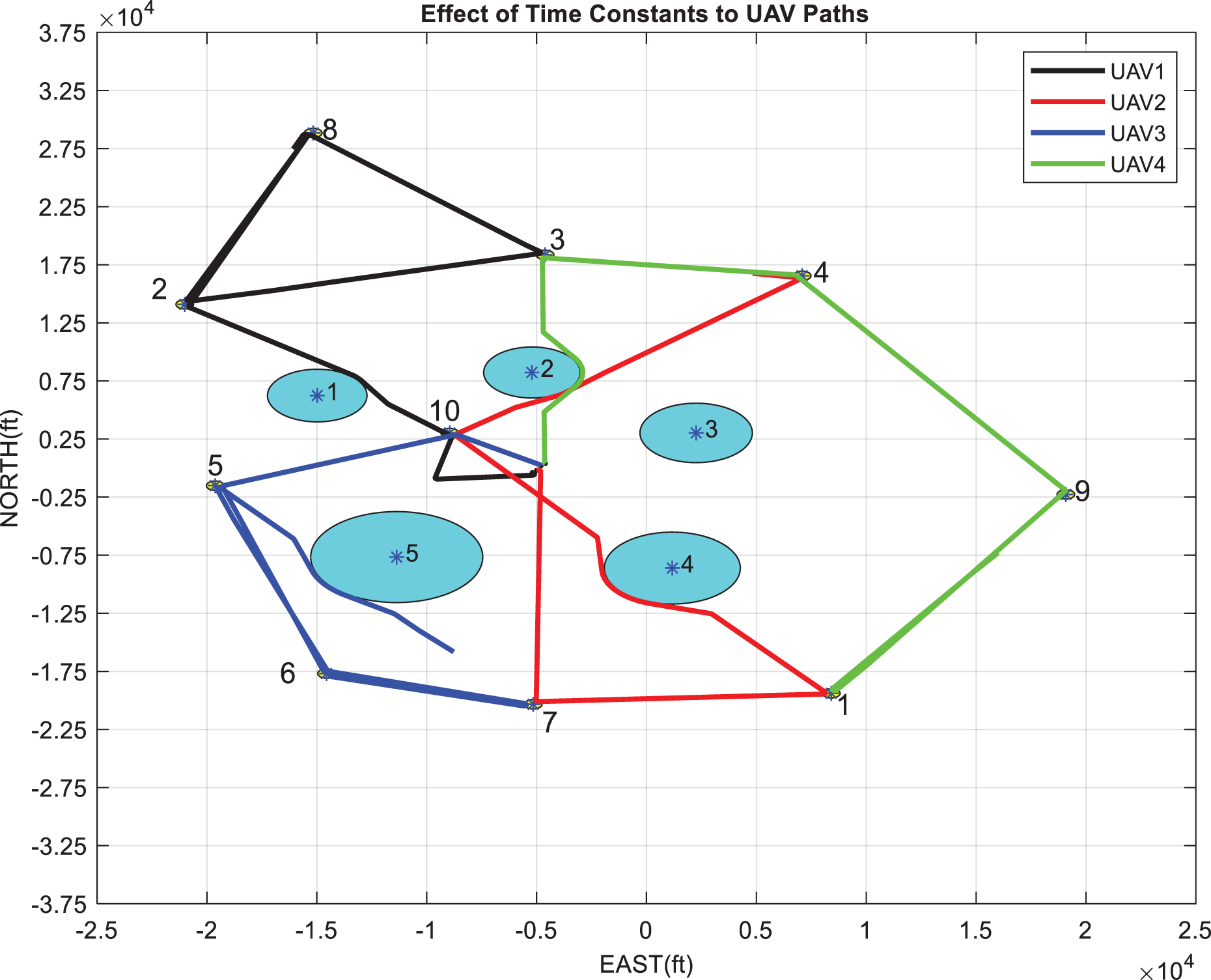
The aim is to observe the effect of the value of the time constant $τ_{j}$ on the resultant paths. In this scenario, there 10 targets, 5 forbidden zones, and 4 UAVs. We have experimented on this scenario by taking $τ_{6} = 100, 70, 55 s$ (the other time constants are fixed at 100 s). The resultant paths are shown respectively in Figures 18 to 20.

Figure 18.

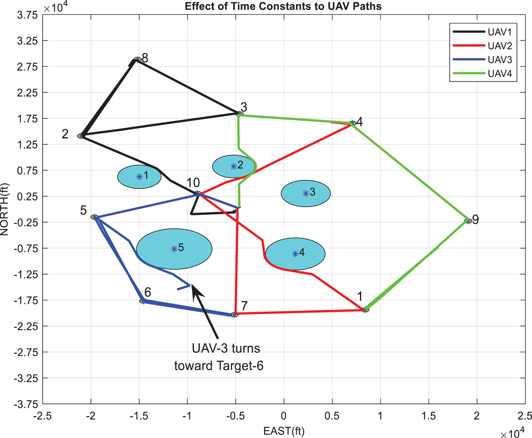
The effect of the time constant (scenario 5): Paths of UAVs for time constants of all targets are the same ( $τ_{i} = 100 s,$ i = 1…10). UAV: unmanned aerial vehicle.

Figure 19.

The effect of the time constant (scenario 5): Paths of UAVs when the time constant of target 6 is decreased to 70 s ( $τ_{6} = 70 s, τ_{i} = 100 s$ for other vehicles). UAV: unmanned aerial vehicle.

Figure 20.

The effect of the time constant (scenario 5): Paths of UAVs when the time constant of target 6 is decreased to 55 s ( $τ_{6} = 55 s, τ_{i} = 100 s$ for other vehicles). UAV: unmanned aerial vehicle.

In Figure 18, UAV 4 goes toward target 7 after visiting target 5. In Figure 19, UAV 4 changes its decision to reach target 7 midway and turns toward target 6. In Figure 20, UAV 4 changes its decision earlier and turns toward target 6.

It can be concluded that the time constant parameters can be used to assign priorities to targets in the objective function construction.

Scenario 6: Moving targets.

Our algorithm can find paths for scenarios having moving targets. In this scenario, we have tested our algorithm using the scenario where moving targets exist. There are five moving targets and one stationary target, four forbidden zones, and three UAVs. It is assumed that the information about these moving targets’ locations is provided by surveillance assets.²⁸

The performance of the algorithm is examined in this kind of scenario with the assumption that targets must not fly over the FRs. The heading angles of moving targets are −90°, −60°, −30°, 0°, 45°, 90° with respect to North, and the speeds of targets are 15, 10, 10, 0, 5, 5 ft/s, respectively. The resultant paths can be observed in Figure 20; the first vehicle (i.e. UAV 1) visits targets 5 and 6, the second one visits targets 1 and 2, and the last one visits targets 3 and 4 in order, as expected intuitively.

If the heading angles of targets are changed to 0°, 70°, −30°, 0°, 45°, −90° with respect to the North, we can see the resultant paths in Figure 21. To observe UAVs’ motion to time, we present their positions at different instants in Figures 22 to 25.

Figure 21.

Paths of UAVs and targets at the end of the scenario 6 (t = 3000 s). UAV: unmanned aerial vehicle.

Figure 22.

Paths of UAVs and targets at the end of the scenario (t = 3000 s) (scenario 7). UAV: unmanned aerial vehicle.

Figure 23.

Paths of UAVs after 500 s (scenario 7). UAV: unmanned aerial vehicle.

Figure 24.

Paths of UAVs after 750 s (scenario 7). UAV: unmanned aerial vehicle.

Figure 25.

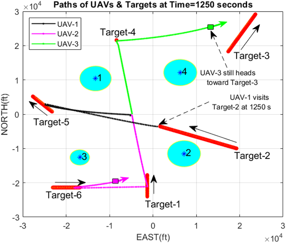
Paths of UAVs after 1000 s (scenario 7). UAV: unmanned aerial vehicle.

Scenario 7: UAV loss.

In this scenario, the problem is investigated for the case in which some of the UAVs are lost during the mission. There are 12 targets, 6 forbidden zones, and 5 UAVs. In Figure 26, we can observe the resultant path when there is no UAV loss. At 1000 s, UAV 2 and UAV 4 are lost. The remaining three UAVs continue the mission. As seen in Figure 27, UAV 1 takes target 1, which was assigned to UAV 2 before its loss, and UAV 5 takes target 2 and target 9, which are assigned to UAV 4 previously.

Figure 26.

Paths of UAVs just before the loss of vehicles (scenario time = 1000 s) (scenario 8). UAV: unmanned aerial vehicle.

Figure 27.

Paths of UAVs after the loss of vehicles (scenario 8). UAV: unmanned aerial vehicle.

Scenario 8: Pop-up targets.

In this scenario, the problem is investigated for the case in which some new targets emerge during the mission. There are six targets at the beginning of the scenario, six forbidden zones, and three UAVs. At t = 1000 s, two new targets are emerged (target 7 and target 8). We can observe the resultant paths before and after the emergence of new targets in Figures 28 and 29, respectively. In Figures 30 and 31, we can observe the instantaneous positions of the UAVs a few seconds before and after pop-up, respectively.

Figure 28.

Scenario 9 without pop-up targets.

Figure 29.

Scenario 9 with pop-up targets, after the pop-up.

Figure 30.

Scenario 9 with pop-up targets, just before pop-up.

Figure 31.

Scenario 9, with pop-up targets, has just appeared.

It is possible to increase the number of scenarios. Due to the page limitations, we have constructed some scenarios just enough to show the most critical issues regarding the performance of our approach.

The algorithm checks new events at every second. Hence, in the worst case, it can be assumed that the problem is solved once at each second (the processing time of scenario with eight UAVs and 20 targets is about 2.5 ms). The worst case computational complexity of the method to solve rectangular form of assignment problem is O(N ³) (see Figure 32). Since the problem is solved anew at every occurrence of an event then the complexity of the presented algorithm is O(VN ³), where V is the number of events. The computational complexity of RI matrix calculation is O(KN). In particular, the simulations were performed in MATLAB and executed on a personal computer, which has the following configuration: 3 GHz processor and 32 GB memory (RAM). The most time consuming part of the algorithm is the assignment problem solution we presented in Figure 32, the processing time versus number of UAVs for the sample scenario having 20 targets.

Figure 32.

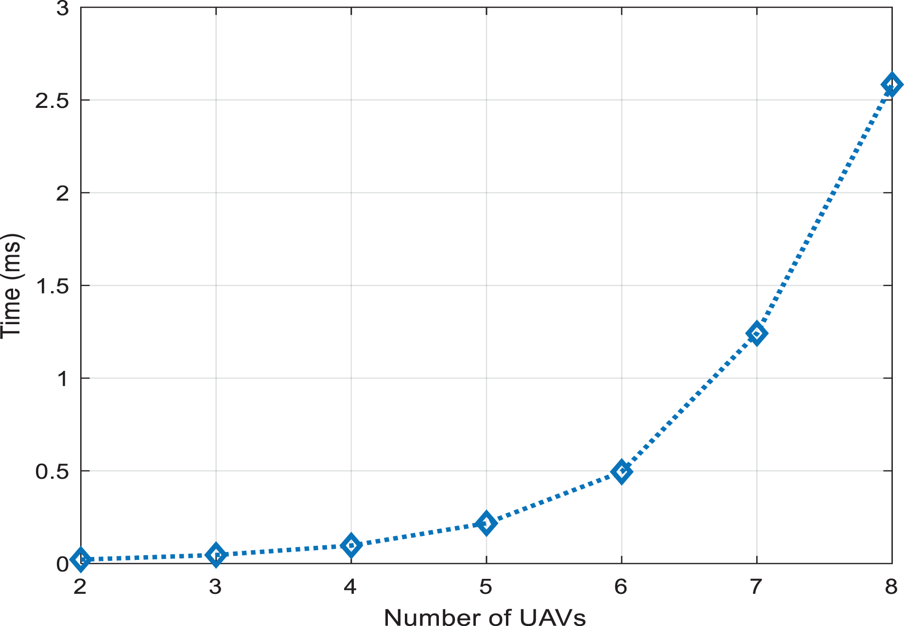
Processing time vs. number of UAVs for the sample scenario having 20 targets.

Investigation of convergence

To examine whether the problem converges or not, we need to examine our algorithm under two main headings: the solution to the assignment problem and the tasks’ status between two consecutive solutions. Frank³⁴ and Burkard et al.³⁵ show that the Kuhn–Munkres algorithm converges to the optimal solution. As we will see from equation (15), the RI matrices we use in the assignment problem take finite values. On the other hand, before the tasks assigned to the vehicles are completed, new tasks can be assigned to the vehicles, or the vehicle may not perform the task due to the kinematic constraints. These problems have already been noted in the manuscript, and they have been taken care of by defining special rules, as given and explained in the fourth section. These rules ensure that vehicles fulfill the tasks. In summary, it can be concluded that the overall algorithm converges a solution.

Conclusions

As indicated before, when the environment is varying, or there is no exact knowledge in advance about the environment, a UAV needs to intelligently plan its path online. Also, in our case, the information taken from targets become outdated. Hence, an online path planner is required to guide multiple UAVs in coordination. We have proposed an online path planning algorithm to guide a group of UAVs to maximize the total amount of information gathered over a given time interval. This centralized algorithm gives acceptable results. As in our offline path planning algorithm,^2,3 some basic rules have been defined to overcome unwanted situations.

In the future, this work can be expanded for the 3D case. In this case, different subproblems such as

3D obstacle avoidance,

fuel consumption (will be useful in making descend or ascend decisions),

if the information obtained is an image, collecting data in different resolutions,

visiting each target at various expeditions at different heights

will need to be included in the problem. Also, in the 3D case of this problem, vehicles’ velocity and altitude should be taken as optimization variables. It may be interesting to find a path for desired locations obstructed by forbidden zones for the 3D case for future studies. If moving targets and their velocities are uncertain, the estimation of the targets’ velocity will be required.

The proposed algorithm need not to be centralized. It could be completely decentralized with the addition of powerful processors on each vehicle. This also requires complete information exchange between the vehicles. In the decentralized case, each vehicle is supposed to run the same algorithm on its own processor based on the information it has. But, while the algorithm is running on a particular vehicle, the available information may change in real time, and the optimum decision of that particular vehicle may be obsolete. Furthermore, there are delays, and sometimes, communication breaks during information exchange. These are very important, of course, not easy to solve problems. We plan to deal with these cases in the future.

Supplemental material

Supplemental Material, sj-docx-1-arx-10.1177_17298814211010379 - Online path planning for unmanned aerial vehicles to maximize instantaneous information

Supplemental Material, sj-docx-1-arx-10.1177_17298814211010379 for Online path planning for unmanned aerial vehicles to maximize instantaneous information by Halit Ergezer and Kemal Leblebicioğlu in International Journal of Advanced Robotic Systems

Supplemental material

Supplemental Material, sj-pdf-1-arx-10.1177_17298814211010379 - Online path planning for unmanned aerial vehicles to maximize instantaneous information

Supplemental Material, sj-pdf-1-arx-10.1177_17298814211010379 for Online path planning for unmanned aerial vehicles to maximize instantaneous information by Halit Ergezer and Kemal Leblebicioğlu in International Journal of Advanced Robotic Systems

Supplemental material

Supplemental Material, sj-pdf-2-arx-10.1177_17298814211010379 - Online path planning for unmanned aerial vehicles to maximize instantaneous information

Supplemental Material, sj-pdf-2-arx-10.1177_17298814211010379 for Online path planning for unmanned aerial vehicles to maximize instantaneous information by Halit Ergezer and Kemal Leblebicioğlu in International Journal of Advanced Robotic Systems

Supplemental material

Supplemental Material, sj-rar-1-arx-10.1177_17298814211010379 - Online path planning for unmanned aerial vehicles to maximize instantaneous information

Supplemental Material, sj-rar-1-arx-10.1177_17298814211010379 for Online path planning for unmanned aerial vehicles to maximize instantaneous information by Halit Ergezer and Kemal Leblebicioğlu in International Journal of Advanced Robotic Systems

Footnotes

Declaration of conflicting interests

The author(s) declared no potential conflicts of interest with respect to the research, authorship, and/or publication of this article.

Funding

The author(s) received no financial support for the research, authorship, and/or publication of this article.

ORCID iD

Halit Ergezer

Supplemental material

Supplemental material for this article is available online.

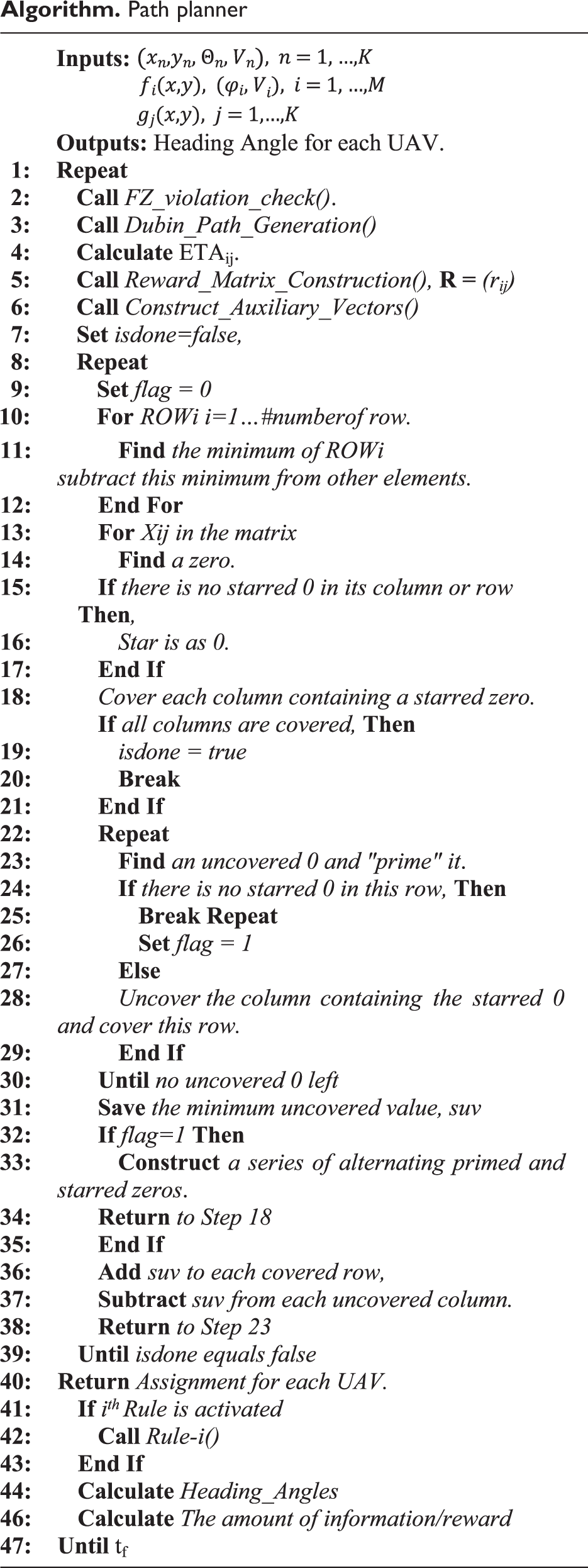
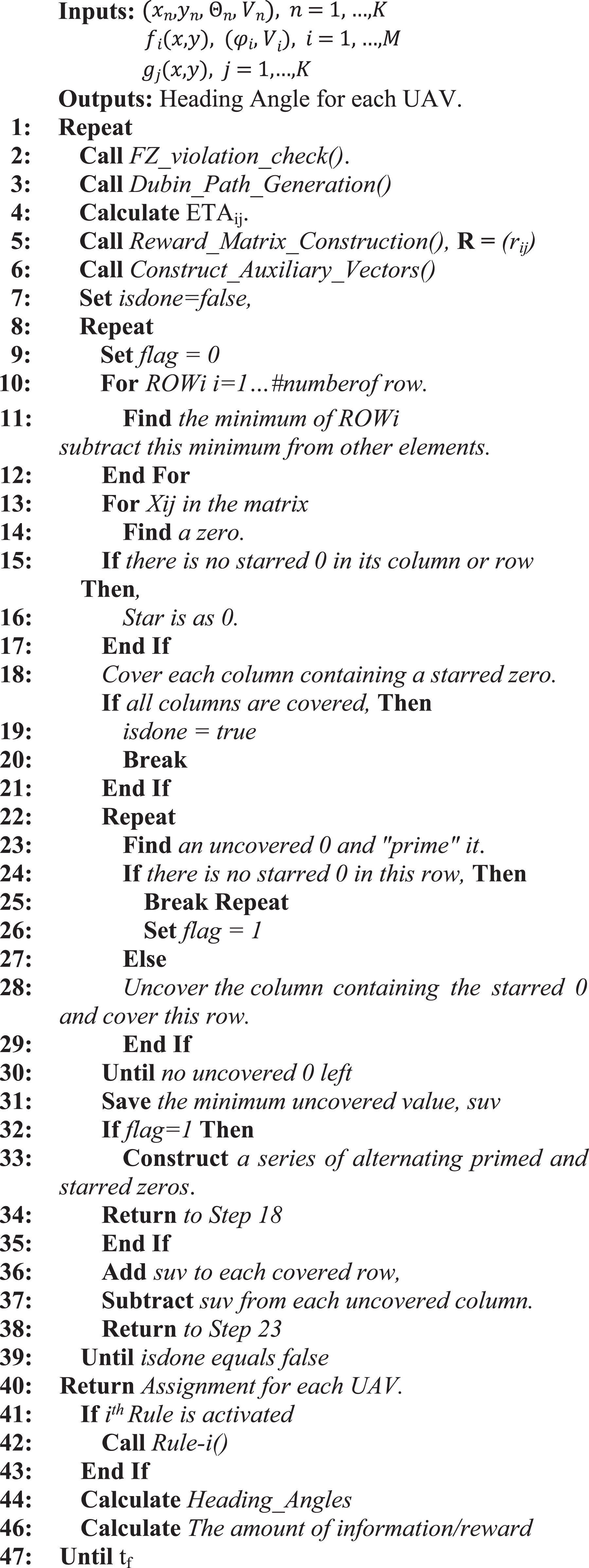
Appendix

Algorithm.

Path planner

References

Otto

Agatz

Campbell

, et al. Optimization approaches for civil applications of unmanned aerial vehicles (UAVs) or aerial drones: a survey. Networks 2018; 72: 411–458.

Ergezer

Leblebicioğlu

. Path planning for UAVs for maximum information collection using evolutionary computation. IEEE Trans Aerosp Electr Syst 2013; 49(1): 502–520.

Ergezer

Leblebicioğlu

. 3D path planning for UAVs for maximum information collection. J Intell Robot Syst 2014; 73: 737–762.

Cassandras

. A cooperative receding horizon controller for multivehicle uncertain environments. IEEE Trans Autom Control 2006; 51(2): 242–257.

Nguyen

Rezatofighi

B-N

, et al. Online UAV path planning for joint detection and tracking of multiple radio-tagged objects. IEEE Trans Signal Process 2019; 67(20): 5365–5379.

Semiz

Polat

. Solving the area coverage problem with UAVs: a vehicle routing with time windows variation. Robot Autonom Syst 2020; 126: 103435.

González-Sieira

Cores

Mucientes

, et al. Autonomous navigation for UAVs managing motion and sensing uncertainty. Robot Autonom Syst 2020; 126: 103455.

Patle

Pandey

Jagadeesh

, et al. Path planning in uncertain environment by using firefly algorithm. Def Technol 2018; 14: 691–701.

Min

Chen

, et al. Computer vision-based techniques and path planning strategy in a slope monitoring system using unmanned aerial vehicle. Int J Adv Robot Syst 2020; 17: 1–14.

10.

Dutta

Bhattacharya

Kreidl

, et al. Multi-robot informative path planning in unknown environments through continuous region partitioning. Int J Adv Robot Syst 2020; 17(6): 1–18.

11.

Abad

Alonso

García

MJG

, et al. Methodology for the navigation optimization of a terrain-adaptive unmanned ground vehicle. Int J Adv Robot Syst 2018; 15: 1729881417752726.

12.

Corral

García

MJG

Castejon

, et al. Dynamic modeling of the dissipative contact and friction forces of a passive biped-walking robot. Appl Sci 2020; 10: 2342.

13.

Qin

Dong

Wang

, et al. Trajectory planning for data collection of energy-constrained heterogeneous UAVs. Sensors (Switzerland) 2019; 19(22): 4884.

14.

Afonso

Maximo

Galvão

. Task allocation and trajectory planning for multiple agents in the presence of obstacle and connectivity constraints with mixed-integer linear programming. Int J Robust Nonlin Control 2020; 30(14): 5464–5491.

15.

Zuo

Tharmarasa

Jassemi-Zargani

, et al. MILP formulation for aircraft path planning in persistent surveillance. IEEE Trans Aerosp Electr Syst 2020; 56(5): 3796–3811.

16.

Ruz

Arevalo

Pajares

, et al. UAV trajectory planning for static and dynamic environments. In: Lam

(ed) Aerial vehicles, London: InTech Open, 2009.

17.

Richards

How

. Robust variable Horizon model predictive control for vehicle maneuvering. Int J Robust Nonlin Control 2006; 16(7): 333–351.

18.

Mao

, et al. Secure multi-UAV collaborative task allocation. IEEE Access 2019; 7: 35579–35587.

19.

Huptych

Röck

. Real-time path planning in dynamic environments for unmanned aerial vehicles using the curve-shortening flow method. Int J Adv Robot Syst 2021; 18: 1–16.

20.

Nägeli

Alonso-Mora

Domahidi

, et al. Real-time motion planning for aerial videography with dynamic obstacle avoidance and viewpoint optimization. IEEE Robot Autom Lett 2017; 2(3): 1696–1703.

21.

Haugen

Imsland

. Monitoring moving objects using aerial mobile sensors. IEEE Trans Control Syst Technol 2016; 24(2): 475–486.

22.

Yang

Yoo

. Optimal UAV path planning: sensing data acquisition over IoT sensor networks using multi-objective bio-inspired algorithms. IEEE Access 2018; 6: 13671–13684.

23.

Nikolos

Valavanis

Tsourveloudis

, et al. Evolutionary algorithm based offline/online path planner for UAV navigation. IEEE Trans Syst Man Cybern Part B 2003; 33(6): 898–912.

24.

Besada-Portas

de la Torre

de la Cruz

, et al. Evolutionary trajectory planner for multiple UAVs in realistic scenarios. IEEE Trans Robot 2010; 26(4): 619–634.

25.

Kim

Postlethwaite

. Real-time path planning with limited information for autonomous unmanned air vehicles. Automatica 2008; 44(3): 696–712.

26.

Cassandras

. Centralized and distributed cooperative receding horizon control of autonomous vehicle missions. Math Comput Modell 2006; 43(9-10): 1208–1228.

27.

Wang

Zhao

Yang

, et al. Collision-free trajectory design for 2-d persistent monitoring using second-order agents. IEEE Trans Control Netw Syst 2020; 7(2): 545–557.

28.

Belkadi

Abaunza

Ciarletta

, et al. Design and implementation of distributed path planning algorithm for a fleet of UAVs. IEEE Trans Aerosp Electron Syst 2019; 55: 2647–2657.

29.

Enright

Savla

Frazzoli

, et al. Stochastic and dynamic routing problems for multiple UAVs. AIAA J Guid Control Dyn 2009; 34(4): 1152–1166.

30.

LaValle

. Planning algorithms. Cambridge: Cambridge University Press, 2006.

31.

Dubins

. On curves of minimal length with a constraint on average curvature, and with prescribed initial and terminal positions and tangents. Am J Math 1957; 79: 497–516.

32.

Savla

Frazzoli

Bullo

. Traveling salesperson problems for the Dubins vehicle. IEEE Trans Autom Control 2008; 53(6): 1378–1391.

33.

Kuhn

. The Hungarian method for the assignment problem. Nav Res Logist Q 1955; 2: 83–97.

34.

Frank

. On Kuhn’s Hungarian method—a tribute from Hungary. Nav Res Logist (NRL) 2005; 52(1): 2–5.

35.

Burkard

Dell’Amico

Martello

. Assignment problems. Soc Ind Appl Math 2009: 75–89.

Supplementary Material

Please find the following supplemental material available below.

For Open Access articles published under a Creative Commons License, all supplemental material carries the same license as the article it is associated with.

For non-Open Access articles published, all supplemental material carries a non-exclusive license, and permission requests for re-use of supplemental material or any part of supplemental material shall be sent directly to the copyright owner as specified in the copyright notice associated with the article.

0.00 MB

0.02 MB

0.22 MB

0.42 MB

4.42 MB