
Abstract
This article propounds addressing the design of a sliding mode controller with adaptive gains for trajectory tracking of unicycle mobile robots. The dynamics of this class of robots are strong, nonlinear, and subject to external disturbance. To compensate the effect of the unknown upper bounded external disturbances, a robust sliding mode controller based on an integral adaptive law is proposed. The salient feature of the developed controller resides in taking into account that the system is MIMO and the upper bound of disturbances is not priori known. Therefore, we relied on an estimation of each perturbation separately for each subsystem. Hence, the proposed controller provides a minimum acceptable errors and bounded adaptive laws with minimum of chattering problem. To complete the goal of the trajectory tracking, we apply a kinematic controller that takes into account the nonholonomic constraint of the robot. The stability and convergence properties of the proposed tracking dynamic and kinematic controllers are analytically proved using Lyapunov stability theory. Simulation results based on a comparative study show that the proposed controllers ensure better performances in terms of good robustness against disturbances, accuracy, minimum tracking errors, boundness of the adaptive gains, and minimum chattering effects.
Keywords
Introduction
Control of linear systems is now a well-proficient field. The tools of linear algebra allow obtaining for these systems and control laws possessing properties of stability and optimality. 1,2 Over the last decade, a lot of research effort has been put into the design of sophisticated control strategies for strongly nonlinear systems, such as nonholonomic mobile robots. 3 –8 Although this class of robotic systems presents great advantages in terms of high energy efficiency, fast and precise response flexibility, and advanced control dynamics, it is very sensitive to disturbances and uncertainties. This criteria has encouraged the researchers to focus deeply on studying the stability and trajectory tracking of the considered system. 7 –13
In this framework, Shojaei and Sharhi 14 introduced an adaptive robust controller for nonholonomic robotic systems, where parametric and nonparametric uncertainties were taken into account. Parametric uncertainties were compensated via an adaptive controller and the nonparametric uncertainties were suppressed by a sliding mode controller. Fateh and Arab 15 treat the case, where the mobile robot contains dynamic and kinematic uncertainties. They propose as a solution a robust controller based on adaptive fuzzy estimator to compensate uncertainties. Li et al. 16 developed adaptive robust control techniques to deal with holonomic and nonholonomic constraints of mobile manipulators. Xian et al. presented a new continuous control mechanism that compensated uncertainty in a class of high-order multiple-input multiple-output (MIMO) nonlinear systems. 17 Based on this control strategy, Makkar et al. 18 propose modeling and compensation for parameterizable friction effects for a class of mechanical systems.
However, all those works mentioned previously require a prior knowledge of the upper bound of the uncertainties and perturbations. As a matter of fact, some researchers, in the last few years, have increased the challenge by trying to find the right controller for nonholonomic robots modeled with uncertainty and subjected to exogenous disturbances while estimating the upper bound. In this context and based on Xian’s compensatory scheme, Sun and Wu 19 propose a tracking controller for a class of uncertainty nonholonomic mechanical systems. In addition, the issue of the upper bound-prior knowledge is relaxed using an adaptive update law via algebra processing technique. Patre 11 present an adaptive robust second order sliding mode control on a mobile robot with four mecanum wheels. An adaptive controller for the auto adjustment of switching gains was their solution to avoid the need for the prior knowledge of the upper bound. Peng et al. 20 developed a robust adaptive tracking controller for nonholonomic manipulator to deal with the unknown upper bounds of system parameters and external disturbances. Plestan et al. 21,22 proposed a robust adaptive controller based on the sliding mode. The advantage of the proposed adaptive law is that it does not require prior knowledge of the uncertainties and perturbation as well as the initial value of gain. However, it suffers from overestimation–underestimation problem as well as hard chattering phenomenon. Chen et al. 23 and Koubaa et al. 24 have proposed interesting adaptive law that depends on the sliding surface. This law takes into consideration the fact that the system is MIMO and it does not require the prior knowledge of uncertainties and perturbation as well as the initial value of the gain. Nevertheless, it suffers from a problem of overestimation of the gain and hard chattering.
It is worth saying that these works cited previously along with other works in the literature have succeeded in finding robust controllers for tracking the trajectory of nonholonomic robots and especially, in estimating the value of upper bound. Nevertheless, how to manage to estimate the appropriate value of the upper bound to have a minimal error and a smoother trajectory can be a real challenge. In this context, in the majority of these works, the proposed estimated upper bound is a scalar used for the whole system, which cannot necessarily ensure the same performance for each subsystem simultaneously.
For all these purposes, the challenging task investigated in this article resides in the design of a robust controller based on an integral adaptive law for the estimation of the unknown upper bound of each subsystem separately. The designed robust adaptive controller allows the nonholonomic robot to track the desired trajectory with a minimum error although the presence of non-negligible arbitrary bounded external disturbances under the form of exogenous signal. The stability of our controller is demonstrated through using Lyapunov approach. Moreover, to improve the performance of our nonholonomic system, a kinematic controller is used and the proof of its stability is also demonstrated within the Lyapunov theory. The advantages of the proposed dynamic controller are The knowledge of the upper bound of each disturbance is not necessary; Adaptive estimation is performed for each perturbation of each subsystem separately bounded by an unknown local upper bound; Overcoming problems of overestimation and underestimation; Reducing chattering; Simplicity in design; Good control performance: guaranteed stability, accuracy of tracking control and robustness against disturbances; Another advantage of this article is that the constraint of the nonholonomic, the saturations of the motors, the mechanical, kinematic and dynamic/electrical model of robot are all detailed and taken into consideration during the development of our controllers.
The subsequent sections of this article are given in the following order. The second section is devoted to presenting the kinematic model of the nonholonomic mobile robot. In the third section, the dynamic model of the robot using Euler Lagrange method is detailed, while the fourth section is devoted to the electric and mechanic models of the motors. The fifth section is dedicated to the proposed controllers: the first part of the section is consecrated to the kinematic controller and the proof of its stability within Lyapunov function. The second part is devoted to highlight the proposed dynamic controller. Then the stability of the dynamic controller is proved using a Lyapunov candidate. The block diagram of the proposed control architecture is also presented in the same section. At the end of this section, a comparative study with two existing dynamic controllers based sliding mode with adaptive gain is suggested. Simulation results, based on a comparative study, are depicted in the next section to corroborate the merit and the high performances of the designed architecture. This section has shown that the proposed controllers ensure that the real robot trajectory of the closed-loop system asymptotically tracks the desired trajectory with the minimum of tracking error. According to the comparative results, the proposed dynamic controller presents better performances in terms of good robustness against disturbances, accuracy, minimum tracking errors, boundness of the adaptive gains and minimum chattering effects. Finally, we close up this set-up by a conclusion.
Kinematic model
A nonholonomic unicycle wheeled robot moving under the assumptions that the wheel rolls without slipping and without pivoting on the ground are shown in Figure 1.

Non holonomic mobile robot.
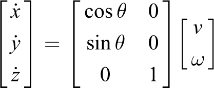
Its kinematic model has the following expression

We can define the state vector

The linear and angular velocities of the robot can be expressed as a function of the linear and angular speeds of the left wheel
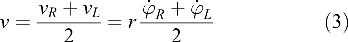

Thus, the kinematic model according to the angular velocities of the left and right drive wheels is written in the following form

Dynamic model
The general dynamic model of a nonholonomic mobile robot can be expressed by equation (6) 19,25

where
Assumption 1
We assume that the mobile robot moves in the horizontal plane and we ignore also the friction forces, thus,
Regarding the previous assumption, the dynamic motion of the robot could be expressed concisely as follows (equation (7))

In view of equation (7), it is clear that for nonholonomic robots, the constraints of motion are introduced using the multiplier constraint

where

The kinetic energy of the right and left wheels


where mc is the mass of the mobile robot without wheels and actuators (DC motors), mw is the mass of each wheel (with actuator), Ic is the moment of inertia of the mobile robot about the vertical axis through the center of mass, Iw is the moment of inertia of each driving wheel with a motor about the wheel axis, and Im is the moment of inertia of each wheel with a motor about the wheel diameter.
With refer to the previous equations, the matrices
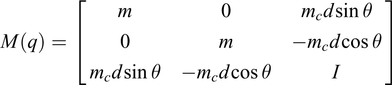


where

It can be easily verified that the transformation matrix S(q) is in the null space of the constraint matrix

Deriving equation (12) with respect to time yields

Substituting equations (12) and (14) into the dynamic motion of the robot expressed by equation (7) leads to

Premultiplying

where
Electrical and mechanical actuator’s model
In applications, where the power involved is less than few kilowatts, the permanent magnet DC motor is widely used. In addition, small engines are very often equipped with a reducing device. It is a question of adapting the motor to the requirements of an application. In fact, the optimum operating speeds of an electric motor, such as a DC motor, are generally higher than the desired speeds. This is particularly true in the case of applications with very low speed and, in particular, for position control. An engine with the speed reducer (ratio N) can be represented by Figure 2.

Simplified diagram of a geared motor with load.
The armature equation is defined by

where
The mechanic equation is

where Cr : resistance torque, Jm : moment of inertia of the MCC, and f: viscous friction of the MCC.
The output torque applied to the wheel after an operation of the speed reducer is given by
Mobile robot control
In this section, we consider the nonholonomic mobile robot schematized by Figure 1 and modeled by kinematic, dynamic, electrical, and mechanical models represented, respectively, by equations (5) and (16) to (18). With such kind of robots, the tracking control issue could be classified in two axes: kinematic or dynamic control. However, it is worth noting that the perplexity in dealing with this category of robots consists on the nonintegrability of nonholonomic constraints. Therefore, the topic of tracking control’s mobile robot is difficult to manage. For that, we propose to design a control architecture that takes into account both models simultaneously. The control architecture is schematized by Figure 3. The kinematic controller represents the high level control of the mobile robot. Its role is to generate the vector of the set speeds used as inputs for the dynamic controller. The objective of the kinematic controller proposed in this article is to elaborate a control law

Block diagram of the proposed control architecture.
For the remainder of this section, we dedicate the first part for a detailed study of the applied kinematic controller accompanied by a proof of stability, while the second part is dedicated to detail the proposed dynamic controller with an interesting proof of stability according to Lyapunov theory.
Kinematic controller
The control law at the kinematic level is based on the stable tracking method, which is frequently used in the literature to cope with the tracking problem. The relationship between the measured variables

where
Thus

We also define the tracking error vector qr
in the reference linked to the robot

where

where k 1, k 2, and k 3 are positive parameters.
Stability proof of the kinematic controller
From (equation (1)), it is clear that the model of the considered robot can be seen as being periodic (with period
Hence, we can say that it is clear that the problem of tracking is periodic with respect to the orientation. This can be observed from the kinematic model using an arbitrary control input and an arbitrary initial condition, resulting in a certain robot trajectory. If the same control input is applied to the robot and the initial condition only differs from the previous one by a multiple of
The periodic nature should also be reflected in the control law used for the tracking. This should mean that one searches for a control law that is periodic with respect to the error in the orientation
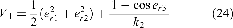
Obviously, the function that is used in this article for the convergence analysis should also be periodic in

where
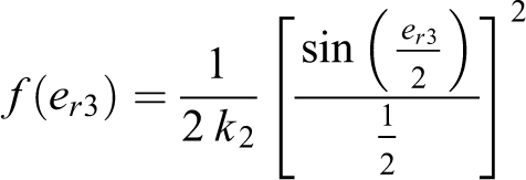
It is obvious that
And now, using the following trigonometric relation:
Hence, the considered positive Lyapunov candidate function is
The development of the derivative of the Lyapunov function V 1 leads to

Taking into account the expressions of the following matrixes

It yields to

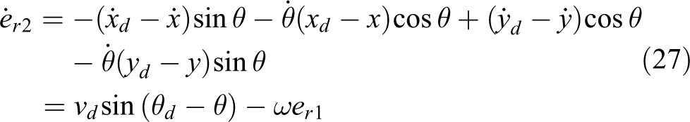

Thus, the tracking error can be expressed as follows

This leads to

Hence, the time derivative
The asymptotic stability of the equilibrium points
Theorem 1
If the control law (22) is applied to the system (29), where k 1, k 2, and k 3 are positive constants. Then, the closed-loop system is asymptotically stable and the tracking errors converge to zero with respect to the following assumptions:
Linear and angular velocities of the reference robot and their first derivatives are assumed to be bounded (i.e, vd
,
The linear and angular velocities of the reference robot do not converge to zero simultaneously.
Proof
Using the proposed control law (22) and the dynamical equations of errors (29), the equations of the closed-loop system are as follows

To prove the stability of the equilibrium points, we will use the following theorem of Barbalat’s lemma. 27
Barbalat’s Lemma
Let
If
Corollary of Barbalat’s Lemma 28
Let
Thus,
Remark
The easiest way to check the uniform continuity of a function
Since V
1 is positive definite Lyapunov function, it is lower bounded by zero. On the other hand, from equation (30), we have
Since the constants k
1, k
2, and k
3 are bounded and considering the assumptions cited in Theorem 1 above,
Until now, only the convergence of

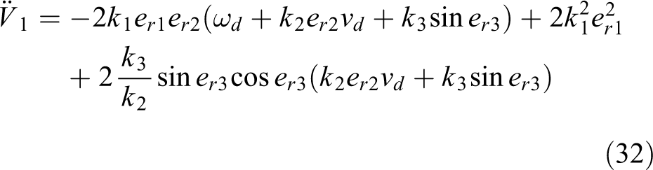
Hence, the second time derivate of
Similar to the previous discussion, it can be easily shown that the second derivative of

since it is proved previously that
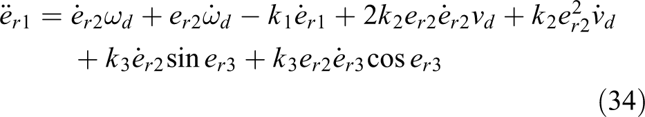
Similarly, consider the dynamical equation of

Similarly, it is easy to show that the second derivative of

According to assumptions of Theorem 1 and equations (35) and (37),
Proposed dynamic control
In this section, we propose a robust adaptive controller as a dynamic controller. The challenge in this part is to take into consideration the external disturbances that appear in the dynamic equation of Lagrange. Indeed, our purpose is to find the adequate controller so that the robot could follow the desired trajectory while resisting against the exogenous disturbances that could deform the path.
With reference to the reduced dynamic equation (16), we have

Finding the suitable control law

To achieve the desired control objective, we found it more interesting to work with the following filtered tracking error (equation (40)), which is defined to facilitate the subsequent design and analysis

The dynamic equation (30) can be described in function of the errors


Assumption 2
Each element of the perturbation vector
Remark 1
The only requirement imposed here is that the perturbation term has to be bounded by an unknown upper bound. The knowledge of this upper bound will be overcome by an adaptive law.
Hence, we propose the following sliding mode-based controller
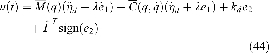
where
The proposed adaptation law is
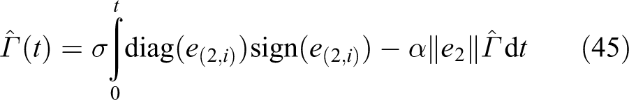
where the speed and resolution of the adaptation of the function
Remark 2
It is worth pointing that the upper bound introduced in this article is represented by a diagonal matrix. This leads to a better estimation of the system uncertainties and ensures a small limited tracking error for each subsystem dynamics.
Stability proof of the proposed dynamic controller
To prove the stability of the proposed robust adaptive controller, the following properties will be used.
Property 1
Property 2
The matrix
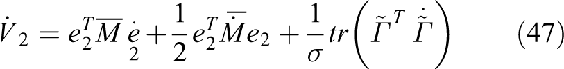
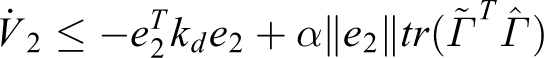
Let us consider the positive Lyapunov-like function (equation (46)) based on quadratic form,
27
which is frequently used for the proof of uniform ultimate bound of the errors’ norms (in this article, the error norms are

where
In the Lyapunov function above, the trace operator is applied since the Lyapunov function should be a scalar. And since (
In this section, we aim to prove that
The derivate of this function is


With reference to Property 2, we have


Using the fact that
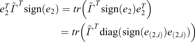
Hence

Using the Cauchy–Schwartz inequality, this yields

This is guaranteed negative since
Consequently,
or

where
Hence,

with


or

Uniform ultimate boundness
At this stage, to show that
Rayleigh–Ritz theorem
Let A be a real symmetric positive definite matrix. Let
Uniform ultimate bound theorem
Let V be a continuous Lyapunov function in time such that

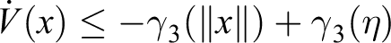
where
We have

We easily deduct that

Furthermore,


Thus, using the Lyapunov theorem extension,
Stability of
To study the stability of the error e 2, we will apply the corollary of Barbalat’s Lemma defined and exploited in the previous section of “Stability proof of the kinematic controller.”
We have V
2 is a definite positive Lyapunov function, therefore, it admits zero as the lower bound. On the other hand, the parameter α is very small and very close to zero, thus, the second term of equation (54) vanishes, which ensures that
Differencing
Thus, using Barbalat Lemma 29

Thus

Therefore, e 2 is globally asymptotically stable. This completes the proof.
Remark 3
The chattering effect from the discontinuity of the sgn() function used in the control law (equation (44)) must be considered in some practical applications. This problem is common in sliding mode control schemes and is usually solved by approximating the discontinuous function sgn() using a continuous function, such as the saturation function. Effects of such approximation on the stability results are analyzed and presented by Benosman and Lum. 30
Comparison with existing robust adaptive laws
To elaborate the advantages of the proposed adaptive law (equation (45)), let us consider two adaptive laws that do not require a priori knowledge of the upper bound of disturbances.
The first adaptive law proposed by Plestan et al. 21,22

where
From this equation, we can notice that when
The second adaptive law proposed by Chen et al. 23 and Koubaa et al. 24

This adaptive law is interesting since it takes into consideration the fact that the system is MIMO. And so, it allows to estimate each upper bound of each subsystem separately. The dynamics of the gain depends directly on the tracking error (sliding variable). It is clear that the value
If we now return to the equation (45) of the adaptive law proposed in this article, it is clear that The knowledge of the upper bound of each disturbance is not necessary. Adaptive estimation is performed for each perturbation of each subsystem bounded by an unknown local upper bound, which provides improved stability and accuracy in the control of finite-time trajectory tracking and robustness against external disturbances. The proposed adaptive law allows its gains to increase to compensate the disturbance effect if As we mentioned previously, the second term of the adaptive law proposed
Simulation results
In this section, simulations are conducted to verify the effectiveness of the proposed control architecture (shown in Figure 3) and its robustness against external disturbances. For that, consider a nonholonomic unicycle mobile robot navigating in 2D space (see Figure 1) and subjected to an external disturbance. We stress that the parameters involved in the sliding mode type controller with an adaptive gain as well as kinematic controller are determined using trial and error method to achieve a satisfactory performance. To put our approach in value, we propose in this section, simulation results, for different scenarios, based on a comparison with the methods,21-–24 already detailed in the previous section. The model of the robot is given by the equations (5) and (16) to (18). The system parameters values are set as follows:
The width of the driving wheels is
The radius of the driving wheels is
The total masse of the robot is
The moment inertia is
The inductance is
The simulation results of two scenarios are shown as follows.
Scenario 1: circular reference trajectory
In this scenario, simulations are conducted for a circular reference trajectory with center
where
Figures 4 to 8 show the results of tracking the circular reference trajectory that results from the use of kinematic controller and dynamic controller proposed by Plestan et al. 21,22 based on the adaptive law of the equation (57).


The dynamic controller parameters are selected by trial and error method as
According to the Figures 4 and 5, this command ensures a good reference trajectory tracking with orientation tracking errors that do not deprive the
Figures 9
to 13 show the results of tracking the circular reference path that results from the use of kinematic controller (equation (22)) and dynamic controller by Chen et al.
23
and Koubaa et al.
24
based on the adaptive law of equation (58). The dynamic controller parameters are selected by trial and error method as


According to Figures 9 and 10, this command ensures a good trajectory tracking with low tracking errors. Orientation tracking errors do not deprive the
Moreover, the torque applied to the right wheel presents some chattering in Figure 12.
Figures 14
to 18 show the results of tracking the circular reference trajectory that results from using the kinematic controller (equation (22)) and our proposed dynamic controller (equations (44) and (45)). The values of the proposed dynamic controller are set

Scenario 1: Desired trajectory versus real trajectory using the proposed adaptive law.

Scenario 1: Position and orientation errors using the proposed adaptive law.

Scenario 1: Proposed adaptive law (equation (45)).

Scenario 1: Torques of right and left wheels using the proposed adaptive law.
Scenario 1: Sliding surface using the proposed adaptive law.
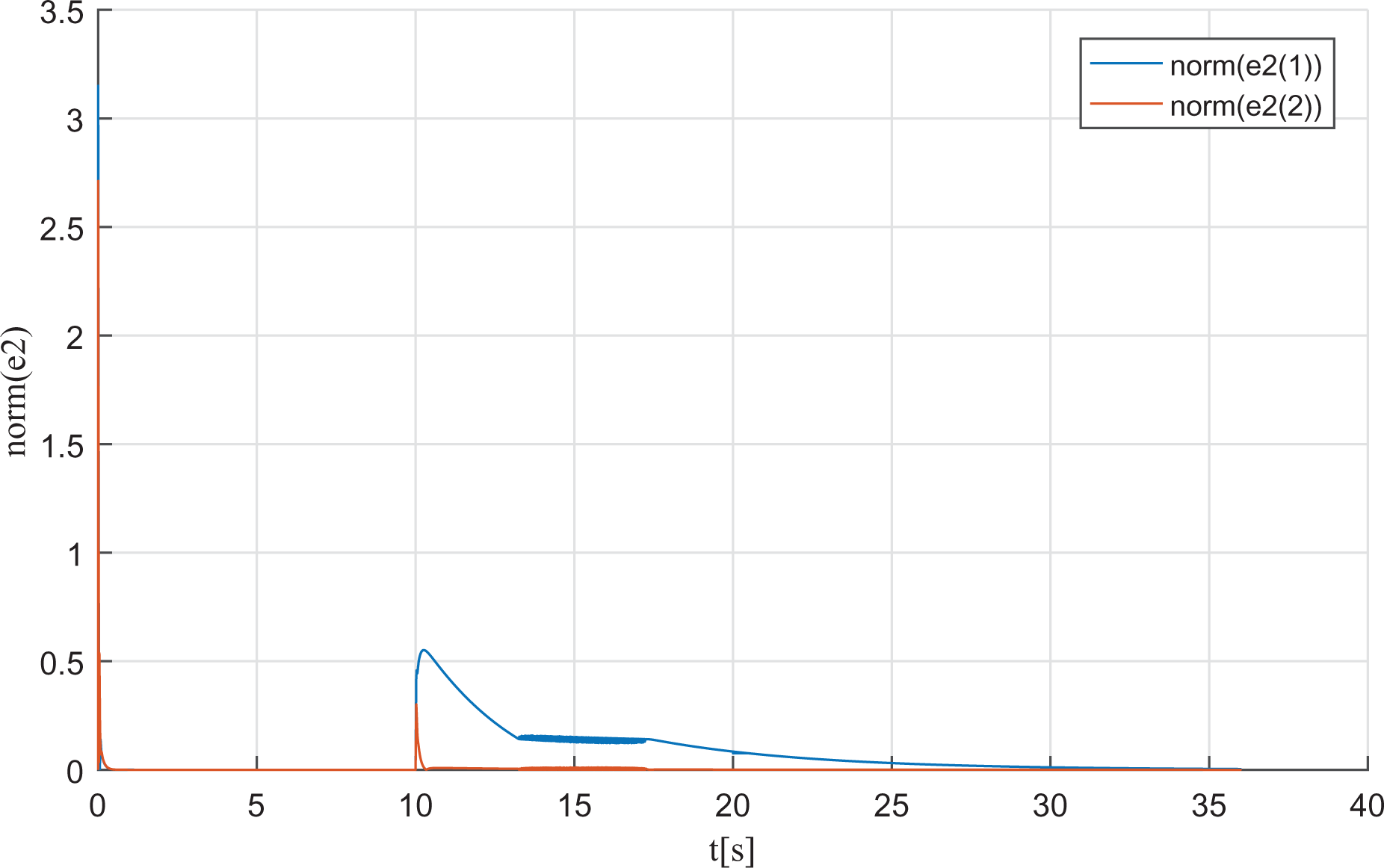
As shown in Figures 14 and 15, the proposed approach ensures a very good tracking trajectory with low tracking errors: orientation tracking errors that do not deprive the
Scenario 2: Lemniscate reference trajectory
Now, we set the desired trajectory as
External disturbances are supposed lasting all the time
In this scenario also, we will compare the results of the trajectory tracking of the proposed dynamic controller with approaches proposed by Plestan et al.21,22 and by Chen et al.
23
and Koubaa et al.
24
The kinematic controller gains applied for the different approaches are
Figures 19
to 22 show the results of tracking the lemniscate reference trajectory that results from the use of kinematic controller (equation (22)) and dynamic controller by Plestan et al.
21,22
based on the adaptive law of equation (57). The dynamic controller parameters are set as

Scenario 2: desired trajectory versus real trajectory using adaptive law (equation (57)) by Plestan et al.


Based on the results in Figures 19 and 20, the tracking trajectory is acceptable with position errors less than

Figures 24
to 28 show the results of tracking the lemniscates reference path that results from the use of kinematic controller (equation (22)) and dynamic controller by Chen et al.
23
and Koubaa et al.
24
based on the adaptive law of equation (58). The dynamic controller parameters are


From the results given in Figures 24 and 25, the tracking trajectory is acceptable with position errors less than
Figures 29
to 33 show the results of tracking the lemniscate reference trajectory that results using the kinematic controller (equation (22)) and our proposed dynamic controller (equations (44) and (45)). The values of the proposed dynamic controller are set:

Scenario 2: desired trajectory versus real trajectory using the proposed adaptive law.

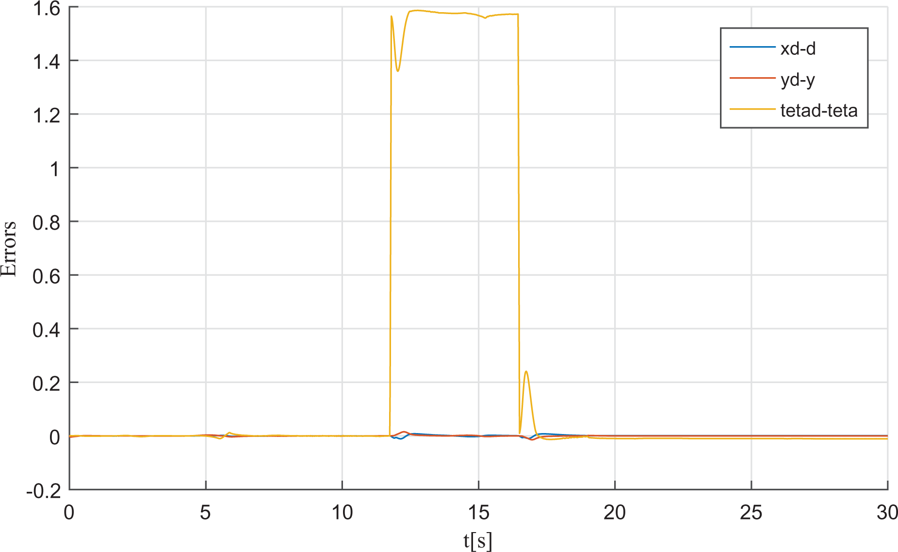
Scenario 2: Position and orientation errors using the proposed adaptive law.

Scenario 2: Proposed adaptive law.

Scenario 2: Torques of right and left wheels using the proposed adaptive law.

Scenario 2: Sliding surface using the proposed adaptive law.
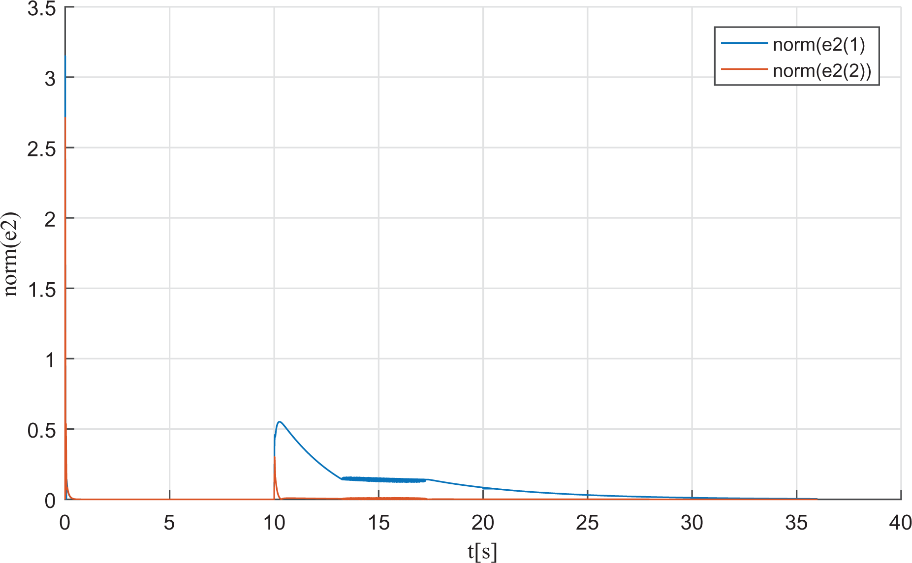
The results shown in Figures 29 and 30 show clearly that the controllers proposed have the ability to stabilize the global nonholonomic mobile robot system and provide a good tracking performance with position errors less than
The results prove the effectiveness of the proposed controller, with robust and adaptive terms, where each upper bound local is only sensitive to its local disturbance. It is clear that the estimated parameters remain stable and that each upper bound converges toward a specific value (Figure 31) while the sliding surface converges to 0 (Figure 33), guaranteeing a small tracking error despite the local external disturbance.
Moreover, the torques’ oscillations (Figure 33) are negligible comparing to the results obtained in Figures 27 and 24.
Discussion
To conclude, after the follow-up results of the trajectories tracking illustrated in scenarios 1 and 2, we can extract the following remarks. The dynamic controller proposed in this article is more efficient than the other controllers since it ensures: Good robustness against external disturbances; Stability of the nonholonomic robotic system studied; Good accuracy of trajectory tracking; Speed of convergence of the sliding surface toward 0 without chattering; Minimum of trajectory tracking errors; Minimum of chattering in the produced torques; Values of estimated gains bounded and therefore no problems of over / underestimation of parameters.
Conclusion
In this article, we have studied and solved the problem of trajectory tracking of nonholonomic mobile robot subjected to external disturbances. To study the subject from all sides, we have firstly detailed the kinematic and dynamic models of nonholonomic robot as well as the electric and dynamic models of the actuators. Then, we proposed a kinematic controller to elaborate a control law, which makes it possible to cancel the posture of error. A sliding mode-based adaptive gain controller is then designed, stabilizing each of the subsystems, to compensate the negative influence of the external disturbances. The interesting idea in this article is that we have proposed an adaptive integral law for the estimation of the unknown upper bound of each subsystem separately using the diagonal matrix. Based on Lyapunov theory, stability of the two proposed controllers was proved. The performance of the control architecture based on kinematic and dynamic controllers is illustrated on two simulation examples based on a comparative study with two other dynamic controllers-based sliding mode with adaptive law. The results of simulations have shown that the proposed approach is more efficient since it allows having lower tracking errors, good robustness and accuracy, and also, it overcomes the problems of under/over estimation. In addition, chattering is negligible compared to other methods.
Footnotes
Declaration of conflicting interests
The author(s) declared no potential conflicts of interest with respect to the research, authorship, and/or publication of this article.
Funding
The author(s) received no financial support for the research, authorship, and/or publication of this article.