Sage Journals: Discover world-class research

Abstract

With the growth of the number of elderly and disabled with motor dysfunction, the demand for assisted exercise is increasing. Wearable power assistance robots are developed to provide athletic ability of limbs for the elderly or the disabled who have weakened limbs to better self-care ability. Existing wearable power-assisted robots generally use surface electromyography (sEMG) to obtain effective human motion intentions. Due to the characteristics of sEMG signals, it is limited in many applications. To solve the above problems, we design a long short-term memory (LSTM) neural network model based on human mechanomyography (MMG) signals to estimate the motion acceleration of knee joint. The acceleration can be further calculated by the torque required for movement control of the wearable power assistance robots for the lower limb. We detect MMG signals on the clothed thigh, extract features of the MMG signals, and then, use principal component analysis to reduce the features’ dimensions. Finally, the dimension-reduced features are inputted into the LSTM neural network model in time series for estimating the acceleration. The experimental results show that the average correlation coefficient (R) is 94.48 ± 1.91% for the estimation of acceleration in the process of continuously performing under approximately π/4 rad/s. This approach can be applied in the practical applications of wearable field.

Keywords

Knee joint MMG PCA LSTM acceleration estimation

Introduction

With the aggravation of the population aging process, the number of elderly people is growing rapidly. The world’s population aged over 60 will grow from 12% in 2015 to 22% by 2050.¹ On the other hand, the number of amputees has increased due to vascular diseases, traffic accidents, work-related injuries, and accidental injuries. According to the Sixth National Census, the total number of people with disabilities was approximately 85.02 million in China by the end of 2010, of which 24.72 million were physically disabled, ranking first among all types of disabilities.² Therefore, it is urgent to solve the problems of inconvenience of life and travel caused by the weakening of the limbs of the above people, which is a major social problem that needs to be solved at present.

Many scholars and institutions have used wearable robot technology to research wearable power assistance robots in the elderly or the disabled fields. Wearable power assistance robots are developed to provide athletic ability of limbs for the elderly or the disabled who have weakened limbs to better self-care ability.³ It is great significance and application prospects to meet the growing current situation of elderly and physically disabled people.

With the development of signal detection, signal processing, and data fusion technology, wearable power assistance robots have gradually evolved from a passive way of accepting human instructions to a way of actively recognizing and understanding human motion intentions. Early active and passive wearable power assistance robot products mainly use angle, force, acceleration, and other physical information as control sources. Since the external kinematic parameters can only passively reflect people’s motion intentions, the actual information obtained lags behind human motion.⁴ Biological signals can intuitively reflect the intention and state of human motion and precede the occurrence of macromotion. If the physiological signals of the human body can be used as control sources, the control of the wearable power assistance robot and the human body will be more coordinated and smoother. The research of modern human anatomy has shown that the surface electromyography (sEMG) signal is closely related to muscle activity. The sEMG signal can be generated about 30–100 ms before muscle activity. The sEMG signal can be used to estimate and evaluate muscle function, muscle strength, and fatigue state.⁵ Through collecting and processing the sEMG signals of the skin surface, the features of the signals can be extracted as the source of control signals for the wearable power assistance robot control system.⁶ However, most of the sEMG sampling electrodes require to be attached on the skin, which restricts its application.⁷

The research has shown that not only sEMG signals are produced but also a low-frequency mechanical vibration signal is produced following the muscle activity.^8,9 Researchers use mechanomyography (MMG) to describe the mechanical vibration signal. MMG signal can provide information about the number of muscle motor units and the excitation rate.¹⁰ The MMG signal reflects the characteristics of muscle activity during motion. Through effective features extraction and classification of MMG signal, the intention of human motion can be predicted in advance. Researchers have tried to control the wearable power assistance robots based on the MMG signals.¹¹ MMG is a vibration signal generated by muscle contraction during motion.¹² The MMG signal acquisition does not need to be very accurate with the placement of sensors.¹³ At the same time, using the MMG signals has such advantages as the low cost of acquisition system, anti-interference, and robustness. In addition, the data can be effectively collected by tying the sensor to the relevant parts through clothes without directly contacting with the skin so that data collecting is not affected by the change in resistance caused by sweat or the temperature of the skin surface.¹⁴ MMG signals are more applicable to applications in sports, wearables, and so on.

Alves and Chau¹⁵ made use of two acceleration sensors to detect the MMG signals of forearm muscle activity, and the recognition rate of the classifier reached 89 ± 2% for three types of hand motion. Silva et al.¹⁶ constructed classifiers based on the MMG signals for controlling the closing and opening of a prosthesis. The accuracy reached approximately 70%. Zeng¹⁷ used only a single acceleration sensor to detect the MMG signals of forearm muscle activity. Through principal component analysis (PCA) and the construction of a quadratic classifier, the recognition rate of hand motion reached approximately 80% in real-time prosthetic hand control experiments. Ibitoye et al.¹⁸ built a support vector regression model based on MMG signals to estimate the knee torque induced by neuromuscular electrical stimulation. When using the Gaussian support vector kernel, the decision coefficient between the actual torque and the estimated torque reached 94%. Dzulkifli et al.¹⁹ constructed a neural network model based on the quadricep MMG signals to predict the knee torque to solve the situation that the muscle torque could not be quantified independently. It was found that the average accuracy of the predicted knee joint elongation torque reached 79 ± 14%, which provided a safer automatic control for the standing of patients with a complete spinal cord injury. Youn and Kim²⁰ used acceleration sensors (ADXL202JE) to record the MMG signals of the brachioradialis and biceps muscles. Meanwhile, they extracted features of the MMG signals as inputs to the neural network model. Then, the bend force of the elbow joint was estimated by the neural network algorithm.

In this study, we take the knee joint as the research object and design a long short-term memory (LSTM) neural network²¹ that uses MMG signals for estimating the motion acceleration of knee joint. The acceleration can be further calculated by the torque required for movement control of the wearable power assistance robots for the lower limb. We detect the MMG signals on the clothed thigh. Some time- and frequency-domain features of the MMG signals are extracted, and then, PCA²² is used to reduce the features’ dimensions. Finally, the dimension-reduced features are inputted into the LSTM neural network model in time series for estimating the acceleration of knee joint.

The rest of the article is organized as follows. In the second section, we introduce the LSTM neural network. In the third section, the experiment and signal preprocessing are described, including the experimental procedure, the MMG signal preprocessing, the feature extraction, the features dimension reduction, and the implementation of the LSTM neural network model. The experimental results and discussion are presented in the fourth section. Finally, the conclusion is shown in the fifth section.

Long short-term memory neural network

Recurrent neural network (RNN) is a neural network for processing sequence data.²³ RNN remembers the previous information. The previous information is applied to the calculation of the current output. Figure 1 shows the structure of the RNN. The neurons of the hidden layer are connected. The input of the current time hidden layer includes not only the input of the current time but also the output of the previous moment hidden layer. Figure 2 shows the unfolding of a neuron of the hidden layer on the input sequence. The output value O of a certain neuron of the hidden layer at the current moment not only depends on the input x of the neuron at the current moment but also depends on the output value O _t−1 and the memory value S _t−1 of the hidden layer at the previous moment.

Figure 1.

The structure of the RNN. RNN: recurrent neural network.

Figure 2.

The unfolding of a neuron of the hidden layer.

The LSTM neural network is a deformed structure of RNN. The LSTM neural network combines long-time and short-time series-related information through subtle gate control to better preserve the long-time series-related information and to control the gradient flow, which solves the problem of gradient disappearance to a certain extent. The unit composition of the LSTM block is shown in Figure 3. Each LSTM block is equal to a neuron in the hidden layer of RNN. The LSTM neural network uses a gate structure to remove or increase the memory information of a block, to retain the important information, and to remove the unimportant information. The LSTM block consists of the forget gate, input gate, and output gate. These units are connected in series to learn and store long-term and short-term series-related information.

Figure 3.

Unit composition of the LSTM block. LSTM: long short-term memory.

The first unit is the forget gate, which decides how much information of unit memory S _t−1 from the previous block is retained ${\tilde{S}}_{t - 1}$ in the current block. The forget gate includes a sigmoid function and a pointwise multiplication operation. The sigmoid function is as follows

f_{t} = σ (W_{f} (O_{t - 1}, x_{t}) + b_{f})

where W_f is the weight parameter, O_t ₋₁ is the output of the previous hidden layer, x_t is the input for the current block, and b_f is a bias term.²⁴

${\tilde{S}}_{t - 1}$ is expressed as follows:

{\tilde{S}}_{t - 1} = f_{t} * S_{t - 1}

where f_t is the result from formula (1), S_t ₋₁ is the unit memory from the previous block, and ${\tilde{S}}_{t - 1}$ is the memory preservation from the previous block to the current block.²⁵

The second unit is the input gate, which decides how much information of the input x_t is saved to the unit memory S_t at the current moment.²⁶ The input gate includes a sigmoid function, a tan h function, and a pointwise multiplication operation. The sigmoid function is as follows

i_{t} = σ (W_{i} (O_{t - 1}, x_{t}) + b_{i})

where i_t is the decision vector of the unit memory at the current moment, W_i is the weight parameter, and b_i is a bias term.

The tan h function is as follows

{\tilde{S}}_{t} = tan h (W_{c} (O_{t - 1}, x_{t}) + b_{c})

where S˜_t is the candidate information of the unit memory at the current moment, W_c is the weight parameter, and b_c is a bias term.²⁶

The pointwise multiplication operation is as follows

S_{t} = i_{t} * {\tilde{S}}_{t} + {\tilde{S}}_{t - 1}

where S_t is the output of unit memory at the current block.

The third unit is the output gate, which decides how much information of the unit memory S_t is outputted to the output O_t at the current block.²⁶ The output gate includes a sigmoid function, a tan h function, and a pointwise multiplication operation. The sigmoid function is as follows

h_{t} = σ (W_{h} (O_{t - 1}, x_{t}) + b_{h})

where h_t is the part of the unit memory output at the current block, W_h is the weight parameter, and b_h is a bias term.

The tan h function and the pointwise multiplication operation are as follows

O_{t} = tan h (S_{t}) * h_{t}

where O_t is the output at the current block.

Finally, the output O_t and the output of the unit memory S_t at the current block are inputted into the next moment hidden layer. The process is repeated. The difference between the output of LSTM neural network and the real training samples is minimized by learning and optimizing the weight parameters and bias terms of the model.

Experiment and signal preprocessing

Experimental procedure

The right knee joint acceleration is estimated while the right knee joint is performing isokinetic knee extension and flexion motions in this experiment. Meanwhile, the Medical Ethics Committee of Hefei Institutes of Physical Sciences authorized the experiment. We select four healthy young people as experimental participants, who aged between 24 and 30 years. We refer to the knee joint swing angle (approximately 60°) during normal walking. In the sitting position, participants are required to continuous extension and flexion of the knee joint under approximately π/4 rad/s (SV) and π/2 rad/s (FV) for 30 s, as shown in Figure 4. Each participant has a complete rest between two different speed experiments.

Figure 4.

Knee joint continuous motion.

According to the anatomy of human motion, we select the superficial muscles that control the continuous motion of the knee joint for MMG signal detection. We select semitendinosus, biceps femoris, vastus medialis, vastus lateralis, and rectus femoris from the thigh, as shown in Figure 5.

Figure 5.

Muscle diagram—1: semitendinosus; 2: biceps femoris; 3: vastus medialis; 4: vastus lateralis; and 5: rectus femoris.

Figure 6 shows the collection and store system of data. According to the previous experiment, the MMG sensor is made by a triaxial accelerometer (model ADXL335).²⁷ The positive direction of the z-axis is placed perpendicular to the skin outward. The output of z-axis measures the MMG signal. Five MMG sensor positions are selected to be in the corresponding muscle’s central region and are bound to the clothes by kneepad-like straps. The acceleration sensor is made by a dual-axis accelerometer evaluation board (model ADXL203EB), which measures the real linear acceleration of the knee joint to calculate the angular acceleration and the torque.²⁸ The acceleration sensor is placed on the clothes against the medial ankle joint of the shin (the X-axis is perpendicular to the shin and points forward in front of the body), and it is bound to the leg by kneepad-like straps for following the rotation of the knee joint. The acceleration is calculated according to change in the acceleration sensor data of the motion of knee extension and flexion, which marks the acceleration category label. A collector (model NI USB-6215) collects signals of the MMG sensors and acceleration sensor. The collection frequency of the data is 2000 Hz. The collector is connected to the host computer through the USB interface. Meanwhile, the data are shown and saved by the program of the host computer.

Figure 6.

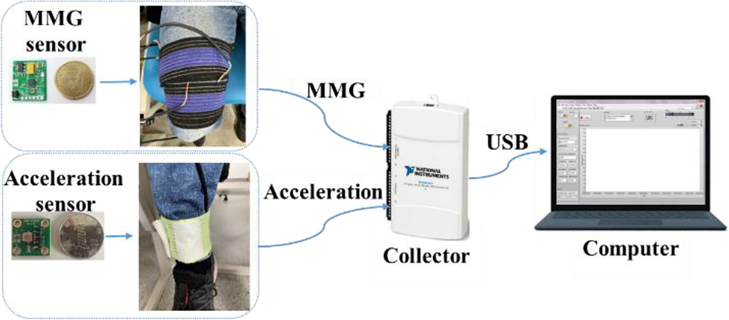
Collection and store system of data.

Signal preprocessing

We use sliding window and stepping methods to continuously read signal flow. With reference to the previous related research,¹⁴ we chose a 250 ms (500 samples) sliding window and 62.5 ms (150 samples) increment. For the MMG signals, we use a 5–100 Hz third-order Butterworth band-pass filter to filter out the human motion trajectory and environmental noise. Figure 7 shows the filter effect on the MMG data of the rectus femoris. For the acceleration signal, we use a 1.5-Hz fourth-order Butterworth low-pass filter to filter out high-frequency noise. Figure 8 shows the filter effect on the acceleration data.

Figure 7.

Filter effect on the MMG data. MMG: mechanomyography.

Figure 8.

Filter effect on the acceleration data.

Feature extraction and dimensions reduction

In this experiment, we extract features from the set sliding window of each MMG signal. Root mean square, mean absolute value, zero-crossing rate, slope sign change, and waveform length of the MMG signals are selected as the time-domain features.²⁹ Median frequency,³⁰ mean power frequency,³⁰ and mean frequency²⁹ of the MMG signals are selected as the frequency-domain features. Sample entropy and Spearman’s correlation coefficients of the MMG signals are selected as other features.³¹

To improve the speed of data processing, the 48-dimensional time and frequency domain feature data constructed from five MMG sensors data are reduced dimensionally by the PCA. To implement the PCA, we call the PCA function in MATLAB 2018A. Principal components of the training samples whose cumulative contribution rate is more than 90% are obtained as new input features of the training model. The new features contain 18 principal components. Figure 9 shows the contribution rate of the principal components. Meanwhile, the corresponding transformation matrix of training samples is obtained. The test samples are multiplied by the transformation matrix to obtain the new features of the test samples. The new feature data of the training samples are normalized using the Z-score method³² and then are inputted into the LSTM neural network model. The new feature data of the test samples are normalized using the mean and standard deviation of the training samples.

Figure 9.

The contribution rate of the components.

Implementation of the long short-term memory neural network model

The implementation process of the LSTM neural network model is shown in Figure 10. The five-channel original MMG and acceleration signals are filtered by Butterworth filter. The feature extraction of the MMG signals is performed by the sliding window method. The feature data are reduced dimensionally by the PCA and then normalized using the Z-score method. In addition, the corresponding category labels are generated by the mean value of the acceleration data in each sliding window. Each participant can yield nearly 390 sets of valid time-series data (acceleration-MMG). According to the time series, we select the first 80% of valid data as the training samples. Then, we select the last 20% of valid data as the test samples.

Figure 10.

Implementation process of the LSTM neural network model. LSTM: long short-term memory.

To implement the LSTM neural network, we call deep learning toolbox in MATLAB 2018A. The designed LSTM neural network is shown in Figure 11. The LSTM neural network that we design contains four layers. First, the time-series features are inputted into the input layer according to the time sequence. Second, the input layer is connected to the LSTM layer. Third, the LSTM layer is connected to the fully connected layer. Fourth, the fully connected layer is connected to the regression layer. Finally, the regression layer outputs the estimated acceleration. The input layer contains 18-dimensional feature data according to the result of the PCA algorithm. The LSTM layer contains 400 neurons. During model training, we set the number of iterations is 400, and the initial learning rate is 0.005. After 200 iterations, the learning rate decreases according to a fading factor of 0.2. Meanwhile, to compare the superiority of the LSTM neural network model, we set up 50 and 100 neurons in the fully connected layer to carry out comparative experiments.

Figure 11.

The structure of the LSTM neural network. LSTM: long short-term memory.

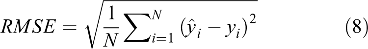
According to the time series, we input the training samples of each participant into the LSTM neural network to train the neural network model. According to the time series, we input the test samples of each participant into the trained model, respectively. We, respectively, calculate the correlation coefficient (R) and root mean square error (RMSE) of the test samples to assess the accuracy. Finally, the neural network model with the highest R is selected. The calculation formulas of R and RMSE are as follows

R M S E = \sqrt{\frac{1}{N} \sum_{i = 1}^{N} {({\hat{y}}_{i} - y_{i})}^{2}}

R = Cov ({\hat{y}}_{i}, y_{i}) / \sqrt{D ({\hat{y}}_{i}) \sqrt{D (y_{i})}}

where ${\hat{y}}_{i}$ is the estimated value of the i’th test sample; y_i is the observed value of the i’th test sample; $D ({\hat{y}}_{i})$ is the variance of the estimated value of the test samples; D(y_i ) is the variance of the observed value of the test samples; and $Cov ({\hat{y}}_{i}, y_{i})$ is the covariance between the estimated value and the observed value of the test samples.

Experimental results and discussion

Tables 1 and 2 present R values on the test samples under SV and FV for four participants, when the fully connected layer contains 50 and 100 neurons, respectively. The mean of R is 88.43% under SV and FV for four participants, when the fully connected layer contains 50 neurons. The experimental results with 50 neurons are better than the experimental results with 100 neurons in the fully connected layer. The LSTM neural network model with 50 neurons in the fully connected layer has better generalization ability. Finally, we select the LSTM neural network model with 50 neurons in the fully connected layer. The following discussion is the experimental results based on containing 50 neurons in the fully connected layer.

Table 1.

Comparison of the R values of the different neural network model on the test samples under SV for four participants.

	P1	P2	P3	P4
100 Neurons	96.06%	91.53%	95.74%	93.17%
50 Neurons	96.64%	93.05%	95.54%	92.71%

P: participant.

Table 2.

Comparison of the R values of the different neural network model on the test samples under FV for four participants.

	P1	P2	P3	P4
100 Neurons	85.06%	75.69%	76.59%	90.50%
50 Neurons	85.48%	76.15%	76.87%	90.97%

P: participant.

Figure 12 (a) to (e) shows the waveform cross-section of the filtered MMG signals from the test samples under SV. The 77 sets of MMG signal values are obtained by the sliding window and stepping methods from approximately 11,700 MMG signal values. We observe that the waveform of MMG signals change similarly with knee flexion and extension motion. The selected MMG signals can effectively reflect the motion information of knee joint. Figure 8(f) shows the estimated value and the observed value of the acceleration from the test samples under SV. The high correlation between the filtered observations of acceleration and the estimated values of acceleration shows that the model we designed performs well. The model that used the MMG signals can effectively control the motion acceleration of knee joint.

Figure 12.

(a–e) Waveform sections of the filtered MMG signals from a participant under SV and the estimated value of the acceleration.

Figures 13 and 14 show the R and RMSE of the LSTM neural network model on the test sample under SV and FV for four participants. For the average of four participants, R is 94.48 ± 1.91%, and RMSE is 0.0849 ± 0.0130 under SV, while R is 82.37 ± 7.13%, and RMSE is 0.0503 ± 0.0166 under FV. We observe that a better R can be obtained under SV. The standard deviation of R is also relatively small under SV. RMSE is similar under SV and FV. The LSTM neural network model can better estimate the motion acceleration of knee joint under SV. The results show that the LSTM neural network model has high fitting ability under SV. The results show that it is feasible to estimate knee joint acceleration using the MMG signals based on the LSTM neural network model.

Figure 13.

Comparison of the R values of the neural network model on the test samples under SV and FV for four participants.

Figure 14.

Comparison of the RMSE values of the neural network model on the test samples under SV and FV for four participants. RMSE: root mean square error.

Conclusions

In this study, we design an LSTM neural network model based on the MMG signals to estimate the motion acceleration of knee joint. Performance of the model is compared under SV and FV for four participants. The experimental results show that the model can better estimate the motion acceleration of knee joint under SV. The whole results show that the LSTM neural network model performs well. This approach promotes the application of the angular acceleration and the torque required for movement control of the wearable power assistance robots for the lower limb. Meanwhile, it improves the flexibility, comfort, and wearable ability of the wearable power assistance robots for the lower limb.

Footnotes

Declaration of conflicting interests

The author(s) declared no potential conflicts of interest with respect to the research, authorship, and/or publication of this article.

Funding

The author(s) disclosed receipt of the following financial support for the research, authorship, and/or publication of this article: This work was supported in part by the Strategic Priority Research Program of the Chinese Academy of Sciences under Grant No. XDA22040303, Natural Science Research Project of Anhui Jianzhu University No. JZ192012 and the State Key Laboratory of Transducer Technology.

ORCID iD

Chenlei Xie

References

Yang

Isaia

Brown

LJE

, et al. E-textiles for healthy ageing. Sensors 2019; 19: 4463.

Zhao

. China Disabled Persons’ Federation released the latest data of disabled population in China. Disability Research 2012; 1: 11–11.

. The research of motion pattern recognition and joint moment analysis of human lower limb based on sEMG. MS Thesis, Department of SOMAEE, Soochow University, Shanghai, China, 2016.

Zhang

Lan

Fan

. Technical development and trend analysis of smart knee prostheses. Chinese J Rehabilitation Med 2017; 32: 451–453.

Staudenmann

Roeleveld

Stegeman

, et al. Methodological aspects of SEMG recordings for force estimation–a tutorial and review. J Electromyogr Kinesiol 2010; 20: 375–387.

Bai

Yao

Yang

, et al. Upper arm force sEMG analysis based on SVM. In: 2018 IEEE International Conference on Intelligence and Safety for Robotics (ISR), Shenyang, China, 24–27 August 2018, pp. 569–574. Washington, DC: IEEE.

Takei

Yoshida

Kobayashi

. Wearable muscle training and monitoring device. In: 2018 IEEE Micro Electro Mechanical Systems (MEMS), Belfast, United Kingdom, 21–25 January 2018, pp. 55–58. Washington, DC: IEEE.

Orizio

Muscle sound: bases for the introduction of a mechanomyographic signal in muscle studies. Crit Rev Biomed Eng 1993; 21(3): 201–243.

Beck

Housh

Johnson

, et al. Mechanomyographic amplitude and mean power frequency versus torque relationships during isokinetic and isometric muscle actions of the biceps brachii. J Electromyogr Kinesiol 2004; 14(5):555–564.

10.

Evetovich

Housh

Stout

, et al. Mechanomyographic responses to concentric isokinetic muscle contractions. Eur J Appl Physiol 1997; 75(2): 166–169.

11.

Park

Kim

, et al. Custom optoelectronic force sensor based ground reaction force (GRF) measurement system for providing absolute force. In: 2016 13th international conference on ubiquitous robots and ambient intelligence (URAI), Xian, China, 19–22 August 2016, pp. 75–77. Washington, DC: IEEE.

12.

Talib

Sundaraj

Lam

. Choice of mechanomyography sensors for diverse types of muscle activities. J Telecommun Electron Comput Eng 2018; 10: 79–82.

13.

Plewa

Samadani

Orlandi

, et al. A novel approach to automatically quantify the level of coincident activity between EMG and MMG signals. J Electromyogr Kinesiol 2018; 41: 34–40.

14.

Wang

Huang

, et al. Real-time continuous recognition of knee motion using multi-channel mechanomyography signals detected on clothes. J Electromyogr Kinesiol 2018; 38: 94–102. Washington, DC: IEEE.

15.

Alves

Chau

. Recognition of forearm muscle activity by continuous classification of multi-site mechanomyogram signals. In: 2010 annual international conference of the IEEE engineering in medicine and biology, Buenos Aires, Argentina, 31 August–4 September 2010, pp. 3531–3534.

16.

Silva

Heim

Chau

. MMG-based classification of muscle activity for prosthesis control. In: 26th annual international conference of the IEEE engineering in medicine and biology society, San Francisco, USA, 1–5 September 2004, pp. 968–971. Washington, DC: IEEE.

17.

Zeng

Mechanomyographic hand-motion pattern identification and its application in prosthetic hand manipulation. MS Thesis, Department of SOMAPE, East China University of Science and Technology, Shanghai, China, 2010.

18.

Ibitoye

Hamzaid

Wahab

AKA

, et al. SVR modelling of mechanomyographic signals predicts neuromuscular stimulation-evoked knee torque in paralyzed quadriceps muscles undergoing knee extension exercise. Comput Biol Med 2020; 117: 103614.

19.

Dzulkifli

Hamzaid

Davis

, et al. Neural network-based muscle torque estimation using mechanomyography during electrically-evoked knee extension and standing in spinal cord injury. Front Neurorobot 2018; 12: 50.

20.

Youn

Kim

. Feasibility of using an artificial neural network model to estimate the elbow flexion force from mechanomyography. J Neurosci Methods 2011; 194: 386–393.

21.

Bouktif

Fiaz

Ouni

, et al. Optimal deep learning LSTM model for electric load forecasting using feature selection and genetic algorithm: comparison with machine learning approaches. Energies 2018; 11: 1–20.

22.

Jolliffe

Cadima

. Principal component analysis: a review and recent developments. Philos Trans Royal Soc A: Math Phys Eng Sci 2016; 374: 1–16.

23.

Zhou

Huang

, et al. Large scale recurrent neural network on GPU. In: 2014 international joint conference on neural networks (IJCNN), Beijing, China, 6–11 July 2014, pp. 4062–4069. Berlin, BER: Springer-Verlag.

24.

Huan

, et al. Prediction of dissolved oxygen in aquaculture based on gradient boosting decision tree and long short-term memory network: a study of Chang Zhou fishery demonstration base, China. Comput Electron Agric 2020; 175: 105530.

25.

Zhu

Yang

Guo

, et al. Short-term load forecasting for electric vehicle charging stations based on deep learning approaches. Appl Sci 2019; 9: 1723.

26.

Liu

. Research on short-term traffic flow prediction model based on RNN-LSTM. In: International conference on AI and big data application (AIBDA 2019), Guangzhou, China, 20–22 December 2019, pp. 12–17.

27.

Huang

Wang

, et al. A CNN-SVM combined model for pattern recognition of knee motion using mechanomyography signals. J Electromyogr Kinesiol 2018; 42: 136–142.

28.

Knudson

. Fundamentals of biomechanics. Berlin: Springer Science & Business Media, 2007.

29.

Fan

Wang

, et al. A canonical correlation analysis based EMG classification algorithm for eliminating electrode shift effect. In: 2016 38th annual international conference of the IEEE engineering in medicine and biology society (EMBC), Florida, USA, 16–20 August 2016, pp. 867–870. Washington, DC: IEEE.

30.

Abdelouahad

Belkhou

Jbari

, et al. Time and frequency parameters of sEMG signal—force relationship. In: 2018 4th international conference on optimization and applications (ICOA), Mohammedia, Morocco, 26–27 April 2018, pp. 1–5. Washington, DC: IEEE.

31.

Xie

Wang

, et al. Angular velocity estimation of knee joint based on MMG signals. In: International conference on intelligent robotics and applications, Shenyang, China, 8–11 August 2019, pp. 15–25. Berlin, BER: Springer-Verlag.

32.

Saranya

Manikandan

. A study on normalization techniques for privacy preserving data mining. Int J Eng Technol 2013; 5: 2701–2704.

A long short-term memory neural network model for knee joint acceleration estimation using mechanomyography signals

Abstract

Keywords

Introduction

Long short-term memory neural network

Experiment and signal preprocessing

Experimental procedure

Signal preprocessing

Feature extraction and dimensions reduction

Implementation of the long short-term memory neural network model

Experimental results and discussion

Conclusions

Footnotes

Declaration of conflicting interests

Funding

ORCID iD

References