Sage Journals: Discover world-class research

Abstract

Inspired by the phototropism of plants, a novel variant of the rapidly exploring random tree algorithm as called phototropism rapidly exploring random tree is proposed. The phototropism rapidly exploring random tree algorithm expands less tree nodes during the exploration period and has shorter path length than the original rapidly exploring random tree algorithm. In the algorithm, a virtual light source is set up at the goal point, and a light beam propagation method is adopted on the map to generate a map of light intensity distribution. The phototropism rapidly exploring random tree expands its node toward the space where the light intensity is higher, while the original rapidly exploring random tree expands its node based on the uniform sampling strategy. The performance of the phototropism rapidly exploring random tree is tested in three scenarios which include the simulation environment and the real-world environment. The experimental results show that the proposed phototropism rapidly exploring random tree algorithm has a higher sampling efficiency than the original rapidly exploring random tree, and the path length is close to the optimal solution of the rapidly exploring random tree* algorithm without considering the non-holonomic constraint.

Keywords

Rapidly exploring random tree phototropism virtual light P-RRT RRT*

Introduction

Path planning is a fundamental research topic in the field of robotics. The purpose of path planning is to find a collision-free path for the mobile robot from the current configuration to the desired configuration with the least possible cost, including shortest path length, minimum moving time, minimum energy consumption, and so on. In the past decades, numerous approaches for path planning have been proposed, including graph-based methods,^1
–3 artificial potential field (APF) method,⁴ reinforcement learning (RL),^5,6 sample-based methods,^7
–9 and so on.

The common graph-based methods include A*, Dijkstra, D*, and so on. These methods can find a high-quality path depend on the resolution of the discrete map. The higher the map resolution is, the stronger the ability of searching path is, but the efficiency of searching will be reduced and the resulting path is not smooth enough to be tracked by the robot.

The APF was first proposed by Khatib.¹⁰ The principle of APF method is to construct an APF in the working environment of mobile robots. The goal point will generate attractive potential field and the obstacle will generate repulsive potential field. This method is simple in calculation and has good real-time performance. However, there are significant problems that inherent to APF method, such as trap solution due to local minima, oscillations in narrow passages, and so on.

RL is a machine learning framework for sequential decision-making problems.¹¹ In the RL framework, the robot can learn an optimal behavior policy through trial-and-error by interacting with the working environment. Zuo et al.¹¹ propose an improved A* algorithm which uses the least squares policy iteration to learn a near-optimal local planning policy that can generate smooth trajectories under kinematic constraints of the robot. Plaza et al.¹² combine the RL strategies with cell-mapping techniques to solve the optimal-control problem for the car-like robot.

Prior sample-based methods, like probabilistic roadmaps and rapidly exploring random tree (RRT),¹³ work well in the field of path planning due to their efficiency and simplicity. Owing to its great performance, RRT has been one of the most popular sample-based path planning algorithms, which can be used in high dimensional spaces under the non-holonomic constraint such as car-like robot. In recent years, many variants of RRT algorithm have been proposed. Some variants aim to improve the sampling efficiency of the explore tree, but the optimization performance is poor.^14,15 Some other variants try to improve the quality of the path by optimization methods, but they often need a lot of computation cost.^16,17

In this article, a novel variant of the RRT algorithm called phototropism rapidly exploring random tree (P-RRT) algorithm is proposed, which is inspired by the phototropism of plants. The P-RRT algorithm sets up a virtual light source at the goal point, then the light source lights up the map according to the principle of the light beam propagation. The farther away from the light source, the weaker the intensity of light. Then the P-RRT extends its branch toward the space where the intensity of light is strong like a real plant. This extension can reduce the total nodes of the explore tree and accelerate the speed of the explore. In addition, P-RRT usually results a shorter path than the original RRT.

Related work

The complexity of path planning problem is usually determined by the computing model of the search space. Initially, the search space is modeled by the explicit representation such as cell decomposition, configuration space, potential field, and so on to solve the planning problems. The cell decomposition¹⁸ method divides the working space into regular grid with specific shape and size, so it is easy to realize. However, the efficiency and effectiveness of the planning algorithm in the grid map depend on the resolution used in the discretization degree of the working space.

The configuration space method divides the working space into free C-space and obstacle C-space. Then it analyzes the geometric topological relationship of free C-space and establishes the connected graph through methods such as visibility graph method and Voronoi graph method. Visibility graph method¹⁹ connects the start point and goal point with the vertexes of polygonal obstacle and ensures that these lines do not intersect with the obstacle. Voronoi graph method¹ divides the working space into several subspace where all edges of the graph are constructed by using equidistant points from the adjacent two points on the obstacle’s boundaries. These methods are simple and effective, but when there are many obstacles in the search space, they will produce excessive computation cost.¹⁶

The methods mentioned above are all depend on the explicit representation of the working space which may result in an excessive computational cost in high dimensions. In order to overcome the problem, the sampling-based algorithms are proposed. The RRT algorithm, which is proposed by Lavalle in 1998, is designed for efficiently searching nonconvex high-dimensional spaces. It explores the configuration space by selecting random point and moving toward that points from the nearest node of the tree. The RRT algorithm is probabilistically complete, that is, it can be guaranteed to find a solution, if one exists, given a sufficient amount of time.²⁰ However, in many applications, the RRT algorithm must be terminated under certain conditions in advance, such as a specific run time or a maximum number of the samples. Many variants of RRT algorithm have been proposed to improve the exploring efficiency of the tree.

One strategy can improve the explore efficiency is that using the goal point instead of the sample point with a certain probability (5–10% is common). This modification can make the tree grow toward the goal point quickly. In Bi-RRT algorithm,¹⁴ two trees are set up which grow from start point and goal point, respectively; a solution is found if the two RRTs meet. Another extension is given by RRT-connect,¹⁵ which is a greedy algorithm. When a sample point is determined, RRT-connect applies the extend procedure toward the sample point repeatedly until the sample point or an obstacle is reached. This greedy strategy performs well when the robot traverses the relatively open and obstacle-free area. However, the planned paths of the original RRT and most of its variants with improved efficiency exploration are far from optimal.

Although RRT algorithm is probabilistically complete, there is no guarantee that an optimal solution will be found due to its random sampling strategy. The RRT*¹⁶ algorithm is proposed to improve the optimality of the RRT. In RRT* algorithm, the planner continues to “rewire” the tree’s edge in one iteration as it discovers a new low-cost connection between the node inserted newly and the node that already in the tree. It is proved theoretically that RRT* is asymptotically optimal, that is, with the increase of planning time, the planning path tends to be optimal. However, RRT* consumes a lot of memory and converges slowly. To overcome these shortcomings, Nasir et al.¹⁷ proposed RRT*-smart algorithm which optimizes the initial path of RRT* and intelligently samples around the nodes belong to the optimized path. IB-RRT*²¹ combines Bi-RRT and RRT*, then uses Euclidean distance as heuristic information to reconnect the edge of the trees and connect two trees in a spherical area which is centered on the sample node. In RRT*-SV²² algorithm, Sukharev grids and convex vertices of the security hulls of obstacles are used to accelerate the planning of the shortest path possible in a minor planning time.

Background

In this section, the definitions utilized in the path planning problem and explanation of the main procedures used in original RRT and RRT* algorithm is introduced.

Path planning problem and related terminologies

Let X be a bounded connected open subset of $ℝ^{d}$ , where $d \in ℕ$ , $d \geq 2$ . Let $X_{o b s}$ and $X_{g o a l}$ , called obstacle region and the goal region, respectively, be open subsets of X.²¹ Let $X_{f r e e} = X \ X_{o b s}$ defines the obstacle-free space. Let $x_{i n i t} \in X_{f r e e}$ be the initial state. Given a set X, a path in X is a continuous function $σ : [0, s] \to X$ , where s is the length of the path. The path planning problem is to find a path $σ : [0, s] \to X_{f r e e}$ such that $σ (0) = x_{i n i t}$ and $σ (s) \in X_{g o a l}$ .

RRT and RRT* algorithms

The RRT and RRT* algorithms are described in Algorithms 1 and 2, respectively. The basic procedures of RRT and RRT* rely on are described as follows:

$S a m p l e$ : The $S a m p l e$ function randomly samples a state $x_{r a n d} \in X_{f r e e}$ .

$N e a r e s t (x, V)$ : Given a state $x \in X$ and tree $T = (V, E)$ , the $N e a r e s t$ function returns the nearest node of state x from $T . V$ using an Euclidean distance.

$S t e e r (x, x^{'})$ : Given two states $x, x^{'} \in X$ , the $S t e e r$ function steers from x to $x^{'}$ along a local path $σ : [0, s]$ and returns a state $x_{n e w} \in X$ such that $σ (0) = x$ and $σ (s^{'}) = x_{n e w}$ .

$C o l l i s i o n C h e c k (x, x^{'})$ : Given two states $x, x^{'} \in X$ , the Boolean $C o l l i s i o n C h e c k$ function returns true if the path $σ : [0, s] \to X_{f r e e}$ such that $σ (0) = x$ and $σ (s^{'}) = x^{'}$ . If the $C o l l i s i o n C h e c k$ function returns true, the new vertex and edge will be added to the tree.

$N o t R e a c h S t o p$ : returns true if the stop criteria for iterating or the goal point are not reached.

Algorithm 1.

RRT algorithm.

Algorithm 2.

RRT* algorithm.

Comparing Algorithms 1 and 2, the essential behavior of RRT* is identical to the RRT’s except the process of extending an existing node in the tree toward a new node (lines 9–13 in Algorithm 2). There are some newly added procedures in RRT* algorithm which are described as follows:

$K N e a r e s t (x, T . V)$ : Given a state $x \in X$ , the $K N e a r e s t$ function returns k vertices in $T . V$ that are near x.

$C o s t (x)$ : The $C o s t$ function returns the total cost value that connects x with $x_{i n i t}$ going through the whole tree T.

$C (x, x^{'})$ : The C function returns the cost value of the path that connects x with $x^{'}$ .

$R e w i r e (T, x_{min}, X_{n e a r}, x_{n e w})$ : The $x_{n e w}$ is the node newly added to the tree through its parent node that yields the lowest cost value. The $R e w i r e$ function check each node $x_{n e a r} \in X_{k n e a r}$ in the vicinity of $x_{n e w}$ to see whether reaching $x_{n e a r}$ via $x_{n e w}$ would obtain lower cost value than through its current parent node. RRT* algorithm utilizes the $R e w i r e$ function to optimize the connection of the whole tree in each iteration.

Proposed P-RRT approach

Inspired by the phototropism of plants, we propose a P-RRT approach. With the help of the virtual light source, the tree can efficiently extend toward the space where the light intensity is high. In the following, the mechanism of virtual light source and the proposed P-RRT algorithm are introduced in detail.

Virtual light source and light beam propagation

Hawa²³ proposes a light-assisted A* algorithm (LA*) to improve the search efficiency of A* algorithm. The LA* algorithm utilizes a light source, which is set up at the goal point, to light up the map. Because of the characteristics of light propagation along a line, some regions, which is obscured by the obstacles, are dark. When the A* algorithm searches the goal in the lighted map, the dark regions are avoided that can speed up the solution to be found.

The original RRT algorithm extends its tree in a stochastic manner, and it explores the workspace bias toward places not yet visited. This makes the original RRT algorithm inefficient in searching goal point. In nature, the growth of plants is phototropic which means that the sunshine attracts the growth of tree’s branches and leaves. Adopting the lighted map described as above to RRT algorithm, the RRT can extends its branches like a real plant due to use of the light intensity as a priori information.

The beam from the virtual light source spreads out just as the beam from a flash light does. The direction of the beam is toward the start node and the angle of the beam is less than or equal to 180°. In the following discussion, and without loss of generality, this article will assume that the start node is located to the bottom of the map and the goal node is located to the top of the map.

As shown in Figure 1(a), the beam starts from the goal node and each node lighted up by the beam has a brightness value. The goal node is assigned the brightness value of BRIGHT, which is equal to 0°. When the light beam propagates from one node to its subsequent affected nodes, the brightness value is increased by the distance between them. In the lighted map, the higher is the brightness value, the farther away from the light source. As shown in Figure 2, the lighted map is displayed in grayscale. The light areas have the small brightness value, while the dark areas have the large brightness value. In the following, the lighted map is noted by $L M a p$ for convenience.

Figure 1.

Diagram of the light-shining mechanism: (a) 90° light beam pattern (θ = 3) and (b) a generalized angle light beam pattern (any θ). The value of θ should always be an odd number.

Figure 2.

Diagram of lighted maps use different distance functions: (a) LA* distance and (b) Euclidean distance. LA*: light-assisted A* algorithm.

The number of subsequent affected nodes is given by θ. Figure 1(a) shows the case of $θ = θ_{min} = 3$ , and the subsequent affected nodes of the goal node are the three nodes a, b and c. The brightness value of each of these three nodes is equal to BRIGHT + DIST, and they become new light sources, thus affecting the subsequent three nodes of theirs. The value of DIST is the distance from the light source to its subsequent node. This procedure continues until the light beam reaches all the places it can reach. When a node is affected by multiple nodes, its brightness value is set to be the minimum value which means that the light beam travels at the shortest distance.

The value of θ determines the angle width of the light beam. The minimum value of θ is 3, which corresponds to 90° pattern as shown in Figure 1(a). The maximum value of θ is the width (or height) of map, which corresponds to 180° pattern. A generalized angle light beam pattern is shown in Figure 1(b). If a node blocked by obstacle whose width is greater than θ and the light beam may not reach this node, then the brightness value of the node is assigned to be DARK. The exact value of DARK depends on the size of the map and the distance that the light beam travels.

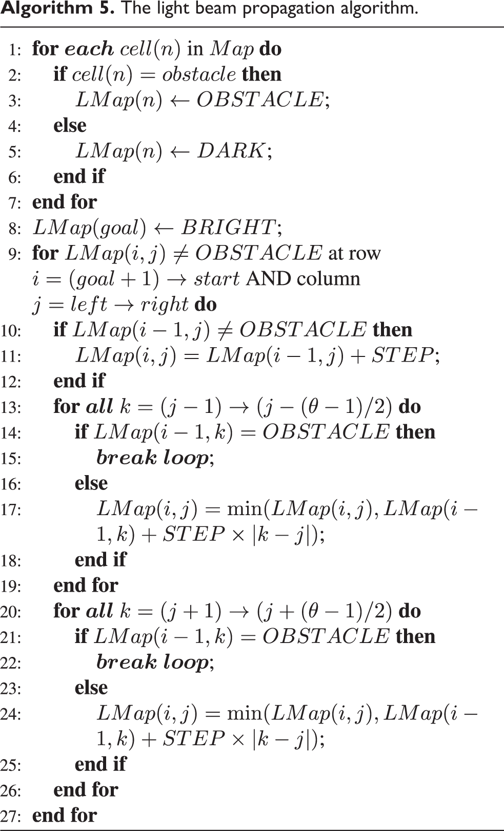
The light beam propagation algorithm is described in Algorithm 5. Firstly, all the nodes’ brightness value in the $L M a p$ are set to be DARK except the goal node’s brightness value which is set to be BRIGHT. Then the node’s brightness value is updated when the light beam propagates to the node. For example, θ is 3 in Figure 1(a), and the brightness value of node f can be calculated as

L M a p (n_{f}) = min_{i = a, b, c} [L M a p (n_{i}) + D i s t (n_{i}, n_{f})]

Algorithm 3.

$x_{min} \leftarrow C h o o s e P a r e n t (X_{k n e a r}, x_{n e w})$ .

Algorithm 4.

$T \leftarrow R e w i r e (T, x_{min}, X_{k n e a r}, x_{n e w})$ .

Algorithm 5.

The light beam propagation algorithm.

The brightness value of node f is equal to the brightness value of its predecessor node plus the distance which the light beam propagated. $L M a p (n_{f})$ is firstly set to be $L M a p (n_{b}) + S T E P$ (line 11 in Algorithm 5), then $L M a p (n_{f})$ will be updated if there is a smaller value exist (lines 17 and 24 in Algorithm 5). Note that, nodes a, b, and c have the same distance, which is equal to $S T E P \times 1$ , to node f as shown in Algorithm 5. This method of calculating distance is slightly different from Manhattan distance.

In the proposed P-RRT algorithm, Euclidean distance is adopted to calculate the propagation distance. Hence, the distance from nodes a and c to node f becomes $S T E P \times \sqrt{2}$ . In order to see the difference more clearly, the approximate counter map of brightness value is generated as shown in Figure 2(b). It is more reasonable to use Euclidean distance than the calculation method in LA* due to that the tree will grow toward the goal node more easily.

Phototropism RRT

Algorithm 6.

P-RRT algorithm.

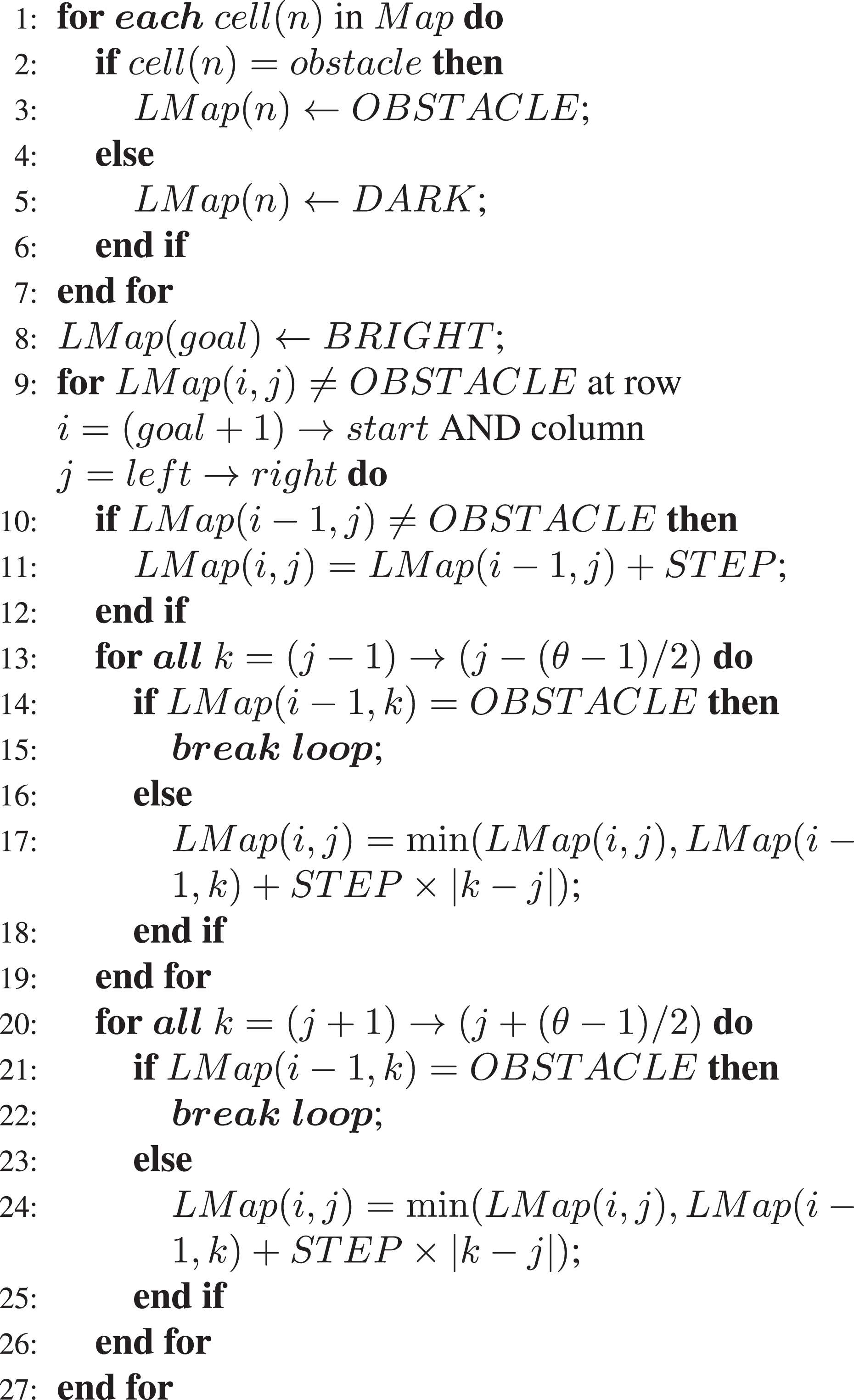
The P-RRT algorithm pseudocode is shown in Algorithm 6. There are some differences from the RRT algorithm. Initially, the P-RRT algorithm generates the light beam propagation map (line 1). Then the tree grows toward the light source, which is the goal node, on the light beam propagation map. The $S a m p l e ()$ and $N e a r e s t ()$ functions are just as the same as in RRT algorithm (lines 5 and 6). The $R e S a m p l e ()$ function is called to resample n random nodes around the node $x_{n e a r e s t}$ (line 8). As shown in Figure 3, a semicircle brightness detection area, which is facing to the node $x_{r a n d}$ , is generated with node $x_{n e a r e s t}$ as the center. In Figure 3, there are six nodes resampled in the brightness detection area and the node x ₂ with the minimum brightness value is chosen as node ${x^{'}}_{r a n d}$ . Then the $S t e e r ()$ function is called and returns a node $x_{n e w}$ (line 8). If the edge connecting $x_{n e a r e s t}$ and $x_{n e w}$ does not collide with any obstacle (line 9), the node $x_{n e w}$ and its corresponding edge $(x_{n e a r e s t}, x_{n e w})$ is added into the tree T (lines 10 and 11).

Figure 3.

Diagram of $R e S a m p l e ()$ function.

At last, the $A d j u s t S a m p l e S p a c e ()$ function is called to reduce the sample space in order to improve the sampling efficiency. The random node is sampled in the whole workspace at the first iteration process. Then the sample space will be adjusted in subsequent iteration process. As shown in Figure 4(a), node $x_{r 2}$ is an effective sampling node while node $x_{r 1}$ is not, and node $x_{n e w}$ is added into the tree T as described in Algorithm 6. If the brightness value of node $x_{n e w}$ is the minimum in the tree T, the sample space will be adjusted as shown in Figure 4(b). This will enable the $S a m p l e ()$ function to sample from the space which is better for the tree to grow toward the goal node. Note that, the P-RRT algorithm can still find a solution when the sample space is reduced. It is because that node $x_{n e w}$ is still under the light when the sample space is adjusted, thus there is a path, along which light beam propagates, exist between node $x_{n e w}$ and the goal node. In addition, if there is no node under the light at the first iteration process, the P-RRT will work as the same as the RRT algorithm until any node reach the light.

Figure 4.

Diagram of adjusting sample space: (a) Before adjusting and (b) after adjusting.

Although in the P-RRT algorithm, the tree grows toward the light source and the P-RRT’s path length is shorter than the RRT’s, there are redundant nodes on the P-RRT’s path due to the inherent randomness of the algorithm. When the P-RRT algorithm finds a path between the start node and the goal node, an optimization process, which is based on the concept of line of sight (LOS), is adopted to optimize the path. As shown in Figure 5, the P-RRT’s path is $A - B - C - D - E$ . The optimization process firstly tries to connect nodes A and E directly, which are the two end points of the path. Because of the path $A - E$ is blocked by the obstacle, then the optimization process tries to connect nodes A and D while keeping the path $D - E$ . The path $A - D$ is collision free, thus the final path is $A - D - E$ . The optimization process can also be seen as building a visibility graph. In order to distinguish with the result of P-RRT algorithm described above, P-RRT algorithm added the optimization process is called OP-RRT algorithm.

Figure 5.

Diagram of the optimization process.

Experiments

To test the proposed algorithm performance, RRT, RRT*, P-RRT, and OP-RRT are realized and tested in the same experimental environment which is developed by Matlab and runs on PC with 2.3 GHz CPU and 16 GB RAM. Two experiment scenarios are designed as follows.

Comparisons on scenario 1

In scenario 1, the map size is 406 × 710 (see Figure 6) and some obstacles are placed with random orientations across the map. The start node is located at the bottom of the map and the goal node is located at the top of the map. The angle θ is 23 which is proved that can provide the minimum possible overhead while maintaining zero probability of blocking light.²³ The performance of RRT, RRT*, P-RRT, and OP-RRT is compared by averaging the results of the 100 generated instances. Two groups of experiments are carried out. In the first group, all algorithms do not consider the non-holonomic constraints of mobile robot. In the second group, the non-holonomic of mobile robot is considered and realized by RRT and P-RRT which are noted by RRTu and P-RRTu, respectively. In all experiments, the velocity of the robot is 10 m/s.

Figure 6.

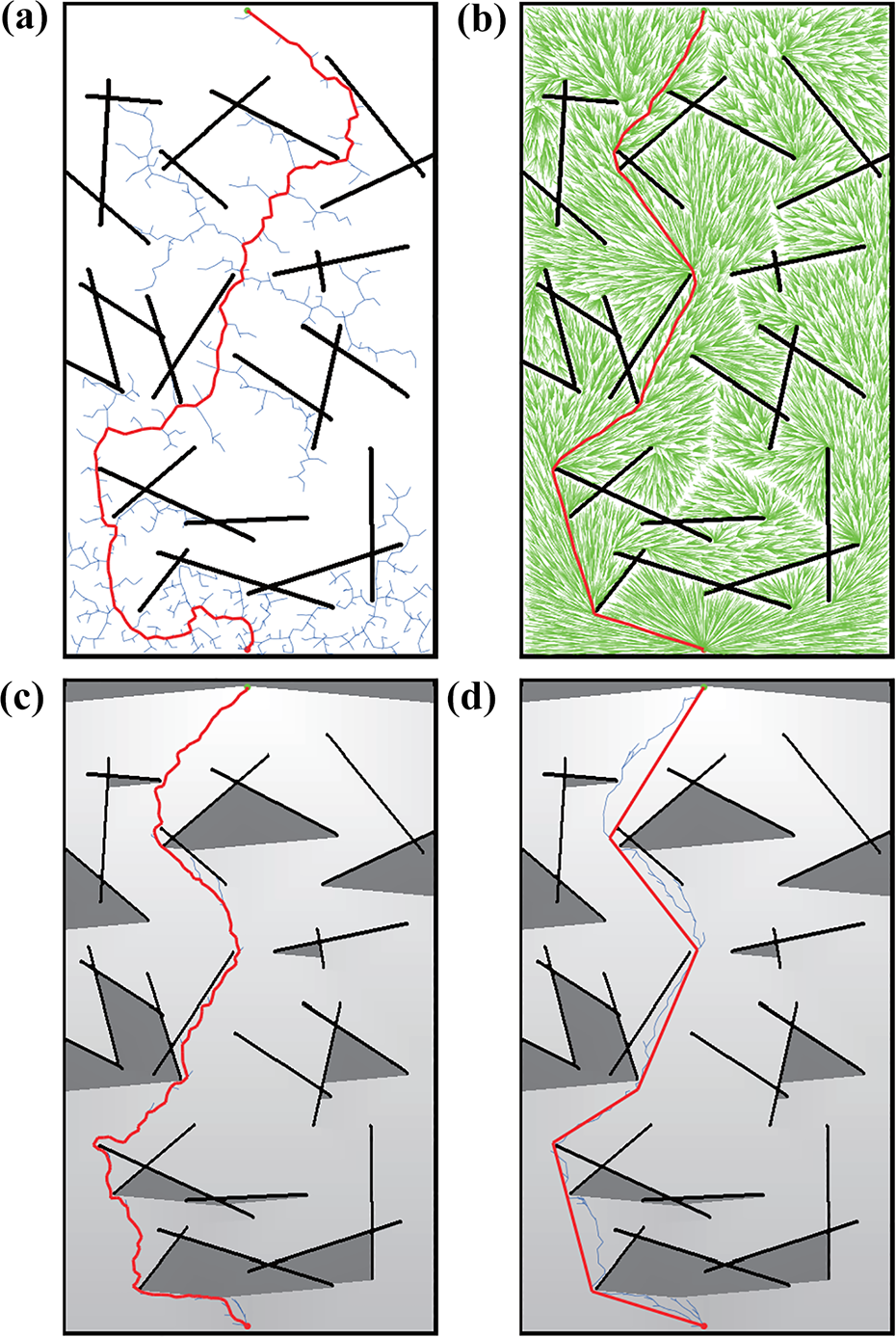
The comparison of RRT, RRT*, P-RRT, and OP-RRT in scenario 1. (a) Result of RRT (length = 1168.5 m, time = 314.8 ms), (b) result of RRT* (length = 906.5 m, time = 375.2e+3 ms), (c) result of P-RRT (length = 1026.2 m, time = 162.4 ms), and (d) result of OP-RRT (length = 910.2 m. time = 193.5 ms). RRT: rapidly exploring random tree; P-RRT: phototropism rapidly exploring random tree.

In the first group, the final planning paths of each algorithm in one experiment are shown in Figure 6. In RRT algorithm, the goal node is chosen as the sample node with probability of 0.05 which is a common skill for speeding up RRT algorithm to find the path. The final path of the RRT* is the result of 30,000 iterations (see Figure 6(b)). Although it takes a lot of computing resources to optimize the solution, RRT* only finds a suboptimal solution approaching to the optimal solution.

As shown in Figure 6(c) and (d), the map is lit up by the virtual light source which is set at the same place as the goal node on the top of the map. The dark regions in the map are the areas where the light beam cannot reach. Guiding by the light beam, the P-RRT algorithm can find the path in a shorter time than RRT algorithm while its final path is also shorter than RRT’s. As shown in Figure 6(d), OP-RRT algorithm firstly works as the same as the P-RRT algorithm and then optimizes the path based on the concept of LOS as described above. The path length of OP-RRT is quite close to the path length of RRT* and the OP-RRT algorithm takes quite smaller computation cost than RRT* algorithm. Due to the inherent randomness and additional optimization process, OP-RRT algorithm takes a little bit more computation cost than P-RRT algorithm.

The statistical results of each algorithm are shown in Table 1. The node number of RRT* is the largest one due to that RRT* algorithm takes a lot of time to optimize the connection of the tree. It needs more memory to maintain such a big tree structure. The node number of RRT algorithm is the second one. P-RRT algorithm and OP-RRT algorithm use the same grow strategy proposed in this article, thus they have the similar minimum node number.

Table 1.

The comparison in scenario 1 without non-holonomic constrain.

	RRT	RRT*	P-RRT	OP-RRT
Avg nodes	1572.1	26,143	225.9	226.0
Max nodes	4281	26,419	305	299
Min nodes	714	25,594	184	180
Avg time (ms)	445.7	381.2e+3	118.1	193.0
Max time (ms)	1.1e+3	394.5e+3	676.7	705.1
Min time (ms)	151.1	365.5e+3	60.8	99.1
Avg length (m)	1293.9	906.3	1025.1	906.9
Max length (m)	1487.5	914.0	1068.6	921.3
Min length (m)	1164.1	901.5	991.4	897.3

RRT: rapidly exploring random tree; P-RRT: phototropism rapidly exploring random tree.

In Table 1, the computation cost of the RRT* is also the largest one due to it takes more time to extend a node as the total nodes of tree become large. In scenario 1, it takes nearly 400 s on average to execute 30,000 iterations. RRT algorithm expands a lots of nodes which are not good for the tree grows toward the goal due to there are “trap” areas in scenario 1. This led to RRT algorithm that takes 445.7 ms on average to find the solution. In contrast to that, the proposed algorithm utilizes the $L M a p$ to optimize the sample process so that the tree will extends its branches to the areas where the brightness value decreases and avoids the “trap” areas at the same time. Therefore, the computation cost of the proposed algorithm is lower than RRT algorithm. Note that, the computation cost of generating the $L M a p$ is shown in Table 2, and the statistical results are based on running $L M a p$ function 100 times. The maximum and average time are 19.1 and 15.1 ms, respectively, which compared with the computation cost of main process is relatively small. Thus, the main computation cost of P-RRT and OP-RRT is still the growth of the tree.

Table 2.

The computation cost to generate the $L M a p$ in scenario 1.

	Avg time	Max time	Min time
$L M a p$	15.1 ms	19.1 ms	13.9 ms

The average path length of RRT* is the shortest in all comparison algorithms and the result still has room for optimization as long as it continues to iteration. In contrast to that, the average path length of RRT is the longest in all comparison algorithms. Compared with RRT algorithm, P-RRT algorithm can shorten the average path length by 20.8% due to the $L M a p$ can guide the growth direction of the tree. By using the optimization process of LOS, OP-RRT algorithm can further shorten the average path length by 9.1%.

In the second group, the final planning paths of each algorithm in one experiment are shown in Figure 7. The statistical results of 100 times experiments are shown in Table 3. When considering the non-holonomic constrain, the random sample node is hard to be a valid expand node. Accordingly, RRTu and P-RRTu both take more computation memory and time to find the solution. Hence, the runtime of this group of experiments is measured in seconds and it is the same in scenario 2. To further test the performance, the maximum number of tree nodes is set to be 10,000. If the number of nodes reaches the maximum number, the algorithm stops immediately and is treated as failure to find the solution in this experiment. As shown in Table 3, the success rate of RRTu and P-RRTu is 88% and 98%, respectively. P-RRTu algorithm has a higher success rate due to the $L M a p$ improves the effective of the sample node. At the same time, the other indexes of P-RRTu are also better than RRTu.

Figure 7.

The comparison of RRTu and P-RRTu in scenario 1. (a) Result of RRTu (length = 1333.3 m, time = 2.7 s) and (b) result of P-RRTu (length = 1072.0 m, time = 2.0 s). RRT: rapidly exploring random tree; P-RRT: phototropism rapidly exploring random tree.

Table 3.

The comparison in scenario 1 with non-holonomic constrain.

	RRTu	P-RRTu
Avg nodes	5359.7	2579.6
Max nodes	11,688	9452
Min nodes	1790	656
Avg time (s)	2.4	1.7
Max time (s)	5.6	4.8
Min time (s)	0.8	0.3
Avg length (m)	1266.9	1055.6
Max length (m)	1487.7	1104.4
Min length (m)	1044.2	1019.6
Success rate	88%	98%

Comparisons on scenario 2

In scenario 2, the map size is 160 × 320 (see Figure 8) and n square-shaped obstacles are placed at random locations throughout the map. The start node is located at the bottom right corner of the map and the goal node is located at the top left corner of the map. In this scenario, several maps are randomly generated according to the gradual increase of obstacles. The performance of RRT, RRT*, P-RRT, and OP-RRT is compared by averaging the results of the 100 generated instances in each map. Two groups of experiments are carried out as same as in scenario 1.

Figure 8.

The comparison of RRT, RRT*, P-RRT, and OP-RRT in scene 2 (500 obstacles). (a) Result of RRT (length = 271.2 m, time = 54.8 ms), (b) result of RRT* (length = 232.0 m, time = 110e+3 ms), (c) result of P-RRT (length = 269.2 m, time = 35.7 ms), and (d) result of OP-RRT (length = 243.9 m, time = 57.1 ms). RRT: rapidly exploring random tree; P-RRT: phototropism rapidly exploring random tree.

As shown in Figure 8, this is the case of 500 obstacles randomly placed in the map. The statistical results of 100 times experiments are shown in Table 4. RRT* algorithm has the shortest average path length while it has the most average nodes and computation cost. P-RRT and OP-RRT have the similar minimum nodes due to the same reason as described above. The computation cost of P-RRT is the minimum. There are no “trap” areas in scenario 2, thus the sampling efficiency of RRT algorithm is increased. But it still takes more computation memory and cost than P-RRT and OP-RRT on average. The path length of OP-RRT is shorter than P-RRT, but the computation cost is higher than P-RRT. Note that, the maximum time of OP-RRT is relatively high. In scenario 2, the LOS process sometimes takes long time to optimize the path due to there are a lots of random obstacles which have high probability of blocking the LOS. Hence, it increases the processing time.

Table 4.

The comparison in scenario 2 without non-holonomic constrain (500 obstacles).

	RRT	RRT*	P-RRT	OP-RRT
Avg nodes	235.5	6823.4	54.8	52.6
Max nodes	823	7022	77	75
Min nodes	63	6704	45	40
Avg time (ms)	64.1	113.8e+3	46.0	60.1
Max time (ms)	271.5	126.7e+3	103.8	301.9
Min time (ms)	26.2	109.8e+3	21.1	22.7
Avg length (m)	327.5	233.7	284.4	255.6
Max length (m)	454.3	236.0	296.0	280.4
Min length (m)	266.1	231.7	259.2	238.5

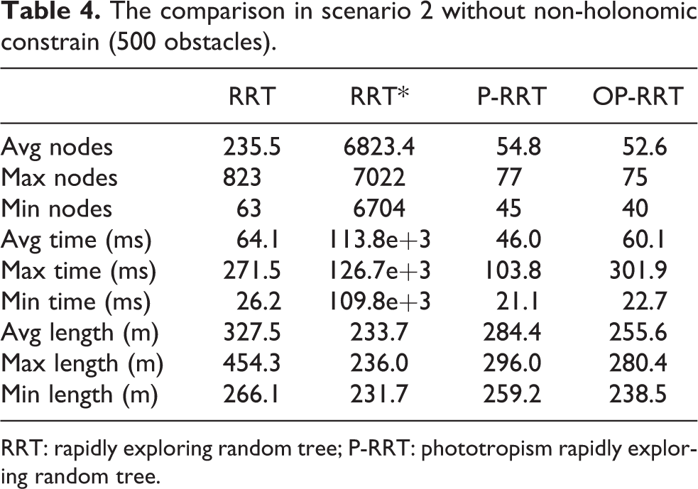
RRT: rapidly exploring random tree; P-RRT: phototropism rapidly exploring random tree.

The computation cost of generating the $L M a p$ is shown in Table 5, and the statistical results are based on running $L M a p$ function 100 times. The results still relatively small compared to the main processing flow.

Table 5.

The computation cost to generate the $L M a p$ in scenario 2 (500 obstacles).

	Avg time	Max time	Min time
$L M a p$	1.5 ms	4.5 ms	1.3 ms

In the second group, the final planning paths of each algorithm in one experiment are shown in Figure 9. The statistical results of 100 times experiments are shown in Table 6. In terms of each index, the performance of P-RRTu is better than RRTu. Note that, the success rate of RRTu is very low which will be analyzed below.

Figure 9.

A comparison of RRTu and P-RRTu in scenario 2. (a) Result of RRTu (length = 383.2 m, time = 6.7 s) and (b) result of P-RRTu (length = 280.2 m, time = 1.6 s).

Table 6.

The comparison in scenario 2 with non-holonomic constrain (500 obstacles).

	RRTu	P-RRTu
Avg nodes	9817.8	3662.9
Max nodes	19,420	9694
Min nodes	765	430
Avg time (s)	5.8	2.8
Max time (s)	16.1	8.3
Min time (s)	0.4	0.2
Avg length (m)	359.5	291.2
Max length (m)	500.5	338.0
Min length (m)	286.5	254.3
Success rate	48%	99%

The performance profile in the case of different number of obstacles in scenario 2 without non-holonomic constrain is shown in Figure 10. All results are the average of 100 generated instances. Note that, the results of RRT* algorithm are not drawn on the graph due to the computation cost is much larger than other algorithms. As shown in Figure 10(a), the node number of RRT algorithm increases with the number of obstacles. The node number of P-RRP and OP-RRT have barely increased because of the $L M a p$ can guide the tree grow effectively. When the number of obstacles is less than 400, the CPU runtime of the three algorithms is almost similar. As obstacles continue to increase, CPU runtime of the three algorithms begin to increase. RRT algorithm is the most obvious one. OP-RRT algorithm also has a small increase because of that the computation cost of LOS process increases. When there are many obstacles in the map, the efficiency of LOS process will be greatly reduced. Although the final path length of the three algorithms all grow slightly, the results of OP-RRT algorithm are always the shortest. From this set of experimental data, it can be seen that OP-RRT algorithm trades time for a shorter path than P-RRT algorithm, but with the increase of obstacles, the cost will become less cost-effective.

Figure 10.

The performance profile in the case of different number of obstacles in scenario 2 without non-holonomic constrain. (a) Node number, (b) CPU runtime, and (c) path length.

The performance profile in the case of different number of obstacles in scenario 2 with non-holonomic constrain are shown in Figure 11. As shown in Figure 11(a) and (b), the computation memory and time of the two algorithms both increase with the increase of obstacle. The increment of P-RRTu algorithm is smaller than that of RRTu algorithm. The path length of P-RRTu algorithm increases very small with the increase of obstacle. The increase of obstacle makes the path length of RRTu become longer and reduces the effectiveness of sampling nodes. Therefore, the success rate of RRTu algorithm is relatively low. When the number of obstacles exceeds 500, the success rate of RRTu drops sharply. In contrast, when the number of obstacles exceeds 700, the success rate of P-RRTu algorithm is reduced to less than 50%.

Figure 11.

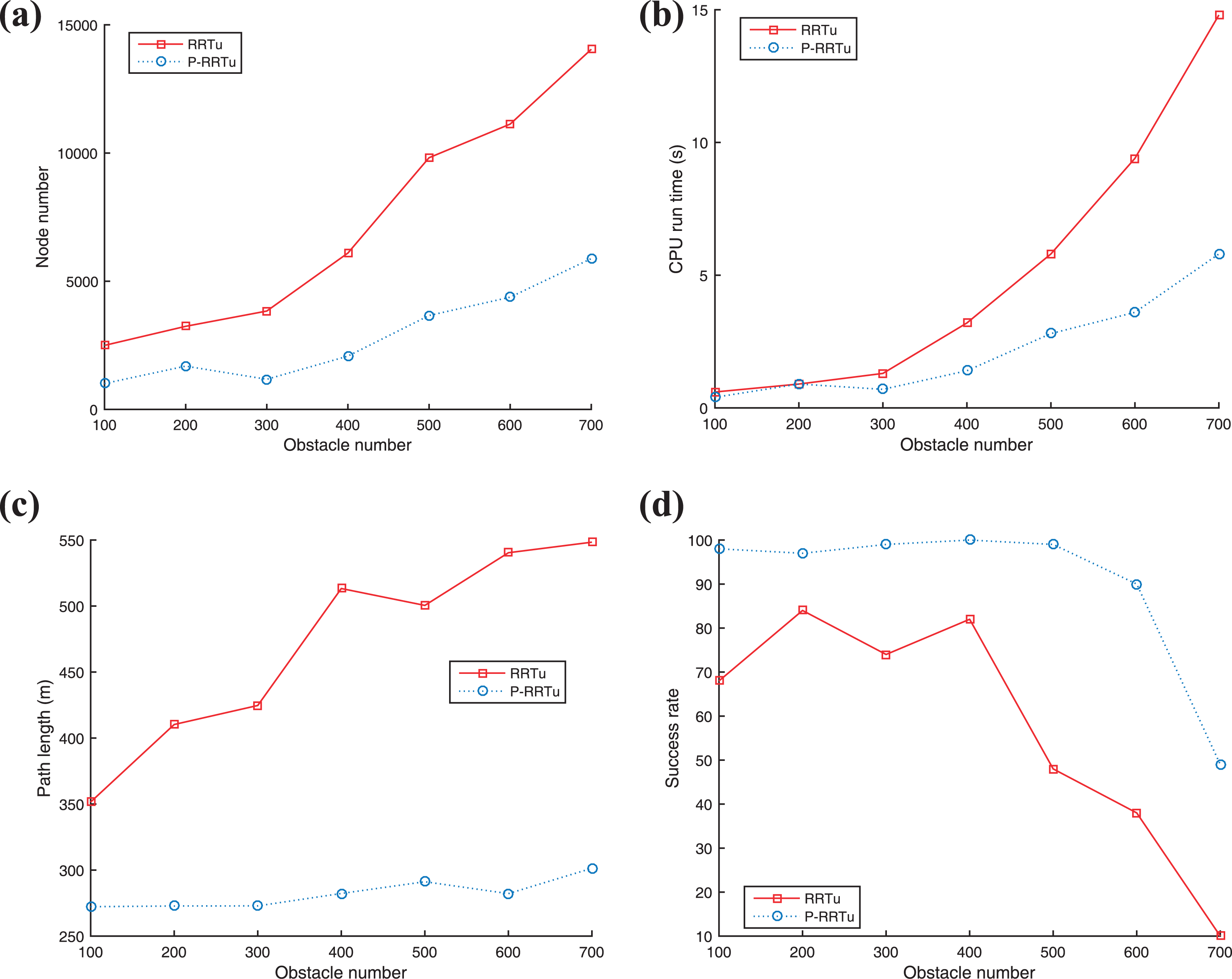
The performance profile in the case of different number of obstacles in scenario 2 with non-holonomic constrain. (a) Node number, (b) CPU runtime, (c) path length, and (d) success rate.

Results of different distance functions

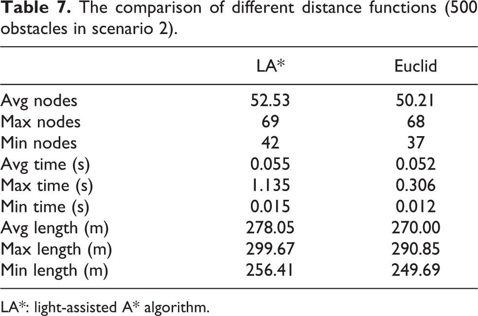
As described in the above section, the propagation distance calculated by different distance functions will influence the path along which light propagate. This will also influence the growth of the P-RRT. As shown in Figure 12, P-RRT grows toward the light source more easily when using the Euclidean distance. The statistical results of 100 times experiments are shown in Table 7. The results show that P-RRT with the Euclidean distance has better performance than with LA* distance.

Figure 12.

The results of different distance functions in scene 2 (500 obstacles). (a) LA* distance and (b) Euclidean distance. LA*: light-assisted A* algorithm.

Table 7.

The comparison of different distance functions (500 obstacles in scenario 2).

	LA*	Euclid
Avg nodes	52.53	50.21
Max nodes	69	68
Min nodes	42	37
Avg time (s)	0.055	0.052
Max time (s)	1.135	0.306
Min time (s)	0.015	0.012
Avg length (m)	278.05	270.00
Max length (m)	299.67	290.85
Min length (m)	256.41	249.69

LA*: light-assisted A* algorithm.

Conclusions

In this article, an improved RRT algorithm which is inspired by the phototropism of plants is proposed. A virtual light source is set at the goal node to light up the whole map. The lighted map, which is called $L M a p$ , is treated as the heuristic information. In the $L M a p$ , the lower is the brightness value, the higher is the actual light intensity value. Therefore, the explore tree extends its branches toward the areas with high light intensity value like a real plants. The sampling efficiency is improved by designing the resample function and adjusting the sample space. The results of experiments show that the P-RRT algorithm can effectively reduce the cost of computing memory and time. The path length of P-RRT is also shorter than the RRT algorithm.

The optimization process, which is based on the concept of LOS, is used to further shorten the path length. Although the computation time is increased, the path length obtained by OP-RRT algorithm is very close to the approximate optimal solution of RRT* algorithm which is obtained by consuming a lot of computing resources. The results of experiments show that the optimization effect is better when the number of obstacles is relatively small. The results of experiments also show that the time of optimization process is increased significantly with the further increase of obstacles. When considering the non-holonomic constraint of the mobile robot, the proposed algorithm can still improve the sampling efficiency and guide the growth of the explore tree to ensure a high success rate to find the solution.

Footnotes

Acknowledgement

The authors would like to thank the referees for their comments.

Declaration of conflicting interests

The author(s) declared no potential conflicts of interest with respect to the research, authorship, and/or publication of this article.

Funding

The author(s) disclosed receipt of the following financial support for the research, authorship, and/or publication of this article: This work was supported by Natural Science Foundation of Zhejiang Province (LQ18F030013, LQ18F030014).

ORCID iD

Chengchen Zhuge

References

Sedighi

Nguyen

Kapsalas

, et al. Implementing Voronoi-based guided hybrid A* in global path planning for autonomous vehicles. In: 2019 IEEE intelligent transportation systems conference (ITSC), Auckland, New Zealand, 27–30 October 2019, pp. 3845–3852.

Geraerts

. Planning short paths with clearance using explicit corridors. In: IEEE international conference on robotics & automation, Anchorage, AK, USA, 3–7 May 2010.

Qiu

Chen

. A hybrid two-dimensional path planning model based on frothing construction algorithm and local fast marching method. Comput Electr Eng 2013; 2: 475–487.

Aarno

Kragic

Christensen

. Artificial potential biased probabilistic roadmap method. In: 2004 IEEE international conference on robotics and automation, New Orleans, LA, USA, 26 April–1 May 2004, pp. 461–466. IEEE.

Yan

Zhang

Wang

. Path planning for mobile robot’s continuous action space based on deep reinforcement learning. In: 2018 international conference on big data and artificial intelligence (BDAI), Beijing, China, 22–24 June 2018, pp. 42–46.

Sichkar

. Reinforcement learning algorithms in global path planning for mobile robot. In: 2019 international conference on industrial engineering, applications and manufacturing (ICIEAM), Sochi, Russia, 25–29 March 2019, pp. 1–5.

Santiago

RMC

De Ocampo

Ubando

, et al. Path planning for mobile robots using genetic algorithm and probabilistic roadmap. In: 2017 IEEE 9th international conference on humanoid, nanotechnology, information technology, communication and control, environment and management (HNICEM), Manila, Philippines, 1–3 December 2017, pp. 1–5. IEEE.

Huh

Lee

. Learning high-dimensional mixture models for fast collision detection in rapidly-exploring random trees. In: 2016 IEEE international conference on robotics and automation (ICRA), Stockholm, Sweden, 16–21 May 2016, pp. 63–69. IEEE.

Connell

Manh La

. Extended rapidly exploring random tree–based dynamic path planning and replanning for mobile robots. Int J Adv Robot Syst 2018; 15: 1729881418773874.

10.

Khatib

. Real-time obstacle avoidance for manipulators and mobile robots. In: Cox

Wilfong

(eds) Autonomous robot vehicles, New York: Springer, 1986, pp. 396–404.

11.

Zuo

Guo

, et al. A hierarchical path planning approach based on A* and least-squares policy iteration for mobile robots. Neurocomputing 2015; 170: 257–266.

12.

Plaza

Martnez-Marn

Prieto

, et al. Integration of cell-mapping and reinforcement-learning techniques for motion planning of car-like robots. IEEE Trans Instrum Meas 2009; 58: 3094–3103.

13.

Zivojevic

Velagic

. Path planning for mobile robot using Dubins-curve based RRT algorithm with differential constraints. In: 2019 international symposium ELMAR, Zadar, Croatia, 23–25 September 2019, pp. 139–142.

14.

LaValle

Kuffner

. Rapidly-exploring random trees: Progress and prospects. Algorithmic and Computational Robotics: New Directions 2001; 5: 293–308.

15.

Kuffner

LaValle

. RRT-connect: an efficient approach to single-query path planning. In: Proceedings 2000 ICRA. Millennium conference. IEEE international conference on robotics and automation symposia proceedings, San Francisco, CA, USA, 24–28 April 2000, pp. 995–1001. IEEE.

16.

Karaman

Frazzoli

. Sampling-based algorithms for optimal motion planning. Int J Robot Res 2011; 30: 846–894.

17.

Nasir

Islam

Malik

, et al. RRT*-SMART: a rapid convergence implementation of RRT. Int J Adv Robot Syst 2013; 10: 299.

18.

Conte

Zulli

. Hierarchical path planning in a multi-robot environment with a simple navigation function. IEEE Trans Syst Man Cybern 1995; 25: 651–654.

19.

Lulu

Elnagar

. A comparative study between visibility-based roadmap path planning algorithms. In: 2005 IEEE/RSJ international conference on intelligent robots and systems, Edmonton, Alta, Canada, 2–6 August 2005, pp. 3263–3268.

20.

Solovey

Salzman

Halperin

. Finding a needle in an exponential haystack: discrete RRT for exploration of implicit roadmaps in multi-robot motion planning. In: Algorithmic Foundations Robot XI. Cham: Springer, 2015, pp. 591–607.

21.

Qureshi

Ayaz

. Intelligent bidirectional rapidly-exploring random trees for optimal motion planning in complex cluttered environments. Robot Auton Syst 2015; 68: 1–11.

22.

Véras

Medeiros

Guimaraes

. Rapidly exploring random tree* with a sampling method based on Sukharev grids and convex vertices of safety hulls of obstacles. Int J Adv Robot Syst 2019; 16(1): 1729881419825941.

23.

Hawa

. Light-assisted A* path planning. Eng Appl Artif Intell 2013; 26: 888–898.