Sage Journals: Discover world-class research

Abstract

The online monitoring of water environments is urgently needed. A feasible and effective approach is the use of agents. Water environments, similar to other real-world environments, present many changing and unpredictable situations. To ensure flexibility in such an environment, agents should be prepared to deal with various situations. In this study, we focused on an adaptive agent tracking approach for oil contamination. An integrated tracking framework, which is used to track the moving contour of oil pollution via a system comprising multiple unmanned surface vehicles, is proposed. The zigzag, unmanned underwater vehicle-gas, cloverleaf trajectory and curvature-weighted deployment algorithm methods are employed with consideration of their suitability to our approach. A cyclic particle swarm optimisation–Kalman method is also proposed. The possible position of moving vertices is predicted by the Kalman filter, and an objective search region is generated around the centre position. Moreover, particle swarm optimisation is performed to search for the best target position in this region. This particle swarm optimisation–Kalman method is circle operated to compensate for the deficiency of a few agents. To evaluate the approach, we conduct usability and performance simulations.

Keywords

Agent tracking oil contamination water environment adaptive

Introduction

Sudden water pollution accidents, such as the leakage accident in the Mexico gulf crude oil drilling platform in April 2010, the oil spill accident in the Bohai Gulf oil field in June 2011 and the oil spill caused by the collision of an Iranian oil tanker in the East China Sea in 2018, occur frequently. Such occurrences pose a severe threat to the ecological environment. Failure to take timely and effective measures would result in inestimable losses. We must monitor the spread range and the trace of pollution following water pollution accidents. An accurate prediction is critical for taking the proper measures to minimise the extent of losses. However, the complexity of water environments makes monitoring difficult. For example, monitoring is affected by flow field, wind field, clouds or fog that are present in water environments. With the development of artificial intelligence technology, autonomous mobile agents which are equipped with multiple sensors have been increasingly applied to environmental monitoring, disaster relief, military exploration and other tasks.^1

–4 The employment of multi-agent for water pollution monitoring is a complex issue because water pollution is nonstatic and it expands and drifts with flow. The major problem is the tracking of mobile targets by multiple, cooperative, mobile agents in an unknown dynamic environment. In this study, we focus on a cooperative method involving multi-agent to track the spatial distribution and trail of oil contamination in water. Based on the existing studies, this study proposes a complete approach that covers pollution plume exploration, contamination confirmation, contour detection and dynamic tracking. The motion of oil contamination on the water surface is discussed, and the monitoring objectives of the multi-agent approach are determined. To discover the plume of oil contamination, we use the zigzag method in searching for pollution information and the cloverleaf trajectory method in confirming continuous large-scale oil contamination. Meanwhile, the unmanned underwater vehicle (UUV)-gas method is used to detect the contour of the contamination and determine its spatial distribution. Next, multiple unmanned surface vehicles (USVs) are distributed along the contour of the contamination according to the curvature-weighted deployment algorithm (CDA). Finally, the cyclic particle swarm optimisation–Kalman (CPK) method is proposed to track dynamic contamination. In this method, the possible position of moving vertices is predicted by the Kalman filter, and a search region is generated around the centre position. Particle swarm optimisation (PSO) is utilised to search the best target point position in the region. To make up for the deficiency of few agents, we operate the CPK method in a circular manner along the contour.

Related work

References review

Recent advances have been made in the estimation of the spatial distribution and tracking of pollution clouds. The existing studies^5
–7 adopt numerical simulation methods to simulate the oil spill drift–diffusion process. The approach tends to build an exact model which should be verified by a large amount of data. Weiping Cheng et al. proposed a pollution cloud’s spatial reconstruction model based on the backward probability density function. The direct scanning method was used to search the optimal solution.⁸ The contamination transmission model is required in this method. On the basis of a diffuse model of the measurement generation process, Gilholm and Salmond proposed a different approach for the extended object problem, in which the target is represented by a spatial probability distribution.⁹ This probabilistic method is based on various numerical analysis algorithms, such as the Gaussian feather, Lagrangian transport and Eulerian transport models. The methods mentioned are used mostly in the reversal tracing of pollution source. Both of these methods need mass of numerical data. In the condition of lack of priori knowledge of environment and pollution, the numerical method and other algorithms based on it seems inapplicable.

Recently, a study on the autonomous robotic system has gained popularity in various fields.¹⁰ Vitor et al.¹¹ give a detail survey on agent for disaster which include robotics disaster management, general surveys regarding agents, navigation, higher level autonomy, structure inspection and environmental monitoring. Most autonomous agents are designed to operate in oceans, rivers and lakes. For example, autonomous agents were designed for spatial measurements in rivers and coastal reconnaissance,^12,13 and autonomous surface vehicles were constructed for oil skimming and clean-up.¹⁴ Nevertheless, in water environments, using a single agent for target detection is not enough because of the wide range of working space and other limitations. These limitations include the following. (1) The lack of global information results in the vulnerability of the exploration process to false-alarmed sensor information, changed environmental information and other factors, which may lead to poor decision-making, poor exploration efficiency and prolonged exploration time. (2) A single agent may fall into local extreme values due to the limited environmental information available, resulting in misjudgement. (3) Once the single agent fails, the task cannot be completed.

For these reasons, increasing attention has been paid to the theory and technology of multi-agent.^10,15
–17, Compared with a single agent, a multi-agent system has some merits. Firstly, it can obtain a satisfactory spatial distribution and working performance. Secondly, a multi-agent system that uses a certain number of simple, inexpensive agents is less costly than a single, complex and expensive agent. Finally, such system has better reliability, flexibility, scalability and versatility than a single agent does.¹⁸ Agents with different abilities can collaborate to accomplish complex tasks; even if one or more agents fail, task completion is not affected.

The study of advanced, distributed artificial intelligence techniques in developing a cooperative multi-agent system that is oriented to support environmental monitoring applications has gained considerable attention. Traditional research was inclined to build sensor networks composed of several sensors which are independent and distributed and able to collect information on the ground. The collected information is transferred to a central system for processing to return high-level indications who can take operative decisions.¹⁹ However, this method requires numerous perceptive sensors which are motionless and difficult to maintain. Cooperative multi-agent systems, such as unmanned ground vehicles, unmanned air vehicles (UAVs), UUVs or USVs, have been shown to be superior to sensor networks because of their techniques that are based on artificial intelligence in the environmental monitoring domain. In such a way, perceptive agents are allowed not only to adapt their measurement capabilities to the changing environmental conditions but also to cooperate in gathering information and making intelligent decisions.

Some algorithms have been developed to monitor contaminant scope, for example, the snakes and UUV-gas algorithms.²⁰ On the one hand, snakes were originally developed for image segmentation, the goal of which is to find a structure inside a noisy 2D image. A snake is a curve that quickly wraps itself around a structure when placed near it. On the other hand, the UUV-gas algorithm treats vehicles as a gas of particles affecting one another’s speed. When the UUV is inside the perimeter, it turns clockwise; when it is outside, it turns counterclockwise. The route of UUVs is snake-like.

Trincavelli et al. proposed a topological map for contamination cloud monitoring by multi-UAV. The frontier points of a contamination cloud detected by the multi-UAV were regarded as feature points, which were linked by curves with a fix curvature. The 2D boundary curve of the contamination cloud was built. Thereafter, a 3D environment model was derived by stacking 2D models in different altitudes. This method is intuitionistic and compact and is thus convenient for data exchange monitoring among multi-UAV; it also makes the cooperative control and navigation algorithm effective.²¹

However, these studies did not consider the dynamic characteristics of contamination. Water environment is dynamic. The contamination in water has varying scope and contour which are influence by wind, flow obstacle and other factors. Agents should have the ability to adapt their measurement capabilities to changing environmental conditions.

Kato et al. describe a project regarding detection of gas and oil spills.^22,23 In this project, they perform autonomous tracking and monitoring of spilled plumes of oil and gas. Fahad et al. present a simulation of a single robot that performs oil plume tracking.²⁴ This simulation aims to perform the validation of the controller as well as to test the robustness of the control using complex probabilistic environmental models. The studies mainly focus on the tacking algorithm of the spilled plumes of oil and gas but not mention the monitoring method for dynamic scope and contour of spilled oil.

The authors in the literature^25

–28 studied an algorithm for tracking moving objects. Hu and Xu proposed an approach to real-time tracking of moving objects that is based on the genetic algorithm (GA) and Kalman filter. In their work, the possible position of a moving target’s centre in the next image was predicted by a Kalman filter, and a target search region was generated around the centre position. GA was utilised to search for the best position which has the best GA fitness function calculate result in the search region.²⁹ These studies exhibited effectiveness and robustness in dynamic target tracking, but they are still limited in terms of contamination contour tracking. Firstly, most of these methods are based on the prerequisite of acquisition and pattern recognition of whole image regions of targets. However, in contamination contour tracking, a single USV cannot obtain the whole image or concentration field of the contamination. Secondly, the contamination contour extends when it drifts with flow. Moreover, the contour may not be continuous.

Contributions

The main contribution of this work is an algorithmic solution to the autonomous deployment of USVs which are used for oil contamination tracking in a flow environment. This algorithm can be used as a high-level routine for the tracking of USVs in cooperative surveillance or sensing tasks. We encode this objective through the performance metrics if agents lose tracked targets or if the mean error on the estimated contamination area within a selected time is considerably large. Most of the existing studies focus on the³⁰ tracing of a chemical plume to its source and declaring the source location. Although some methods are learned and used in our tracking flow, the research target is different. The tracked contamination in this study is widespread and dynamic and is thus impossible for a single agent to complete. Moreover, the track-in and track-out plume behaviour²⁰ cannot facilitate the estimation of the full extent of the contamination. Thus, we focus on the robotic tracking approach which has a complete working flow that covers pollution plume exploration, contamination confirmation, contour detection and dynamic tracking. In this approach, the cooperation of multiple agents is important. Additionally, estimation and prediction are inevitable. Although the existing studies study the algorithm for moving^27
–29 object tracking, it only involves point tracking. Therefore, we extend the relative method to the prediction of a large-scale moving contamination and combine it with the autonomous tracking algorithm of multi-USV.

Problem statement

Dynamic feature of oil contamination

Oil spill pollution is the monitored object in this study. Tracking a moving oil contamination is difficult, and therefore, the motion of oil contamination should be discussed first.

Oil films could be regarded as a circular diffusion on the water surface without the effects of wind and water flow. However, the movement of oil contamination could be influenced by a weak wind and water flow. Moreover, the diffusion feature of oil contamination is a typical factor which influences its spread range.³¹

Fay³² proposed a theory to divide the extension of oil films into four stages: inertial, viscous expansion, surface tension expansion and maintenance. For convenience, we simplify the motion process of oil films as diffusion and drift stages. The spread covers the dominant position in the initial stage,³³ whereas drift is the main motion of oil contamination.

In the diffusion stage, the oil film drifts and expands with the flow. The expansion of the oil film surface will not stop until the end of the diffusion stage. Therefore, the scope of the oil film is a circle which continues to expand and move in the diffusion stage.

After the diffusion stage, the diameter of the oil film remains nearly constant. The area of the oil film could be calculated by³²

A_{f} = 10^{4} V^{3 / 4}

where V is the total volume of the oil film.

The above analysis shows that the oil contamination forms a continuous oil film on the water surface and moving with flow.

Design of the multi-USV system

Physical structure of single USV

To monitor oil pollution in a water environment, we design a multi-USV system in this study. The key components of the USV, which consists of a controller, some sensors and motor driver, GPS, collision avoidance, power, communication and directional modules, are shown in Figure 1.

Figure 1.

Components of the USV system. USV: unmanned surface vehicle.

The controller is the unit that executes the control algorithm and is responsible for the execution of the other modules. The USV has two propellers which are driven by two direct current motors. An ‘L289N’-driven board is used to produce pulse width modulation (PWM) signals to control the motor speed. Two motors help the USV to move forward or backward with a set speed and to turn in place. A GPS is used to detect the location of the USV. The directional module, which consists of a compass and a horizontal sensor, monitors the direction of the USV and feedbacks the signals to the controller. Meanwhile, the obstacle avoidance module detects obstacles through an infrared photoelectric sensor. The USV carries an oil sensor to detect oil films in water, which could be detected by the ultraviolet fluorescence spectrometric method.

Topological logic for cooperative decision-making of multiple USVs-remote centre

As shown in Figure 2, it is the communication link and collaborative decision-making topology diagram of multiple USVs-remote centre.

Figure 2.

Communication link and cooperative decision topology diagram of USV-remote monitoring centre. USV: unmanned surface vehicle.

The USV is equipped with short-range communications equipment to make accurately distance detect and formation maintenance (maintain suitable distance between USVs in formation). Considering that the limited communication distance between multiple USVs, when they are far away from each other, they are liable to fail to communication, and therefore, the telecommunication equipment is also equipped. In addition, due to the limited computing ability of the USV, a lot of complex computing consumes its energy and delays the detection time. Therefore, the remote centre undertakes the computing task and makes decisions on the cooperative behaviour of the USVs. The communication between USVs is limited to distance calculation and formation maintenance. As shown in Figure 2, the remote centre includes cloud server and remote monitoring centre. In which, cloud server receives data transmitted by USV and processes and stores the data. Meanwhile, the cloud server provides the decision-making for USVs’ cooperative behaviour and sends the decision command to the USV. The current 4G technology guarantees the communication rate between the USV and the remote centre. Even if a large amount of data is transmitted, it will not delay. The remote monitoring centre can issue monitoring tasks, check monitoring data and monitor the implementation of tasks.

In some cases, USVs need to form formations to accomplish certain tasks, for example, the pollution information search. Distributed control method based on artificial potential field and virtual leader for formation keeping among multiple USVs are adopted.³⁴ It keeps a suitable distance between USVs and keeps them from collision.

Purpose of this study

Tracking oil contamination is a dynamic target tracking problem. The tracked contamination usually has a large area and continues to spread and drift with flow. In some cases, its contour is discontinuous because of the distraction of turbulent flow, which can reduce the effectiveness and robustness of the tracking work. Considering the limitation of a single USV, we design a multi-USV system in this study. However, the tracking methodology for dynamic oil contaminations still requires further study. Although the robotic tracking method has been studied in the literature,^26

–29 the research into the tracking method for large dynamic oil contaminations is limited. The purpose of the current study is to propose a method for contamination monitoring and tracking via multi-USV. The dynamic feature of the tracked target should be considered in the method. Hence, the tracking algorithm of multi-USV should adapt to the changing environmental conditions while maintaining its effectiveness and robustness.

Materials and methods

A USV is utilised to track oil contamination on the water surface, detect the spread and drift status of pollutants, monitor the impact of pollution on the environment and assist waste-cleaning ships to clean water pollution. According to the four-stage behaviour pattern proposed by Wei Li et al.,³⁰ we define the following behavioural processes for the monitoring mission: searching for oil pollution information, tracing the contour that determines the scope, predicting and tracking.

Figure 3 shows a tracking process for a contaminated trace. The tracking behaviour includes three missions: missions A, B and C. Mission A is a pre-planned search behaviour, shown as the zigzag polyline in Figure 3. Mission B is a tracing behaviour for the spread range of the oil contamination when a large group of oil trace is found; it has a snake-like behaviour that detects the edge of oil film contamination. The method is based on the ‘UUV-gas’ edge exploration algorithm proposed by Kemp et al.²⁰ Although the ‘UUV-gas’ method is used for the surveillance of underwater perimeters by a group of unmanned vehicles in the literature,²⁰ but the algorithm and the application scenarios are similar to our USV. Therefore, the method is adopted by us on USVs. Furthermore, mission B is used to estimate the scope of the oil contamination preliminarily. Meanwhile, mission C is designed to track the trace of the dynamic oil contamination. It employs a dynamic target location tracking method which is an oriented tracing method based on prediction results. Among the three missions, mission A is the most conventional search behaviour, mission B is a behaviour activated by the conformation of large mass of pollutants and mission C is a subsequent behaviour generated by mission B and continues until the pollutants are cleaned up.

Figure 3.

Behavioural process of the oil contamination tracking missions.

Pollution information searching behaviour

The purpose of pollution information search is to discover information about abnormal pollution in the water environment. Behaviours are designed to explore the entire OpArea. Common robotic sweeping behaviours include ‘zigzag’, ‘spiral’ or ‘windward’.^30,34,35 Zigzag is the most common approach used for the sweeping control of agents which aims towards a complete coverage of space. This task is similar to monitoring. The multi-USV should sweep along the most efficient agent path for complete coverage so that any useful information is not missed. Zigzag sweeping includes demining, sweeping, cleaning, vacuuming and inspection agents.³⁶ Wei Li et al. applied this method to an autonomous underwater vehicle to explore the entire OpArea.³⁰ Other researchers analysed the application of the zigzag method to meet the requirements of different types of regions and improve the method’s soundness.^36

–39 Zigzag sweeping is suitable for water flow speed that is far slower than USVs. The cross-flow trajectory is useful to detect contamination information because the mission time is predictable and the slow time-varying stream maintains a complete morphology of each contaminant. For this reason, we use the zigzag approach in the designed pollution searching behaviour. The pollution information searching behaviour precedes all other behaviours and will continue until either a timeout condition is achieved or a detection event causes another behaviour to become active.³⁰ The cross-flow motion is adopted in the vertical direction of the flow, whereas the reverse flow motion is used in the longitudinal direction. The main features of this behaviour are as follows: (1) the USV should move predominantly across the flow and (2) when the predetermined upper boundary is reached, the agent turns back to the downward boundary at a certain angle.

Detection and confirmation of pollution information

When the USV discovers pollutant information during the trip, it must determine whether the information is continuous or sporadic. When information is initially detected, even if it is continuous, the USV must also perform certain actions to determine whether the information indicates a large range of pollutants. Therefore, the subsequent behaviour is to confirm the contaminants. The reasons for this behaviour are as follows. (1) As a result of the continuity of oil film pollutants, the possibility of large-scale contamination can be confirmed by obtaining pollution information continuously. (2) Excluding the possibility of fruitless work is necessary because sporadic contaminants may be detected. When the USV initially reaches the pollutant region, it inevitably touches the edge of the contamination. USVs may ‘track-in’ or ‘track-out’ of the contaminant area the next time. If the USV moves in a direction away from the contaminant area, it could misjudge the existence of a large-scale pollutant. Therefore, the confirmation of the pollutant area is essential.

We adopt the ‘cloverleaf trajectory’ method proposed in the literature³⁰ to identify the edge of the contaminated oil film. The ‘cloverleaf trajectory’ is shown in Figure 4. Assuming that the water flow is from left to right, the centre of the cloverleaf is (x, y) which is the location of the detected contamination. The length of each leaf is defined as d, and its minimum value must be greater than the turning radius of the USV. The centrelines of leaves 1 and 2 (upper and lower left) are throughout the flow, whereas the centreline of leaf 3 is consistent with the direction of the water flow. The cloverleaf style is selected to search in various directions on the basis of a sampling point. The three routes are executed in the order of 1 or 2 and then 3. If the travel direction is upward crossing the flow section before detecting an excessive pollution value, the search route along leaf 1 is utilised firstly; otherwise, the search route along leaf 2 is utilised.

Figure 4.

Cloverleaf trajectory for oil pollution conformation.

Through the detection along the cloverleaf trajectory, the direction of contamination can be confirmed. When continuous polluted regions are detected, a large range of contamination could be declared. The cloverleaf trajectory method is also applied in conditions involving lost targets during USVs’ tracking of moving oil contamination. When the USV loses its target, the cloverleaf trajectory is used to recapture oil contamination information.

Contour detection of oil film contamination

After the large range of contamination is confirmed, the USV moves along the edge of contamination from the initial point. Suppose that the sensor value is binary, that is

\{\begin{matrix} S_{x} = 1 D_{x} \geq D_{0} \\ S_{x} = 0 Otherwise \end{matrix}

where S_x is the sensor value reading at point x and D ₀ is the minimum value that the sensor can read.

To recognise the contour of the contamination, USVs walk in curves. As shown in Figure 5, the USV will walk in a clockwise direction when the agent is in the pollution area and walk in a counterclockwise direction when the agent is outside the polluted area

\frac{d θ}{d t} = \{\begin{matrix} + ω inside \\ - ω outside \end{matrix}

where θ is the angular direction of the USV and ω is the change rate of angular velocity. The speed of the USV is stable. According to this rule, the USV can detect the contour of the contaminant when tracking in or out of the contaminated area.

Figure 5.

UUV-gas method that identifies the oil contamination contour. UUV: unmanned underwater vehicle.

To identify the contour of the pollutant better, the UUV-gas must have the following abilities. Firstly, it must be able to estimate the contour of the pollutant boundary on the basis of the binary information of the sensors. Assuming $S_{x (t)} = 1$ , $S_{x (t - 1)} = 0$ or $S_{x (t)} = 0, S_{x (t - 1)} = 1$ , we can consider the USV as passing through the boundary of oil contamination. The boundary point of the contamination is considered as $[x (t) + x (t + 1)] / 2$ . Secondly, when the USV turns its direction to obtain the boundary information, its radius of curvature r must be smaller than the minimum curvature radius of the boundary R _c. Thirdly, for the USV to cover the polluted area completely, the minimum distance D _m between two adjacent boundary points should be $D_{m} > R_{c}$ .

Cooperative multi-USV can improve the efficiency of exploration. As shown in Figure 6(a), four USVs cooperate to explore the contour of the polluted area. USVs 1 and 2 travel to each side from the initial detection point. USVs 3 and 4 travel through the contaminated area through to another boundary and then turn to each side for detection. The USVs perform the exploration of the boundary until the boundary forms a closed area. As shown in Figure 6(b), the USVs walk along the boundary and obtain a point graph. These points could be connected to obtain an approximate boundary curve which has a certain deviation from the actual contamination boundary because of the dynamic feature of water flow.

Figure 6.

Exploration of the contour of oil contamination by cooperative USVs. (a) Path assignment for multi-USV. (b) Deviation of the detected contour. USVs: unmanned surface vehicles.

Obtaining the deployment nodes along the contour

The detected contour could be considered as the initial state of oil contamination. However, oil contamination could be moving with the flow slowly; thus, the USVs should track the contour of the moving contamination dynamically. The contour of the oil contamination could be considered as a polygon similar to a circle with multiple vertices that are evenly distributed on the boundary. Multiple USVs are considered as these vertices which are distributed on the boundaries of the oil film, moving along with the contamination. The dynamic changing contour can be reconstructed by the linear point interpolation method. The realisation of the method is based on the following assumptions. (1) Information about the predetected contour, water flow and wind flow is collectively known as priori knowledge. (2) The binary sensor installed on the USVs could accurately identify the excessive pollution parameters. (3) The boundary points could be recognised through track-in and track-out behaviours.

We adopt the approach presented by Susca et al.⁴⁰ to distribute several USVs uniformly along the boundaries on the basis of pseudo-distance $D_{λ}$ .

Let R ² be the set of the Euclidean norm. Let $\partial Q$ be the boundary line between the connected points, $Q \in R^{2}$ . Let $γ (s) : [0, 1] \to R^{2}$ be the parametric representation of boundary, $γ (0) = γ (1) . s \in [0, 1]$ is the number that increases with the counterclockwise change of the curve. k is the curvature of curve r and could be calculated by

k (s) = \frac{r^{'} (s) \times r (s) ″}{r^{'} {(s)}^{3}}

Assume that $p_{1}, \dots, p_{n} \in R^{2}$ are the positions of n USVs. $σ_{i} \in \partial Q \in R^{2}$ is the nearest point on the boundary to p_i . $σ_{i} = {argmin}_{z \in \partial Q} p_{i} - z$ .

Let $s_{i} \in [0, 1]$ and $r (s_{i}) = σ_{i}$ . $σ_{i}$ represents the projection points on the boundary from p_i .

Let $L : \partial Q \times \partial Q$ be the arc length between two points measured in the counterclockwise direction along the boundary

L (σ_{1}, σ_{2}) = \int_{s_{1}}^{s_{2}} r^{'} (s) d s

where $σ_{k} = r (s_{k}), k \in \{1, 2\}$ . Given $λ \in R^{+}$ , let $D_{λ :} \partial Q \times \partial Q \to {\bar{R}}_{+}$ , be the pseudo-distance defined by $D_{λ}$

D_{λ} (σ_{i}, σ_{j}) = λ \int_{s_{i}}^{s_{j}} k^{\frac{1}{3}} (s) r^{'} (s) d s + (1 - λ) L (σ_{i}, σ_{j})

where $σ_{k} = r (s_{k}), k \in \{i, j\}$ .

Given n points $\{σ_{1}, σ_{2} \dots σ_{n}\} \in \partial Q$ , the Voronoi partition of $\partial Q$ based on $D_{λ}$ could be built. For a point $σ_{i}$ , we define u_i as its adjacent point in a counterclockwise direction and l_i as its adjacent point in a clockwise direction.

For a USV, $V_{i} = \{r (s) |s \in [μ_{i}^{u}, μ_{i}^{l}]\}$ is defined as its Voronoi cell. For any Voronoi cell, we define its centre as $C_{i} = r (s_{i})$ . The definitions are shown in Figure 7.

Figure 7.

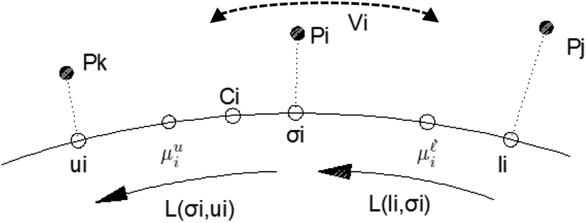
Curvature-weighted deployment. P_i , P_j and P_k represent the positions of the USVs; σ_i , u_i and l_i represent USVs’ projections on the boundary; $μ_{i}^{u}$ and $μ_{i}^{l}$ represent the midpoints between l_i and σ_i ; σ_i and u_i are calculated according to pseudo range D_λ ; V_i represents the Voronoi cell associated with the USV i; Ci represents the Voronoi centre. USV: unmanned surface vehicle.

The objective of the USV distribution is to distribute in such a way that their Voronoi cell has pseudo-length equal to

D_{λ}^{*} = \frac{1}{n} \int_{0}^{1} (λ k^{\frac{1}{3}} (s) + (1 - λ)) r^{'} (s) d s

The curvature-weighted deployment process is shown in Figure 8.

Figure 8.

Curvature-weighted deployment algorithm.

Estimation of the moving boundary points based on Kalman filter and PSO

According to the previous discussion, the motion of oil contamination on the water surface is divided into two stages: diffusion and drift. The oil contamination rapidly spreads after spilling into the water. In the initial spread–inertial expansion stage in the diffusion process, the oil contamination rapidly spreads to form an oval oil contamination. The area slowly expands during the subsequent viscous expansion and surface tension expansion stages. The diameter of the oil contamination remains nearly the same after the expansion process. In other words, in addition to the initial oil spill stage, the movement of oil contamination on the water surface is mostly drift which is mainly affected by the flow and wind fields. Therefore, we mainly consider the effects of the drift process when predicting the motion of oil contamination.

Kalman prediction

The real-time tracking of an entire spatial target is difficult. USVs can only monitor several points in a region at once. Meanwhile, USVs can lose track of monitoring targets due to interference from many environmental factors, such as the influence of changes in flow direction, the diffusion and dispersion of oil films and the obstacles in a region. Therefore, obtaining superior tracking effects, real-time performance and robustness is difficult. The Kalman filter is an algorithm that estimates the linear minimum variance of the state sequence of a dynamic system. It entails minimal computation and realises real-time performance. It can also be used to predict target locations.⁴⁵ Suppose that the interference noise of the objective state and sensors is Gaussian noise. The position of the boundary points of the oil contamination is predicted by the Kalman filter. Furthermore, USVs may lose the monitoring objective given the dispersion and fragmentation of the oil contamination caused by wind, waves or turbulence. This study adopts the PSO algorithm to search the boundary of the objective region. The movement position of the objective point is predicted according to the state equation. The boundary point of the oil contamination is then searched using the PSO algorithm in a local region extended from the predicted objective point. The optimal search result is used as the observation value of the Kalman filter to correct the prediction of the objective point and obtain the optimal estimation value.

Problem statement: The estimated parameters are contained in the state vector X_t , where t is the time stamp. The state vector is a description of the objective, such as position or velocity, which represents the degree of spatial expansion.

Dynamic nature: The estimated state vector is based on the Markoff model: $P (X_{t} |X_{t - 1})$ .

Measurement: A set of measurements could be obtained at each time step: $Z_{t} = {\{Z_{1}, \dots Z_{n}\}}_{t}$ . These measurements are derived from random searches near the objective points. Assume that the measured results are independent of one another and are only related to state X_t of moment t.

For the points on the oil contamination boundary, if the velocity at point k is u^k , then the predicted position could be calculated by

X_{t}^{k} = X_{t - 1}^{k} + \int_{t_{0}}^{t_{0} + Δ τ} u^{k} d t

where $Δ τ$ is the time step. The system is a linear system.

For simplicity, some assumptions regarding the velocity of oil contamination are presented.

The speed of the entire contamination is similar to its centroid point.

Only the influential factors of water flow and wind field are considered. The influence of tide, earth rotating flow and other factors are ignored.

Therefore, the drift velocity of point k is as follows: $u_{}^{k} = u_{wind}^{k} + u_{flow}^{k}$ .

The velocity of the wind used in the calculation usually takes a value of 0.0035 times the wind speed for a 10 m height above the water surface, m/s. The wind speed is monitored by the environmental monitoring station, and the water flow speed is measured by the Doppler velocity sensor carried by each USV.

According to the Kalman filter equations

X_{t} = A X_{t - 1} + W_{t - 1}

Y_{t} = C X_{t} + V_{t}

where $X_{t}, X_{t - 1}$ is the state vector at time t and t − 1, and Y_t is the observational vectors at time t. $X_{t} = |\begin{matrix} x_{t} \\ y_{t} \\ x_{t}^{'} \\ y_{t}^{'} \end{matrix}|$ and $Y_{t} = |\begin{matrix} x_{o t} \\ y_{o t} \end{matrix}|$ , where the elements in X_t represent the x and y coordinates of the boundary points and the corresponding velocity. The elements of $Y_{t}$ are the observed values of the corresponding target point.

$x_{t}^{'}$ and $y_{t}^{'}$ are the drift velocity elements in the horizontal and vertical directions, respectively, where $[\begin{matrix} x_{t}^{'} \\ y_{t}^{'} \end{matrix}] = |\begin{matrix} (x_{t} - x_{t - 1}) / Δ t \\ (y_{t} - y_{t - 1}) / Δ t \end{matrix}|$ .

According to the motion of the points on the oil film, A and C can be represented as follows

A = [\begin{matrix} 1 & 0 & Δ τ & 0 \\ 0 & 1 & 0 & Δ τ \\ 0 & 0 & 1 & 0 \\ 0 & 0 & 0 & 1 \end{matrix}]

C = [\begin{matrix} 1 & 0 & 0 & 0 \\ 0 & 1 & 0 & 0 \end{matrix}]

W is the system noise which has a Gaussian distribution. Its mean value is zero, and its covariance matrix is $Q = 0.01 \times U$ , where U is the unit matrix of $4 \times 4$ .

V represents the observation noise which has a Gaussian distribution. Its mean value is zero, and its covariance matrix is R.

The initial state at $t = 0$ is $X_{0} = {[x_{0}, y_{0}, x_{0}^{'}, y_{0}^{'}]}^{T}$ , where $x_{0} and y_{0}$ are the coordinates of the distribution point on the boundary. $x_{0}^{'} and y_{0}^{'}$ are the velocities of drift oil contamination, ${[x_{0}^{'}, y_{0}^{'}]}^{T} = |\begin{matrix} u_{t}^{k} \cdot cos θ \\ u_{t}^{k} \cdot sin θ \end{matrix}|$ . θ is the angle between the flow and horizontal directions.

Objective boundary point detection based on PSO

After the position of the objective boundary point is predicted by the Kalman filter, the real boundary point is searched by the nearby USV. The position of the searched point is considered an observation value to perform the next step of prediction. Given that the USV cannot directly detect the boundary point, an effective measure is to allow the USV to cross the boundary curve. The midpoint between two adjacent sampling points containing the step change of pollution concentration is considered to be the contaminated boundary point. Jaward et al.⁴¹ use a searching method along the normal direction of the boundary curve to detect boundary points. This method is simple and effective when the boundary curve is continuous and complete. However, the boundary of the oil contamination may occasionally be discrete and discontinued in a certain drift stage, and the USV may lose the target. 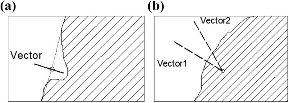For example, when the USV moves to the location of the predicted boundary point, two possible sampling values are available: $S_{k} = 0$ and $S_{k} = 1$ (as shown in equation (2)). As shown in Figure 9(a), $S_{k} = 0$ means that the predicted location of the point is outside the oil contamination region. At this time, the searching method along the normal direction loses the objective result from the discrete oil film boundary. $S_{k} = 1$ means that the predicted point is located inside the oil film region. Meanwhile, boundary points can be detected along the normal vector. However, the deviation of the prediction for the boundary curve may cause the normal vector to deviate from the correct direction, thereby generating a large deviation, as displayed in vectors 1 and 2 in Figure 9(b).

Figure 9.

Possible predicted position. (a) S_k = 0 and (b) S_k = 1.

A rectangular region with width W and height H is expanded to effectively detect the objective boundary points. The centre point $(x_{0}, y_{0})$ of the rectangular region is predicted by the Kalman filter. The nearest boundary point from the prediction point is searched in this region. The PSO algorithm is used in this study to quickly find the global optimum point in the region. PSO is an evolutionary calculation method based on swarm intelligence. Compared with the general evolutionary algorithm, PSO can be easily realised. This algorithm needs few adjusted parameters and is usually used in spatial optimisation.^46,47

The basic PSO algorithm is expressed in the following. Assume that the search space of N dimensions comprises populations with N particles, where the position of each particle can be expressed as a vector of X_i = (x_i ₁, x_i ₂…x_in )^T. According to the objective function, the fitness value corresponding to each particle’s position X can be calculated. The velocity of the ith particle is expressed as V_i = (v_i ₁, v_i ₂…v_in )^T, and its individual extreme values denote the optimum historical position of the particle, which is expressed as P_i = (P_i ₁, P_i ₂…P_in ). The extreme value of the population is the optimum historical position of particle populations, which are expressed as P_g = (P_g ₁, P_g ₂…P_gn ). In the qth iteration, the updating formula of particle velocity and position is as follows

v_{i}^{q + 1} = w v_{i}^{q} + c_{1} r_{1} (P_{i}^{q} - X_{i}^{q}) + c_{2} r_{2} (P_{g}^{q} - X_{i}^{q})

X_{i}^{q + 1} = X_{i}^{q} + v_{i}^{q + 1}

where w is the inertia weight which represents the degree of inertial motion of a particle in accordance with its own velocity. It is linearly reduced with the number of iterations

w = w_{max} - t \cdot \frac{w_{max} - w_{min}}{t_{max}}

w_{max} = 0.9

w_{min} = 0.4

c ₁ and c ₂ are learning factors which represent the experience learned from the particle and the particle group, respectively. The values of c ₁ and c ₂ are usually 2. r ₁ and r ₂ are random numbers between 0 and 1. t is the current step of iterations, and t _max is the max step of iterations.

Algorithm implementation

The information collection process of a USV is as follows: moving forward → stopping and collecting data → moving to the next destination. According to the response time of the sensor, the time needed for data collection is approximately 5 s in each step. The value of the collected water quality data is recorded as S_x . USVs can obtain their own coordinates $(x_{k}, y_{k})$ during operation. The distance d_k from the initial point $(x_{0}, y_{0})$ could be calculated by

d_{k} = \sqrt{{(x_{k} - x_{0})}^{2} + {(y_{k} - y_{0})}^{2}}

The detection of the boundary point is determined by the presence of the maximum difference of the sample values $abs (S_{x (k)} - S_{x (k - 1)})$ between two adjacent sampling points. The maximum difference value is 1 or 0 due to the binary nature of the sensed data. Considering the possible presence of more than one boundary point in a region, we take the boundary point closest to the initial point $(x_{0}, y_{0})$ as the detected boundary point.

Therefore, the distance parameters are considered in the fitness function.

Equation (14) is the fitness function

\frac{abs (S_{x (k)} - S_{x (k - 1)})}{d_{k}}

The flow of the boundary point search based on the PSO algorithm is as follows.

Step 1: Set the search area according to the initial point $(x_{0}, y_{0})$ .

Step 2: The USV randomly travels to several positions in the area. These positions are considered as several particles of the PSO. Particles are in 2D spaces. The position of a particle is $(x_{k}, y_{k})$ . The speed range is 0.2–0.5 m. Particle velocity could be regarded as the range of movement of a particle in a step.

Step 3: Update the velocity of each dimension of a particle by equation (11) and its boundary constraint (replace the value exceeding [ $- v_{max}$ , $v_{max}$ ] with the boundary value). Update the dimension positions of the particle according to equation (12). The $v_{i}^{q + 1}$ in equation (11) is a vector $[v_{x i}^{q + 1}, v_{y i}^{q + 1}]$ , and the $X_{i}^{q + 1}$ in equation (12) is vector $[v_{x i}^{q + 1}, v_{y i}^{q + 1}]$ , indicating the velocity and position coordinates of the particles in the x and y directions, respectively.

Step 4: Calculate the fitness function for each particle according to equation (13), and update $P_{i}^{q}$ and $P_{g}^{q}$ .

Step 5: Repeat step 3 for iteration until the maximum number of iterations is reached or a convergence condition is met.

The best boundary point obtained by the PSO is taken as the Kalman filter observation and as the object of the next step.

A large number of USVs lead to a high tracking accuracy. However, in the case of a limited number of USVs, the approach must be improved to obtain tracking points further. According to the USV distribution obtained by the curvature weight distribution logic, the USV distributes some interpolation points in its Voronoi cell. As shown in Figure 10(a), four USVs are uniformly distributed on the boundary curve (red dots in Figure 10), and the interpolation points are evenly distributed (green dots in Figure 10). Consequently, the USV detects the position of each point. Each USV can only detect the position of one point in each moment, and the PSO–Kalman method can be used to estimate the position of the points (red dots in Figure 10(a)). 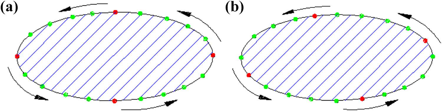The remaining points are estimated according to equation (8), with u^k value of $(X_{t} - X_{t - 1}) / Δ t$ . Subsequently, the agent moves counterclockwise to the neighbouring point and estimates the position with the PSO–Kalman method (red dots in Figure 10(b)). This method is named CPK by us.

Figure 10.

Circle detection of the motion contour in (a) time t and (b) time t + 1.

Overall flow of the tracking method for drift oil spill contamination

Given that the monitored water area usually has a wide range and contamination with flow presents dynamic features, the overall tracking work should preferably be performed by cooperative multi-USV. The area coverage can be obtained faster by multi-USV than by a single USV. The pollution pheromone could also be quickly found. When performing the tracking task, if many USVs are available in the system, then the selection and coordination of multi-USV are necessary. The first USV to find the contamination becomes a temporary leader. Other USVs are called to form a team together. At this moment, the lead USV is similar to a tenderee, and others are bidders. The tenderee sends out collaborative applications to other USVs. The relevant information regarding the mission is also sent. When the bidder receives the task information of the tenderer, it will bid according to the work requirements and its own condition. The following factors are considered: (1) bidders’ current task, (2) path length, (3) time needed on the task and (4) task performance of the bidder. The bidders evaluate the task and provide feedback to the tenderee. The tenderee compares and sequences the feedback information from different bidders. The most suitable bidders are selected as winning bidders. The winning bidder must be a USV that is most suitable as a cooperative partner in terms of the comprehensive consideration of time, distance, importance and proficiency. The details of partner selection can be found in the literature.⁴² After the team is formed, the USV leader assigns the paths of the other members to detect the contour of the contaminated area, as shown in Figure 6(a). After the contour of the contamination is initially detected, each member is assigned and distributed on the oil film boundary of their own Voronoi cell (Figure 7). Multi-USV moves along with the contamination on the basis of the PSO–Kalman method. Each USV has its own path and demonstrates cooperation to complete the mission (Figure 10).

The overall flow of the tracking method for drift oil spill pollution is shown in Figure 11 and is summarised as follows.

Multi-USV moves in formation to search for information about the pollution plume in the target region. The zigzag working method is adapted to cover the target area (detailed in ‘Pollution information searching behaviour’ section).

When a USV detects the pollution plume information, it uses the clover search method to confirm whether the pollution is a sporadic plume or a wide range of oil film (detailed in ‘Detection and confirmation of pollution information’ section). If the pollution is determined as sporadic oil pollution, then the zigzag search is performed. If the pollution is a wide range of oil film, then the USV calls for other members to perform the task.

After the team is formed, the implementation of UUV-gas edge detection is conducted (detailed in ‘Contour detection of oil film contamination’ section).

After exploring the entire boundary of the oil film, multiple USVs are distributed along the boundary of the oil film according to the curvature weight distribution logic (detailed in ‘Obtaining the deployment nodes along the contour’ section).

The CPK method is then used to trace and estimate the location of the boundary points (detailed in ‘Estimation of the moving boundary points based on Kalman filter and PSO’ section which is the main contribution of this work). The map of the boundary curve is drawn in each time step.

The tracking work is performed until the end message is received.

Figure 11.

Overall flow of the proposed method.

Case study

Simulations of the cases in four scenes

The following simulation examples are presented to illustrate the operation of the proposed approach and its implementation.

A dynamic contour is simulated in MATLAB. The max simulation space is set to 200 × 100 m². Moving oil contamination is simulated as a monitoring target. The target moves on a 2D plane according to the discrete hour order (constant velocity) model with a uniform time interval between measurement frames: $X_{t} = A X_{t - 1} + W_{t - 1}$ , where $X = {(x, \dot{y, x, \dot{y}})}^{T}$ , $W = {(w_{X}, w_{Y})}^{T}$ and $A = [\begin{matrix} 1 & 0 & Δ τ & 0 \\ 0 & 1 & 0 & Δ τ \\ 0 & 0 & 1 & 0 \\ 0 & 0 & 0 & 1 \end{matrix}]$ . W_t is modelled as zero mean while Gaussian noise with covariance $E [W_{k} W_{k}^{T}] = q I_{2}$ , where I ₂ is the 2 × 2 identity matrix. For this case, the variance of the acceleration noise is q = 0.1. Each frame of measurements comprises a set of XY Cartesian pairs. Measurements from the target are independent, zero mean Gaussian perturbation with R = diag $\{1, 0.1\}$ . Some scenes are simulated to validate the proposed approach.

Scene 1: Contamination detection

The simulation of contamination detection for scene 1 is shown in Figure 12. Four agents are simulated to detect contamination with an average speed of 0.3 m/s. The measurement radius of the sensor is set to 1 m. Agents perform the zigzagging behaviour to capture the plume of the contamination. Once the agent detects and confirms the oil plume, other agents are summoned to trace the contour of the contamination together. The points in Figure 12 are the trail of agents, and the ellipse line is the contour of the contamination. USV1 detects the oil contamination plume and calls three other USVs to help with detection. Four USVs cooperate together to successfully detect the contour of the oil film (Figure 12).

Figure 12.

Simulation of contamination detection. I: trajectory of USV1, II: trajectory of USV2, III: trajectory of USV3 and IV: trajectory of USV4. USV: unmanned surface vehicle.

Scene 2: Tracking of the moving contamination in the drift stage

Figure 13 shows the trajectory of contamination which is supposed to have a constant velocity of 0.035 m/s. Suppose the contamination is in a non-diffusion stage with a stable contour. As shown in Figure 13, the observed trajectory is continuously vibrating due to the observation noise. The black curve is the simulated real contour of the oil film, which is estimated to have a stable boundary and is moving at a constant speed. The blue points in the figure are the points observed by the USVs. The red curve is the contour of the oil film predicted by the Kalman filter. The time step of the monitoring is 10 min/step. The curves in Figure 13 are the states in the first seven steps. As shown in the simulated result in Figure 13, a good tracking effect exists in the predicted curve compared with the real trajectory.

Figure 13.

Tracking simulation of the moving contamination in the drift stage.

As shown in Figure 14, the green points are the mean errors before filtering in each step, and the red points are the mean errors after filtering. This finding shows that the mean error is effectively reduced by our proposed approach.

Figure 14.

Mean errors before and after filtering in scene 2.

Scene 3: Tracking of the moving contamination in the diffusion stage

Figure 15 shows a scene in which the contamination is in a diffusion stage with an isotropic diffusion speed of 0.004 m/s. The filter can maintain tracking and demonstrate satisfactory performance.

Figure 15.

Simulation of tracking of the moving contamination in the diffusion stage.

Scene 4: Tracking of the moving contamination in the drift stage with changing flow direction

Figure 16 shows a scene in which the contamination is in a diffusion stage with changing flow direction. The direction of the water flow changes in four stages. Despite the increase in tracking errors in steps 4 and 5, the method still shows a good adaptation to maintain tracking in changed environments.

Figure 16.

MATLAB simulation of tracking of the moving contamination in the drift stage with changing flow direction.

Comparison tests

A few comparison tests are performed to verify the advantage of the proposed method. The tracking simulation is conducted by the methods with and without CPK. The simulation, beginning with the multi-USV, completes the initial contour detection and prepares to track the moving contamination. In the method without CPK, the USV only employs the UUV-gas algorithm when tracking the contamination. The tracing process is same in steps (1) to (4) but different in step (5) as shown in ‘Overall flow of the tracking method for drift oil spill contamination’ section. When the USVs move along the edge of the contamination, they only turn clockwise and counterclockwise when they are inside and outside the perimeter, respectively.

The contour points detected by USVs are connected to form the contour line. The area (A_t ) enclosed by the contour line is computed and compared with the real area (A_r ) of the contamination. The relative error is computed as follows

σ = \frac{|A_{t} - A_{r}|}{A_{r}}

The test is lasted 70 min each time. The average relative error of each monitoring step is recorded.

The first test is run several times with different moving speeds of contamination in scene 2. The test is repeated run four times in each moving speed, and the average relative error is recorded. The result is shown in Figure 17.

Figure 17.

Comparison of average relative errors with varied speeds in scene 2.

The tracking effect is influenced by the moving speed of the contamination. The average relative error increases with a rise in the contamination moving speed. The average relative error of the method without CPK is higher than that of the method with CPK. At the speed of 0.1 m/s, the average relative error of the method without CPK reaches 32.88%, which could be nearly regarded as tracking failure. However, the average relative error of the method with CPK slowly increases. This finding means that the contour of contamination can be successfully tracked and that the detection error can be effectively reduced using the proposed method.

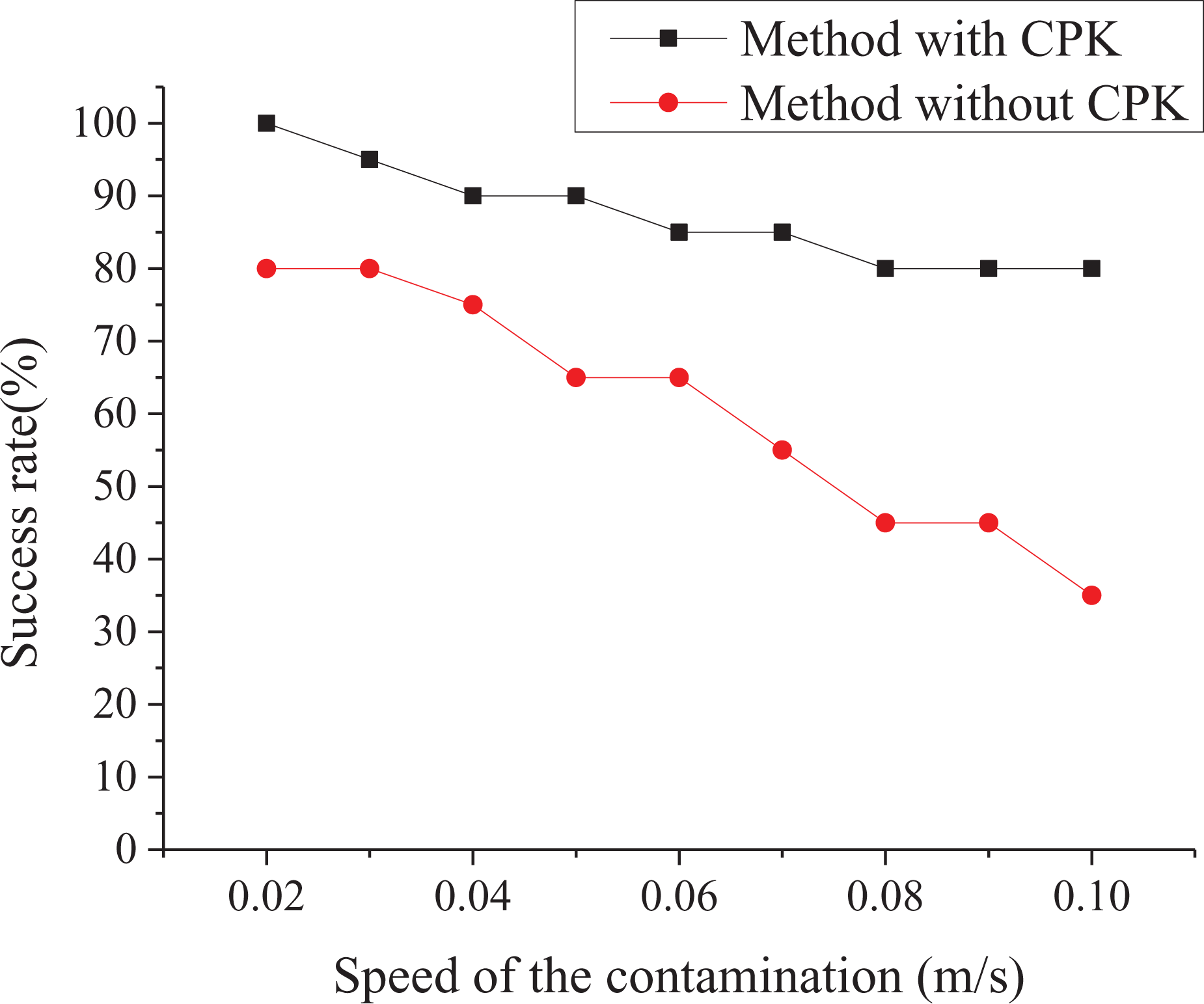
The second test is run four times with different contamination diffusion speeds in scene 3. The success rate of the tracking is recorded in this test. The relative error of more than 30% is regarded as tracking failure, and the result is shown in Figure 18. The success rate decreases with an increase in the contamination diffusion speed. The success rate of the method CPK is higher than that of the method without CPK. This finding means that the proposed method is more effective than the existing method for tracking moving contamination in the diffusion stage.

Figure 18.

Comparison of success rates with varied speeds in scene 3.

The third test is run four times with changing flow direction in the diffusion stage, similar to that in scene 4. The moving speed of the contamination is increased, and the result is shown in Figure 19. The success rate decreases with an increase in the contamination diffusion speed. The success rate of the method CPK is higher than that of the method without CPK. The proposed method is more effective than the existing method for tracking moving contamination in water environments with varied flow directions.

Figure 19.

Comparison of success rates with varied speeds in scene 4.

The last test is run with contamination moving speeds of 0.04 m/s and diffusion speeds of 0.006 m/s. The flow direction is unchanged. The relative errors are recorded in each record step. The interval between each record step is 10 min. From Figure 20, it can be seen that the relative error is increased with time. The relative error of method with CPK is increasing slowly while the relative error of method without CPK is increasing fast. The relative error of method with CPK is accumulated more and more over time. Therefore, the method with CPK shown more better performance than the method without CPK.

Figure 20.

Comparison of relative errors in each record step of one test.

Discussion

The performance of the proposed method is conveniently assessed via simulations. The tracking effect is excellent under the condition in which the oil pollution feature is known and the flow velocity and direction could be easily detected. In cases of tracking moving contamination in the drift stage, diffusion stage and water environments with changing flow directions, the proposed method exhibits good performance and successfully tracks the target (Figures 12 to 16). The mean error is effectively reduced by the proposed approach.

Another major asset of the employed tracking method is its robustness with respect to the water environment. The robustness of the method with respect to the speed and diffusion of contamination with flow is tested, as shown in Figures 17 and 18, respectively. The robustness of the method with respect to the changing flow direction is also tested, as shown in Figure 19. Figure 20 shows that the relative error of method without CPK is accumulated more and more over time. Herein, we quantitatively demonstrate this robustness by testing the method in simulations with well-detected flow parameters of the environment. Both cases show similar characteristics. Although the environment exhibits minimal influence, the method remains effective and demonstrates a high success rate. On the contrary, the method without CPK shows poor robustness and a low success rate under rapid flow and diffusion conditions, especially in varied flow.

The proposed method is used to control the designed real multi-USV system. The multi-USV system is used to monitor the water quality of an artificial lake located in the Shanghai University of Engineering Science. This method is currently in the testing phase. Nevertheless, the test condition of the water environment is simple. The effectiveness and robustness of the method when executed in a complex water environment should be verified in the future. For example, the performance in fast and time-variant flow-field environments should be improved. The studies by Li et al.⁴³, Kwok and Martínez⁴⁴ and Zhang Weiwei et al.⁴⁸ could serve as a reference to resolve the issues that may be encountered in the future.

Conclusion

This article presents an adaptive agent tracking approach for oil pollution. While considering the dynamic characteristics of water contamination, agents are used in water environment monitoring. The approach is based on the integration of a tracking framework. The zigzag method is used to capture the plume of the contamination. After the oil plume is detected, the extensiveness of the oil pollution is identified by the cloverleaf trajectory method. The UUV-gas method is then used to detect the contour of the pollution area. Multi-USV is deployed on the contour according to the CDA. A CPK method is proposed to track and estimate the moving position of the pollution contour. Some scenes are simulated in MATLAB to validate the proposed approach. Four USVs are also simulated to track the oil film in different scenes. Our case study shows that the proposed method can maintain tracking and achieve a satisfactory performance in cases of moving contamination in different stages.

In the future, additional experiments must be conducted in a large scale and complex water environment to test the suitability and robustness of the approach.

Footnotes

Declaration of conflicting interests

The author(s) declared no potential conflicts of interest with respect to the research, authorship, and/or publication of this article.

Funding

The author(s) disclosed receipt of the following financial support for the research, authorship, and/or publication of this article: This paper was supported by the Natural Science Fund of China (NSFC) under Grant Nos. 51575186, Shanghai Science and Technology Action Plan under Grant No. 18DZ1204000, 18510745500, 18510750100, 18510730600, Shanghai Aerospace Science and Technology Innovation Fund (SAST) under Grant No. 2019–080, 2019–116.

ORCID iD

Xiaoci Huang

References

Petriu

Whalen

Abielmona

, et al. Robotic sensor agents: a new generation of intelligent agents for complex environment monitoring. IEEE Instru Meas Mag 2004; 7(3): 46–51.

Abielmona

Petriu

Harb

, et al. Mission-driven robotic intelligent sensor agents for territorial security. IEEE Comput Intell Mag 2011; 6(1): 55–67.

Gâteau

Ouedraogo

Feltus

, et al. Adopting trust and assurance as indicators for the reassignment of responsibilities in multi-agent systems. Knowl Eng Rev 2015; 30(2): 187–200.

Ball

Qela

Wesolkowski

. A review of the use of computational intelligence in the design of military surveillance networks. In: Abielmona

Falcon

Zincir-Heywood

Abbass

(eds), Recent advances in computational intelligence in defense and security. Studies in computational intelligence, Vol. 621. Cham: Springer, 2016, pp. 663–693.

Huang

Cao

Gao

, et al. Numerical simulation of oil spill drift-diffusion in the Bohai Sea. Mar Sci 2014; 11: 100–107.

Chen

, et al. Numerical simulation of oil spill in the Gulf of Mexico based on the GNOME and ADIOS. Mar Environ Res 2013; 32(4): 599–604.

Huan

Shao

Cheng

, et al. Research on numerical prediction technology of oil spill spreading, drift and diffusion. Bull Mar Sci 2017; 36(4): 379–384.

Cheng

W-P

Liao

Chen

, et al. Reconstruct of pollution cloudy based on backward density probability function diffusion equation. J Sichuan Univ: Eng Sci Ed 2012; 44(4): 35–41.

Gilholm

Salmond

. Spatial distribution model for tracking extended objects. In: IEE Proceedings – Radar, Sonar and Navigation, Vol. 152(5), 17 October 2005, pp. 364–371. IET.

10.

Majid

MHA

Arshad

. Design of an autonomous surface vehicle (ASV) for swarming application. In: Autonomous underwater vehicles, Tokyo, Japan, 6–9 November 2016, pp. 230–235. Washington: IEEE.

11.

Vitor

AMJ

Granada

Maidana

, et al. A survey on unmanned surface vehicles for disaster robotics main challenges and directions. Sensors 2019; 19(702): 1–44.

12.

Brown

Tuggle

Macmahan

, et al. The use of autonomous vehicles for spatially measuring mean velocity profiles in rivers and estuaries. Intel Serv Robot 2011; 4(4): 233–244.

13.

Furfaro

Dusek

Ellenrieder

KDV

. Design, construction, and initial testing of an autonomous surface vehicle for riverine and coastal reconnaissance. In: Oceans, Biloxi, MS, USA, 26–29 October 2009, pp. 1–6. New York: IEEE.

14.

Bhattacharya

Heidarsson

Sukhatme

, et al. Cooperative control of autonomous surface vehicles for oil skimming and cleanup. In: International conference on robotics and automation, Shanghai, China, 9–13 May 2011, pp. 2374–2379. New York: IEEE.

15.

Alami

Fleury

Herrb

, et al. Multi-robot cooperation in the MARTHA project. Robot Auto Mag IEEE 1998; 5(1): 36–47.

16.

Budinska

Havlik

. Task allocation within a heterogeneous multi-robot system. In: Cybernetics & informatics, Levoca, Slovaki, 2–5 February 2016, pp. 1–5. New York: IEEE.

17.

Yan

Jouandeau

Ali

. A survey and analysis of multi-robot coordination. Int J Adv Robot Sys 2013; 10(1): 1.

18.

Amanda

Bahr

Martinoli

. Low-cost collaborative localization for large-scale multi-robot systems. In: Proceedings of ICRA’12, Saint Paul, MN, USA, 14–18 May 2012, pp. 4236–4241. New York: IEEE.

19.

Khalil

Beveridge

Sthilaire

. Assessment of the Lake Winnipeg water quality monitoring network. Research Report # R-1197. Québec, Canada: INRS-ETE, 2010.

20.

Kemp

Bertozzi

Marthaler

. Multi-UUV perimeter surveillance. In: 2004 IEEE/OES autonomous underwater vehicles, Sebasco, ME, USA, USA, 17–18 June 2004, pp. 102–107. New York: IEEE.

21.

Trincavelli

Reggente

Coradeschi

, et al. Towards environmental monitoring with mobile robots. In: International conference on intelligent robots and systems, Nice, France, 22–26 September 2008, pp. 2210–2215. New York: IEEE.

22.

Kato

(Ed.). Applications to marine disaster prevention: Spilled oil and gas tracking buoy system. 1st edn. Tokyo, Japan: Springer, 2017, p. 201.

23.

Senga

Kato

Ito

, et al. Spilled oil tracking autonomous buoy system. Adv Robotics 2009; 23(9): 1103–1129.

24.

Fahad

Saul

Guo

, et al. Robotic simulation of dynamic plume tracking by unmanned surface vessels. In 2015 IEEE International Conference on Robotics and Automation (ICRA), 2015, pp. 2654–2659. IEEE.

25.

Sun

Yao

Zhang

. A novel supervised level set method for non-rigid object tracking. In: IEEE conference on computer vision and pattern recognition, Colorado Springs, CO, USA, 20–25 June 2011, pp. 3393–3400. New York: IEEE.

26.

Zhang

Pece

AEC

. Visual contour tracking based on particle filters. Image Vis Comput 2003; 21(1): 111–123.

27.

Sun

Yao

Zhang

, et al. Non-rigid object contour tracking via a novel supervised level set model. IEEE Trans Image Process 2015; 24(11): 3386–3899.

28.

Kanagamalliga

Vasuki

. Contour-based object tracking in video scenes through optical flow and gabor features. Int J Light Elect Opt 2017; 157: 787–797.

29.

J-H

. Tracking of moving object based on genetic algorithm and Kalman filter. J Comput Appl 2007; 27(4): 916–918.

30.

Farrell

Pang

, et al. Moth-inspired chemical plume tracing on an autonomous underwater vehicle. IEEE Trans Robot 2006; 22(2): 292–307.

31.

Hou-jin

Zhang

Wang

, et al. Classifying and estimating the movement patterns, oil spill volumes and pollution levels of oil spills on the sea. Environ Dev Sustain 1989; (7): 12–14.

32.

Fay

. The spread of oil slicks on a calm sea. In: Hoult

(ed.), Oil on the sea. Ocean Technology. Boston, MA: Springer, 1969, pp. 53–63.

33.

Chen

X-Y

Zhu

Zhang

. Analysing the oil spill extended rule of Bohai estuary wharf. Wat Sci Eng 2009; 2(5): 4–7.

34.

Russell

Bab-Hadiashar

Shepherd

, et al. A comparison of reactive robot chemotaxis algorithms. Robot Auto Sys 2003; 45(2): 83–97.

35.

Hayes

Martinoli

Goodman

. Distributed odor source localization. IEEE Sens J 2002; 2(3): 260–271.

36.

Yao

Finding efficient robot path for the complete coverage of a known space. In: International conference on intelligent robots and systems, Beijing, China, 9–15 October 2006, pp. 3369–3374. New York: IEEE.

37.

Acar

Choset

Rizzi

, et al. Morse decompositions for coverage tasks. Int J Robot Res 2002; 21(4): 331–344.

38.

Min

Yin

. A decentralized approach for cooperative sweeping by multiple mobile robots. In: Proceedings of international symposium on semiconductor manufacturing, Victoria, BC, Canada, 17 October 1998, pp. 323–340. New York: IEEE.

39.

Kurabayashi

. Cooperative sweeping by multiple mobile robots with relocating portable obstacles. In: IEEE/RSJ international conference on intelligent robots and systems ’96 (ed Yoshida

), Vol. 3. Osaka, Japan, 8 November 1996, pp. 1472–1477. New York: IEEE.

40.

Susca

Martinez

Bullo

. Monitoring environmental boundaries with a robotic sensor network. In: American control conference, Minneapolis, MN, USA, 14–16 June 2006, p. 6. New York: IEEE.

41.

Jaward

Bull

Canagarajah

. Contour tracking of contaminant clouds with sequential Monte Carlo methods. In: IEEE international conference on acoustics, speech and signal processing, Las Vegas, NV, USA, 31 March–4 April 2008, pp. 1469–1472. New York: IEEE.

42.

Shaoxuan

. Multi-robot cooperation and coordination based on ant colony algorithm. J Shenyang Ligong Univ 2011; 30(5): 45–49.

43.

J-G

Meng

, et al. Tracing odor plume by robot in time-variant flow-field environments. Acta Automatica Sinica 2009; 35(10): 1327–1333.

44.

Kwok

Martínez

. Coverage maximization with autonomous agents in fast flow environments. J Optimiz Theory App 2012; 155(3): 986–1007.

45.

Chang

F-L

Liu

Wang

. Target tracking algorithm based on meanshift and Kalman filter. Comput Eng Appl 2007; 43(12): 50–52.

46.

Doctor

Venayagamoorthy

Gudise

. Optimal PSO for collective robotic search applications. Evol Comput 2004; 2: 1390–1395.

47.

Khatami

Mirghasemi

Khosravi

. A new PSO-based approach to fire flame detection using K-Medoids clustering. Expert Syst Appl Int J 2017; 68(C): 69–80.

48.

Zhang

Zheng

. Part-Aware region proposal for vehicle detection in high occlusion environment. IEEE Access 2019; 99(7): 100383–100393.

Adaptive agent tracking approach for oil contamination in water environments

Abstract

Keywords

Introduction

Related work

References review

Contributions

Problem statement

Dynamic feature of oil contamination

Design of the multi-USV system

Physical structure of single USV

Topological logic for cooperative decision-making of multiple USVs-remote centre

Purpose of this study

Materials and methods

Pollution information searching behaviour

Detection and confirmation of pollution information

Contour detection of oil film contamination

Obtaining the deployment nodes along the contour

Estimation of the moving boundary points based on Kalman filter and PSO

Kalman prediction

Objective boundary point detection based on PSO

Algorithm implementation

Overall flow of the tracking method for drift oil spill contamination

Case study

Simulations of the cases in four scenes

Scene 1: Contamination detection

Scene 2: Tracking of the moving contamination in the drift stage

Scene 3: Tracking of the moving contamination in the diffusion stage

Scene 4: Tracking of the moving contamination in the drift stage with changing flow direction

Comparison tests

Discussion

Conclusion

Footnotes

Declaration of conflicting interests

Funding

ORCID iD

References