Locomotion generation for a mobile manipulator by global minimization of the weighted generalized momentum

Abstract

This article presents a method for generating the locomotion of a mobile manipulator that globally minimizes the weighted generalized momentum. The method utilizes the calculus of variation setting to address the problem for which the optimal trajectory may be computed by solving the initial value problem of the system of ordinary differential equations rather than the two-point boundary value problem. Online optimal trajectory may then be input to a suitable tracking controller for controlling the robot in real time. Effectively, the robot closed-loop dynamics is shaped to the optimal system such that the locomotion minimizes the difference of the weighted generalized momentum and the assigned potential energy under the constraints imposed on by the tracking task, joint angle, and actuator torque limits. Desired locomotion behaviors may be achieved by properly adjusting the weighting, spring, and damping matrices. Exploiting the induced dynamical force from the cooperative motion of the constituent linkages through the momentum minimization basis, the robot is able to outperform conventional locomotion pattern actuated by the platform solely.

Introduction

A mobile manipulator, hereafter called a robot for short, generally consists of the mobile platform and the mounted manipulator. ^1,2 Together, the number of degrees of freedom (DOFs) the robot owned is usually more than required to execute the tasks, that is, the robot is redundant. Hence, it is capable of performing manipulation tasks with high dexterity at different places. Redundancy may also be useful to locomotion, which is the topic of this article. Typically, the mobile base is locomoted to the desired place and then the manipulator can perform tasks at that location. It is observed that during the relocation, the manipulator does not perform any specific task and commonly will be kept at rest relative to the base.

This motion strategy is simple since it put away with the motion planning on those redundant coordinates. Control is also simplified to the regulation control problem. However, it is evident that the animal limbs move during locomotion. While walking or running, human arm naturally swings in opposite direction to the leg motion even though it can be kept fixed deliberately. Studies showed that such arm motion reduces the metabolic energy consumed. ^3,4 Such motion can be observed in advanced robot counterparts. For example, the mobile robot “Handle” ⁵ or the humanoid robot “Atlas” ⁶ is capable of performing energetically impressive locomotion using the whole body motion. This would not be possible using the leg movement solely.

When someone on a boat fires a gun, the boat moves in the opposite direction to the bullet. This phenomenon is explainable by the conservation of momentum, that is, momentum of the bullet is canceled by that of the boat. Hence, motion of the boat is induced by that of the bullet. Such induced motion can be seen in human and robot locomotion caused by complex interplay of the coupled forces. It may be understood as the system strives to conserve the momentum in a manner that movement of all linkages helps driving the body as a whole. Note that when the system is initially at rest, its momentum is zero. Hence, attempting to conserve the momentum implies minimizing its magnitude subject to the motion constraint. With this strategy, the energy spent in the locomotion can be minimized. Moreover, torques that execute the motion will come from all joints rather than their subset at the platform. This inspires us to design the locomotion of redundant mobile manipulators based on the momentum minimization criteria.

Appropriate trajectory generation for the redundant DOFs robot is necessary in order to fully exploit its capability. This may be achieved by computing the robot joint trajectory from the specified task trajectory via pseudoinverse of the task Jacobian matrix and its null space projection ⁷ to locally minimize the joint velocity norm and satisfying additional criteria. Chang ⁸ and Sciavicco and Siciliano ⁹ introduced an extra task through the corresponding Jacobian matrix that may be augmented to the original task. Joint trajectory is now readily determined by the inverse of the augmented Jacobian matrix. Alternatively, pseudoinverse of the higher priority task Jacobian matrix may be used to compute the joint velocity for higher priority task while lower priority task is implemented through the joint velocity in the respective null space. ¹⁰

If the robot input is the actuator torque rather than the velocity, the trajectory generation problem should be considered at the acceleration level. Suh and Hollerbach ¹¹ provided the joint acceleration that locally minimizes the actuator torque norm while tracking the specified task trajectory. Minimization of some integral quantities over the time, known as global minimization problem, was discussed by Suh and Hollerbach, ¹¹ Shiller, ¹² and Kazerounian and Wang ¹³ for torque, time-energy, and joint velocity norm, respectively. Nakamura and Hanafusa ¹⁴ applied Pontryagin’s maximum principle to minimize the integral of the joint velocity norm. Recently, optimal trajectory generation to achieve a set of specified tasks was performed in real time by solving the quadratic programming local optimization problem. ¹⁵ Model predictive control approach may be applied to extend the local toward global optimization by solving the constrained optimal problem over a finite horizon. ¹⁶

This work proposes the weighted generalized momentum (see the “Momentum minimization” subsection) as optimal criteria in planning the locomotion. In this regard, the coordinating coupled force is utilized to help propel the robot as desired. A method (see subsections “Minimization of new Lagrangian” through “Online determination of the optimal trajectory”) to determine the exact optimal solution subject to the tracking task, joint angle, and actuator torque limits is presented. As a result, robot trajectories for different locomotion behaviors according to the specified weighting may be computed online. Required torque will be contributed by all joints cooperatively rather than from merely those at the platform. In addition, the proposed method can be applied to solve a global optimization problem subject to equality and inequality constraints in general.

The article is organized as follows. The second section describes the dynamics of the mobile manipulator and formulates the optimal locomotion generation problem. Rationale of the momentum minimization criteria is explained. In the third section, the optimal system dynamics is derived and a general procedure to compute the optimal solution online subject to equality and inequality constraints is proposed. It is applied to minimize the weighted momentum cost. Simulation and discussion are presented in the fourth section. Finally, conclusions are given in the fifth section.

Problem formulation

Dynamic equations

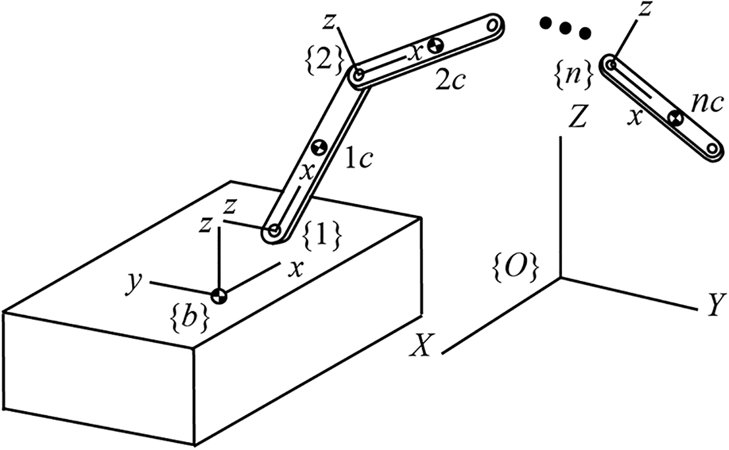
In order to apply the results to general mobile manipulators, detailed realization of the mobile base movement, such as the actuation methods and their arrangement or transmission mechanisms, is not considered. The mobile platform is treated as a rigid body traversing its space. Accordingly, the platform’s postural coordinates and manipulator’s joint angles are chosen as the generalized coordinates. Such simplification generalizes the following development to any mobile robot. Figure 1 displays the robot structure.

Figure 1.

Schematic diagram of a robot comprising the mobile platform and the mounted manipulator.

Let $\left\{O\right\}$ and $\left\{b\right\}$ be the fixed frame and base frame attached to the platform at its center of gravity. Position and orientation of $\left\{b\right\}$ with respect to $\left\{O\right\}$ may be described by the Cartesian coordinates, $p_b=[xyz{]}^{{\rm T}}$ , and unit quaternion, $\epsilon =[{\epsilon }_0{\overline{\epsilon }}^{{\rm T}}{]}^{{\rm T}}=[{\epsilon }_0{\epsilon }_1{\epsilon }_2{\epsilon }_3{]}^{{\rm T}}$ , as $q_b=[p_b^{{\rm T}}{\epsilon }^{{\rm T}}{]}^{{\rm T}}\in {ℝ}^7$ . Configuration of the mounted manipulator may be described by the joint coordinates $q_m=[{\theta }_1,\dots ,{\theta }_n{]}^{{\rm T}}\in {ℝ}^n$ measuring the relative angle or distance of successive linkages. The ith-link is attached with the frame $\left\{i\right\}$ at the joint. $q=[q_b^{{\rm T}}{q}_m^{{\rm T}}{]}^{{\rm T}}$ are the generalized coordinates of the robot.

Velocity of the platform expressed in $\left\{b\right\}$ , ${}^b{V}_b{=[}^b{v}_b^{{\rm T}}{}^b{\omega }_b^{{\rm T}}{]}^{{\rm T}}\in {ℝ}^6$ , is related to ${\dot{q}}_b$ through

${\dot{q}}_b=T(\epsilon ){}^b{V}_b=\left[\begin{array}{cc}{R}_b(\epsilon )& 0\\ 0& E(\epsilon )\end{array}\right]{}^b{V}_b$

1

where

$$\begin{gathered} R_b(\epsilon )=(2{\epsilon }_0^2-1)I+2\overline{\epsilon }{\overline{\epsilon }}^{{\rm T}}+2{\epsilon }_0[\overline{\epsilon }\times ], \\ E(\epsilon )=\frac{1}{2}\left[\begin{array}{c}-{\overline{\epsilon }}^{{\rm T}}\\ {\epsilon }_{0}I+[\overline{\epsilon }\times ]\end{array}\right] \end{gathered}$$

${}^b{V}_b$ is the result of the propulsive velocity ${\eta }_b\in {ℝ}^{6-k}$ caused by full actuation that is consistent with the k-velocity-level platform nonholonomic constraints. They are related through a constant mapping $S\in {ℝ}^{6\times (6-k)}$ ; ${}^b{V}_b=S{\eta }_b$ . Hence, the corresponding constraints can be expressed readily through $A\in {ℝ}^{k\times 6}$ as $A{(}^b{V}_b)=0$ where $AS=0$ . Consequently

${\dot{q}}_b=T(\epsilon )S{\eta }_b=S(\epsilon ){\eta }_b$

2

$AT{(\epsilon )}^{-1}{\dot{q}}_b=0 \text{with} {\epsilon }^{{\rm T}}\dot{\epsilon }=0\Rightarrow A(\epsilon ){\dot{q}}_b=0$

3

describe the platform kinematics. Note that

$T{(\epsilon )}^{-1}=\left[\begin{array}{cc}{R}_b{(\epsilon )}^{{\rm T}}& 0\\ 0& E{(\epsilon )}^{-1}\end{array}\right], E{(\epsilon )}^{-1}=2\left[\begin{array}{cc}-\overline{\epsilon }& {\epsilon }_{0}I-[\overline{\epsilon }\times ]\end{array}\right]$

Assume the manipulator is of serial type and has n-DOFs. Motion of the ith-link is caused by motion of the platform and of link 1 to ith. Velocity of its center of gravity (C.G.) expressed in $\left\{i\right\}$ , ${}^i{V}_i={\left[{}^i{v}_i^{{\rm T}}{ }^i{\omega }_i^{{\rm T}}\right]}^{{\rm T}}$ , is then determined by

${}^i{V}_i={ }^b{\mathcal{R}}_i^{{\rm T}}\left({}^b{J}_b^{i}T{(\epsilon )}^{-1}{\dot{q}}_b+{}^b{J}_m^i{\dot{q}}_m\right)$

4

where ${}^b{\mathcal{R}}_i^{{\rm T}}=\text{diag}\left({}^b{R}_i^{{\rm T}},{\text{}}^b{R}_i^{{\rm T}}\right)$ , ${}^b{R}_i({\theta }_1,\dots ,{\theta }_i)$ is the rotation matrix of $\left\{i\right\}$ with respect to $\left\{b\right\}$ , ${}^b{J}_m^i({\theta }_1,\dots ,{\theta }_i)$ the Jacobian matrix mapping ${\dot{q}}_m$ to ${}^b{V}_i$ , and

${}^b{J}_b^i({\theta }_1,\dots ,{\theta }_i)=\left[\begin{array}{cc}I& -\left[{}^b{p}_{i_c/b}\times \right]\\ 0& I\end{array}\right]$

the Jacobian matrix mapping ${}^b{V}_b$ to ${}^b{V}_i$ , of which ${}^b{p}_{i_c/b}({\theta }_1,\dots ,{\theta }_i)$ is the position vector of the C.G. of ith-link with respect to the origin of $\left\{b\right\}$ . Equation (4) describes the manipulator kinematics.

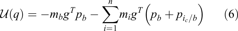
Dynamic equations may be determined using the Lagrange formulation. Lagrangian $\mathcal{L}(q,\dot{q})$ of the robot is defined as $\mathcal{L}={\mathcal{T}}^{*}-\mathcal{U}$ , of which its kinetic co-energy and potential energy are

${\mathcal{T}}^{*}(\epsilon ,q_m,\dot{q})=\frac{1}{2}{}^b{V}_b^{{\rm T}}{\mathcal{M}}_b{}^b{V}_b+{\displaystyle \sum _{i=1}^n}\frac{1}{2}{}^i{V}_i^{{\rm T}}{\mathcal{M}}_i{}^i{V}_i$

5

$\mathcal{U}(q)=-m_b{g}^{{\rm T}}{p}_b-{\displaystyle \sum _{i=1}^n}{m}_i{g}^{{\rm T}}\left(p_b+p_{i_c/b}\right)$

6

g is the gravitational acceleration vector in $\left\{O\right\}$ , m_b and m_i the mass of the platform and link i, and

${\mathcal{M}}_b=\left[\begin{array}{cc}{m}_b{I}_{3\times 3}& 0\\ 0& {}^b{I}_b\end{array}\right],{\mathcal{M}}_i=\left[\begin{array}{cc}{m}_i{I}_{3\times 3}& 0\\ 0& {}^i{I}_i\end{array}\right]$

with ${}^b{I}_b$ and ${}^i{I}_i$ be the inertia matrix of the platform and ith-link aligned with $\left\{b\right\}$ and $\left\{i\right\}$ about the respective C.G. Accordingly

$\frac{d}{dt}\left(\frac{\partial {\mathcal{T}}^{*}}{\partial {\dot{q}}_b}\right)=\frac{\partial {\mathcal{T}}^{*}}{\partial q_b}-\frac{\partial \mathcal{U}}{\partial q_b}+A{(\epsilon )}^{{\rm T}}\lambda +S{(\epsilon )}^{-{\rm T}}{\tau }_b$

7

$\frac{d}{dt}\left(\frac{\partial {\mathcal{T}}^{*}}{\partial {\dot{q}}_m}\right)=\frac{\partial {\mathcal{T}}^{*}}{\partial q_m}-\frac{\partial \mathcal{U}}{\partial q_m}+{\tau }_m$

8

are the robot dynamic equations

$$\begin{gathered} M(\epsilon ,q_m)\ddot{q}+C(\epsilon ,q_m,\dot{q})\dot{q}+G(\epsilon ,q_m) \\ =\left[\begin{array}{c}A{(\epsilon )}^{{\rm T}}\lambda \\ 0_{n\times 1}\end{array}\right]+\left[\begin{array}{c}S{(\epsilon )}^{-{\rm T}}{\tau }_b\\ {\tau }_m\end{array}\right] \end{gathered}$$

9

with λ be the $(k+1)$ -force tuple along the constraints (3). ${\tau }_b\in {ℝ}^{6-k}$ and ${\tau }_m\in {ℝ}^n$ are the propulsive force and joint torque driving the platform and manipulator.

Premultiplying (7) by $S{(\epsilon )}^{{\rm T}}$ and recalling (2) and its derivative

${\ddot{q}}_b=T(\epsilon )S{\dot{\eta }}_b+\dot{T}(\epsilon ,{\eta }_b)S{\eta }_b$

10

(7) and (8) can be reduced to the form of

$M_r(q_m){\ddot{q}}_r+C_r(\epsilon ,q_m,{\dot{q}}_r){\dot{q}}_r+G_r(\epsilon ,q_m)=\tau$

11

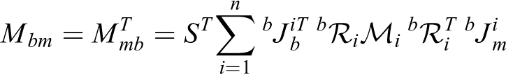
where ${\dot{q}}_r={\left[{\eta }_b^{{\rm T}} {\dot{q}}_m^{{\rm T}}\right]}^{{\rm T}}$ and $\tau ={\left[{\tau }_b^{{\rm T}} {\tau }_m^{{\rm T}}\right]}^{{\rm T}}$ . Mass matrix $M_r(q_m)$ may be determined from

$M_r(q_m)=\left[\begin{array}{cc}{M}_{bb}& M_{bm}\\ M_{mb}& M_{mm}\end{array}\right]$

12

of which

$M_{bb}=S^{{\rm T}}\left({\mathcal{M}}_b+{\displaystyle \sum _{i=1}^n}{}^b{J}_b^{i{\rm T}}{}^b{\mathcal{R}}_i{\mathcal{M}}_i{}^b{\mathcal{R}}_i^{{\rm T}}{}^b{J}_b^i\right)S$

$M_{bm}=M_{mb}^{{\rm T}}=S^{{\rm T}}{\displaystyle \sum _{i=1}^n}{}^b{J}_b^{i{\rm T}}{}^b{\mathcal{R}}_i{\mathcal{M}}_i{}^b{\mathcal{R}}_i^{{\rm T}}{}^b{J}_m^i$

$M_{mm}={\displaystyle \sum _{i=1}^n}{}^b{J}_m^{i{\rm T}}{}^b{\mathcal{R}}_i{\mathcal{M}}_i{}^b{\mathcal{R}}_i^{{\rm T}}{}^b{J}_m^i$

Coriolis/centrifugal matrix $C_r(\epsilon ,q_m,{\dot{q}}_r)$ may be derived from the terms $M\ddot{q}+C\dot{q}$ in (9) by applying (2), (10), and using $\text{diag}{\left(S(\epsilon ),I_{n\times n}\right)}^{{\rm T}}$ to map the related torque. Gravitational torque $G_r(\epsilon ,q_m)$ may be computed through $G=\partial \mathcal{U}/\partial q$ and $G_r=\text{diag}{\left(S(\epsilon ),I_{n\times n}\right)}^{{\rm T}}G$ .

Momentum minimization

Generalized momentum vector P is defined as $P(q,\dot{q})\triangleq \partial {\mathcal{T}}^{*}/\partial \dot{q}=M(\epsilon ,q_m)\dot{q}$ . Dynamically, it indicates the signed accumulation of the applied torque onto the system. Therefore, minimizing the momentum tends to minimize the area under the torque-time graph. Regarding the motion of a multi-DOFs robot, the parts tend to move in opposite direction to each other such that their corresponding momentums cancel and thus minimizing the total momentum. Physically, linkages move cooperatively during locomotion, and corresponding torque required to execute the motion will be incurred to all joints. Hence, the robot is capable of performing challenging motion by proper internal movement as demonstrated in the video ^5,6 since its torque capacity has been fully utilized. On the other hand, because $\mathcal{T}(q,P)\triangleq P^{{\rm T}}M{(q)}^{-1}P/2$ is the robot kinetic energy, minimizing the magnitude of P weighted by $M^{-1}$ implies minimizing the kinetic energy supplied to the robot. Experimental results of natural locomotion in the literature ^3,4 support this proposition. From these reasonings, weighted momentum minimization is a viable criteria to resolve the robot redundancy that yields many interesting optimal characteristics.

Control of the robot locomotion to follow desired trajectory while globally minimizing the weighted generalized momentum may be casted as an optimal control problem

$\text{arg}\underset{\tau (t)}{{\displaystyle \text{min}}}{\displaystyle {\int }_0^T}\frac{1}{2}{\dot{q}}^{{\rm T}}M{(q)}^{{\rm T}}W(q)M(q)\dot{q} \text{d}t$

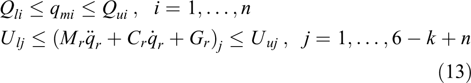
subject to (3), (9), and $X(q,t)=0$ of d-desired trajectory constraints. Since the robot locomotion problem concerns specifying the platform coordinates $q_b(t)$ , desired trajectory constraints may be explicitly written as $X(q_b,t)=0$ . Weighting matrix $W(q)\succcurlyeq 0$ imposes different weighting or penalty for each component of P. Note that the optimization is global which does not incur the stability problem during long-time trajectory generation. ^11,13 In practice, robots have joint angle and actuator torque lower and upper limits, while the joint velocity limit is hardly encountered and thus will be ignored. These inequality constraints may be expressed as

$\begin{array}{l}{Q}_{li}\le q_{mi}\le Q_{ui}, i=1,\dots ,n\\ U_{lj}\le {(M_r{\ddot{q}}_r+C_r{\dot{q}}_r+G_r)}_j\le U_{uj}, j=1,\dots \mathrm{,6}-k+n\end{array}$

13

for the manipulator n-joint angle limits and all the robot $(6-k+n)$ -actuator torque limits. They may be accounted for in the optimal control problem via the Lagrange multipliers.

On minimizing the momentum during locomotion, joint angles will encounter their limits at some instant. In turn, large values of Lagrange multipliers will be induced. Thus, significant counter-torque must be applied to prevent the joint motion from exceeding the limit. Required torque might at worst exceed the actuator torque limit. Even if it still resides in the bound, the magnitude is likely to become unacceptably large. There are several methods to prevent this situation, however. One might employ passive dissipation mechanism to damp out massive energy instead of using the actuator to play the role in impeding the motion. Another is to insert the spring and damper around the manipulator joints in order to keep the arm around a suitable posture away from the joint limits, which also serves as the resting posture after the locomotion has finished. In biological systems, tendons and cartilages around the joints are elements that function as such. However, it would be more convenient for the robot system to implement the spring and damper elements via programmable actuator torques.

Minimization of new Lagrangian

Spring force around the manipulator resting posture $q_{m_e}$ during optimal locomotion may be achieved by minimizing the exchange between the momentum cost, ${\dot{q}}^{{\rm T}}{M}^{{\rm T}}WM\dot{q}/2$ , and the new potential energy, ${\left(q_m-q_{m_e}\right)}^{{\rm T}}{K}_p\left(q_m-q_{m_e}\right)/2$ , with $K_p\succcurlyeq 0$ . The resulting motion resembles human natural locomotion in a manner that the limbs deviate more from their resting pose as the trunk accelerates. Pull-back spring forces will prevent the limbs from moving too fast. From the energy viewpoint, part of the kinetic co-energy is transferred to the spring potential. Conversely, when the trunk decelerates, the limbs approach the resting pose by reclaiming the stored potential energy back to the kinetic co-energy. Additionally, if the trunk needs to accelerate in a short period, the stored energy may be retrieved immediately as an extra power helping propel aggressively. For this case, the limbs energetically swing back toward the resting pose as the trunk dynamically moves forward.

Associated joint damping force, $K_d{\dot{q}}_m$ , with $K_d\succcurlyeq 0$ is introduced as another means to preclude the joint motion from exceeding the limit and to suppress elastic vibration. The optimal problem may now be viewed as globally minimizing the difference of the robot’s weighted generalized momentum and the assigned potential energy

${\mathcal{L}}_n=\frac{1}{2}{\dot{q}}^{{\rm T}}M{(q)}^{{\rm T}}W(q)M(q)\dot{q}-\frac{1}{2}{\left(q_m-q_{m_e}\right)}^{{\rm T}}{K}_p\left(q_m-q_{m_e}\right)$

or the new Lagrangian ${\mathcal{L}}_n(q,\dot{q})$ , subject to (9), $X(q_b,t)=0$ , (13), (3), and $K_d{\dot{q}}_m$ .

Optimal torque ${\tau }^{*}(t)$ may be determined by solving the two-point boundary value problem (TPBVP) which usually is computationally intensive and so cannot be done in real time. Rather than searching for ${\tau }^{*}(t)$ , the optimal control problem may be viewed as to determine the corresponding optimal trajectory $q^{*}(t)$ which extremize the integral

$\mathcal{I}\triangleq {\displaystyle {\int }_0^T}\mathcal{Q}(q,\dot{q},\ddot{q},t)dt$

subject to the platform constraints and damping force. Instantaneous cost addressing the new Lagrangian, desired trajectory constraints, and joint angle and actuator torque limits is

$\begin{array}{c}\mathcal{Q}(q,\dot{q},\ddot{q},t)={\mathcal{L}}_n(q,\dot{q})+{\displaystyle \sum _{c=1}^d}{\mu }_c{X}_c(q,t)\\ +{\displaystyle \sum _{i=1}^n}{\mu }_{p_{li}}\left[-{\ddot{q}}_{mi}-\left({\kappa }_{1i}+{\kappa }_{2i}\right){\dot{q}}_{mi}-{\kappa }_{1i}{\kappa }_{2i}\left(q_{mi}-Q_{li}\right)\right]\\ +{\displaystyle \sum _{i=1}^n}{\mu }_{p_{ui}}\left[{\ddot{q}}_{mi}+\left({\kappa }_{1i}+{\kappa }_{2i}\right){\dot{q}}_{mi}+{\kappa }_{1i}{\kappa }_{2i}\left(q_{mi}-Q_{ui}\right)\right]\\ +{\displaystyle \sum _{j=1}^{6-k+n}}{\mu }_{a_{lj}}\left[-M_{rj}{\ddot{q}}_r-C_{rj}{\dot{q}}_r-G_{rj}+U_{lj}\right]\left(\epsilon ,q_m,\dot{q},\ddot{q}\right)\\ +{\displaystyle \sum _{j=1}^{6-k+n}}{\mu }_{a_{uj}}\left[M_{rj}{\ddot{q}}_r+C_{rj}{\dot{q}}_r+G_{rj}-U_{uj}\right]\left(\epsilon ,q_m,\dot{q},\ddot{q}\right)\end{array}$

14

using the Lagrange multipliers ${\mu }_c$ for the $c\text{th}$ -desired trajectory constraint, ${\mu }_{p_{li}}$ / ${\mu }_{p_{ui}}$ for the ith-joint angle lower/upper limit, and ${\mu }_{a_{lj}}$ / ${\mu }_{a_{uj}}$ for the jth-actuator torque lower/upper limit. Here, torque constraints are expressed as function of $\left(\epsilon ,q_m,\dot{q},\ddot{q}\right)$ instead of $\left(\epsilon ,q_m,{\dot{q}}_r,{\ddot{q}}_r\right)$ to comply with the generalized coordinates q of the Lagrange formulation. Subscript j of M_r , C_r , and G_r denotes their jth-row.

Note the original joint angle limit (13) is modified to

${\kappa }_{1i}{\kappa }_{2i}{Q}_{li}\le {\ddot{q}}_{mi}+({\kappa }_{1i}+{\kappa }_{2i}){\dot{q}}_{mi}+{\kappa }_{1i}{\kappa }_{2i}{q}_{mi}\le {\kappa }_{1i}{\kappa }_{2i}{Q}_{ui}$

15

using the Gronwall inequality so that it is related directly to the acceleration or torque. Equation (15) is more restrictive than (13) since if $q_{mi}$ merely converge to $Q_{li}$ or $Q_{ui}$ with the rate exceeding some value proportional to ${\kappa }_{1i}$ and ${\kappa }_{2i}$ , (15) will become active. Hence, the joint angle limit is represented by (15). Note that fast convergent rate with ${\kappa }_{1i}$ and ${\kappa }_{2i}\gg 1$ calls for $|U_{li}|$ and $|U_{ui}|\gg 1$ to protect the joint limit intrusion. Indeed, (13) implies that the motion must be stopped immediately as $Q_{li}$ or $Q_{ui}$ has reached, which is not possible since this requires infinite acceleration or deceleration.

Optimal trajectory generation

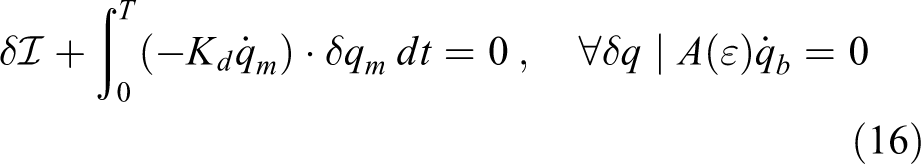
The optimal problem formulation of determining $q^{*}(t)$ resembles the Hamilton’s principle of least action, for which calculus of variation ¹⁷ may be applied. Specifically, $q^{*}(t)$ will be the function that satisfy

$\delta \mathcal{I}+{\displaystyle {\int }_0^T}\left(-K_d{\dot{q}}_m\right)\cdot \delta q_{m}dt=0,\forall \delta q | A(\epsilon ){\dot{q}}_b=0$

16

and $\delta q(0)=\delta q(T)=0$ , $\delta \dot{q}(0)=\delta \dot{q}(T)=0$ . Evaluating (16), $q^{*}(t)$ must satisfy the following differential equations

$\frac{\partial \mathcal{Q}}{\partial q}-\frac{d}{dt}\left(\frac{\partial \mathcal{Q}}{\partial \dot{q}}\right)+\frac{d^2}{d{t}^2}\left(\frac{\partial \mathcal{Q}}{\partial \ddot{q}}\right)=\left[\begin{array}{c}-A{(\epsilon )}^{{\rm T}}\lambda \\ K_d{\dot{q}}_m\end{array}\right]$

17

Substituting $\mathcal{Q}(q,\dot{q},\ddot{q},t)$ of (14) into (17), one has

$\begin{array}{l}{M}^{{\rm T}}WM\ddot{q}+\frac{d}{dt}\left(M^{{\rm T}}WM\right)\dot{q}\\ -{\left[\begin{array}{c}{0}_{3\times 1}\\ \frac{1}{2}{\dot{q}}^{{\rm T}}\frac{\partial }{\partial q_i}\left(M^{{\rm T}}WM\right)\dot{q}\end{array}\right]}_{i=4 \text{to} 7+n}+\left[\begin{array}{c}{0}_{7\times 1}\\ K_d{\dot{q}}_m+K_p\left(q_m-q_{m_e}\right)\end{array}\right]\\ -\left[\begin{array}{c}{0}_{7\times 1}\\ \left({\ddot{\mu }}_{p_u}-{\ddot{\mu }}_{p_l}\right)-\left({\kappa }_1+{\kappa }_2\right)\left({\dot{\mu }}_{p_u}-{\dot{\mu }}_{p_l}\right)+{\kappa }_1{\kappa }_2\left({\mu }_{p_u}-{\mu }_{p_l}\right)\end{array}\right]\\ -E\left({\ddot{\mu }}_{a_u}-{\ddot{\mu }}_{a_l}\right)-\ddot{E}\left({\mu }_{a_u}-{\mu }_{a_l}\right)+D\left({\dot{\mu }}_{a_u}-{\dot{\mu }}_{a_l}\right)\\ +\dot{D}\left({\mu }_{a_u}-{\mu }_{a_l}\right)-\left[\begin{array}{c}{0}_{3\times (s+n)}\\ B\end{array}\right]\left({\mu }_{a_u}-{\mu }_{a_l}\right)=J^{{\rm T}}\mu +\left[\begin{array}{c}A{(\epsilon )}^{{\rm T}}\lambda \\ 0_{n\times 1}\end{array}\right]\end{array}$

18

of which

$\begin{array}{l}{\text{col}}_j(B)=\frac{\partial M_{rj}}{\partial q_{4 \text{to} 7+n}}{\ddot{q}}_r+\frac{\partial C_{rj}}{\partial q_{4 \text{to} 7+n}}{\dot{q}}_r+\frac{\partial G_{rj}}{\partial q_{4 \text{to} 7+n}}\\ {\text{col}}_j(D)=\frac{\partial C_{rj}}{\partial \dot{q}}{\dot{q}}_r+{\left(\frac{\partial {\dot{q}}_r}{\partial \dot{q}}\right)}^{{\rm T}}{C}_{rj}^{{\rm T}} , j=1,\dots \mathrm{,6}-k+n\\ E={\left(\frac{\partial {\ddot{q}}_r}{\partial \ddot{q}}\right)}^{{\rm T}}{M}_r,J{(q_b)}^{{\rm T}}={\left(\frac{\partial X}{\partial q}\right)}^{{\rm T}}\\ {\left(\frac{\partial {\dot{q}}_r}{\partial \dot{q}}\right)}^{{\rm T}}={\left(\frac{\partial {\ddot{q}}_r}{\partial \ddot{q}}\right)}^{{\rm T}}=\text{diag}\left(S{(\epsilon )}^{-{\rm T}},I_n\right)\end{array}$

and ${\mu }_{p_l}/{\mu }_{p_u}$ , ${\mu }_{a_l}/{\mu }_{a_u}$ , μ, and λ are Lagrange multiplier vectors for joint angle, actuator torque limits, desired trajectory, and platform motion constraints, respectively. In the following, the optimal system dynamics will be derived and a method to determine the optimal trajectory online is proposed.

Optimal system dynamics

Combining (18) with $X(q,t)=0$ , (3), (15), and (13) results in the differential-algebraic equations (DAEs). The system has q, ${\mu }_{p_l}$ , ${\mu }_{p_u}$ , ${\mu }_{a_l}$ , ${\mu }_{a_u}$ as second-order differential variables and μ, λ as algebraic variables. Since the desired trajectory and platform motion constraints should be satisfied at all time, they may in turn be differentiated twice and once to obtain their acceleration-level equations

$\ddot{X}(q,\dot{q},\ddot{q},t)=0$

19

$A(\epsilon ){\ddot{q}}_b+{\displaystyle \sum _{i=0}^3}\frac{\partial A(\epsilon )}{\partial {\epsilon }_i}{\dot{\epsilon }}_i {\dot{q}}_b=0$

20

As a result, the DAEs are transformed into the ordinary differential equations (ODEs) that are much easier to solve. Furthermore, they may be stabilized using the method of Baumgarte ¹⁸ to alleviate the constraint drift caused by numerical integration.

At any instant, each inequality of (15) and (13) has three possible status; inactive, lower limit, or upper limit active. Each of these is equipped with different constraints, and hence constitutes different dynamics as a part of the optimal hybrid system. Suppose the jth-inequality of the actuator torque limits is inactive. For this case, there is no associated constraint and

${\ddot{\mu }}_{a_{lj}}=0{\ddot{\mu }}_{a_{uj}}=0$

with zero initial conditions. However, if the inequality is lower limit active, the constraint

$-M_{rj}{\ddot{q}}_r-C_{rj}{\dot{q}}_r-G_{rj}+U_{lj}=0$

from (13) requires that ${\ddot{\mu }}_{a_{uj}}=0$ with zero initial conditions. ${\mu }_{a_{lj}}$ may be determined from the dynamics according to this constraint with initial conditions taken from the values of the previous time step. This is the extension of Pontryagin’s minimum principle ¹⁹ where both the Lagrange multipliers and their time derivatives are involved in the equations of motion. If the ith-inequality of the joint angle limits is lower limit active, the constraint

$-{\ddot{q}}_{mi}-({\kappa }_{1i}+{\kappa }_{2i}){\dot{q}}_{mi}-{\kappa }_{1i}{\kappa }_{2i}(q_{mi}-Q_{li})=0$

from (15) requires ${\ddot{\mu }}_{p_{ui}}=0$ with zero initial conditions. ${\mu }_{p_{li}}$ is determined from the dynamics associated with this constraint. Inequality with upper limit active may be formulated similarly.

Since there are $(6-k+2n)$ -inequality constraints in (15) and (13), at any instant the system will evolve along one of the $3^{6-k+2n}$ possible dynamics. The dynamics may switch from one to another as the status of (15) and (13) change; a hybrid system. It is evident that the number of possible dynamics could well be overabundant whereas many of them might never happen during the course. Therefore, an analysis should be performed for each particular system in order to rule out the constraint combinations and dynamics that are unlikely to happen.

Some dynamics may possess inconsistent ODEs caused by the conflicts among constraints. Thus, it cannot be solved unless the cost or constraints are modified, or some task requirements are removed temporarily. In this work, conflicting dynamics are handled by relaxing some desired trajectory constraints through setting the respective ${\mu }_c=0$ , such that the remaining constraints can be satisfied.

In summary, (18) to (20), (15), (13), and the corresponding zero-Lagrange multiplier ODEs constitute the optimal hybrid system dynamics that globally minimize ${\mathcal{L}}_n$ subject to the desired trajectory and platform motion constraints, joint angle and actuator torque limits, as well as the manipulator’s joint damping force. If the virtual spring and damper are strong enough and the actuator torque limits are adequate to supply the required force, all joint angle and torque limits will be inactive. In that case, (18) becomes

$\begin{array}{l}{M}^{{\rm T}}WM\ddot{q}+\frac{d}{dt}\left(M^{{\rm T}}WM\right)\dot{q}-{\left[\begin{array}{c}{0}_{3\times 1}\\ \frac{1}{2}{\dot{q}}^{{\rm T}}\frac{\partial }{\partial q_l}\left(M^{{\rm T}}WM\right)\dot{q}\end{array}\right]}_{l=4 \text{to} 7+n}\\ +\left[\begin{array}{c}{0}_{7\times 1}\\ K_d{\dot{q}}_m+K_p\left(q_m-q_{m_e}\right)\end{array}\right]=J^{{\rm T}}\mu +\left[\begin{array}{c}A{(\epsilon )}^{{\rm T}}\lambda \\ 0_{n\times 1}\end{array}\right]\end{array}$

21

and the inequality (15) and (13) yield ${\ddot{\mu }}_{p_{li}}$ , ${\ddot{\mu }}_{p_{ui}}$ , ${\ddot{\mu }}_{a_{lj}}$ , ${\ddot{\mu }}_{a_{uj}}=0$ with zero initial conditions. Implicitly, the optimal system is not any more hybrid and its dynamics is greatly simplified.

Online determination of the optimal trajectory

Optimal motion $q^{*}(t)$ may be determined online as part of solving the optimal dynamics for differential and algebraic variables. Since the system is hybrid, its dynamics may be changing which is not known a priori. Therefore, the inequality constraint status, corresponding system dynamics, and the solution must be determined altogether. A procedure to solve this problem is proposed. First, a constraint status is assumed. System dynamics can then be determined and solved based upon the assumption. According to the solution, the constraint status will be examined if it agrees with what has been assumed. Specifically, for each numerical time step:

Initially, assume no active inequality constraint. Solve the corresponding dynamics.

Examine the constraint status of the solution. If it is as what has been assumed, the optimization is solved for this time step.

If the status contradicts the assumption, adopt it as a new postulate. Solve the new dynamics.

Reevaluate steps 2 and 3 until the status of the solution agrees with the assumed one.

It should be noted that in order to prevent the joint range violation, active joint angle limit may induce active joint torque limit. However, the latter constraint might not be detected at the same iteration as the former. On the other hand, if the robot is equipped with powerful enough actuators, the joint torque limit may not happen. In general, activation of (15) and (13) depends on several factors; desired trajectory, W, K_p , K_d , and values of the limit themselves. Careful selection helps avoid the constraints, which simplifies determining the optimal trajectory.

To solve the optimal dynamics in the most general setting, the $(20+5n+d-k)$ -variables of $\ddot{q}$ , ${\ddot{\mu }}_{p_l}$ , ${\ddot{\mu }}_{p_u}$ , ${\ddot{\mu }}_{a_l}$ , ${\ddot{\mu }}_{a_u}$ , μ, λ will be extracted from each ODE and collected in that order as a column-tuple Y. For example, (18) having $(7+n)$ -ODEs may be arranged as

$\begin{array}{l}\left[\begin{array}{ccccccc}{M}^{{\rm T}}WM& \begin{array}{c}{0}_{7\times n}\\ I_{n\times n}\end{array}& \begin{array}{c}{0}_{7\times n}\\ -I_{n\times n}\end{array}& E& -E& -J^{{\rm T}}& \begin{array}{c}-A{(\epsilon )}^{{\rm T}}\\ 0_{n\times (k+1)}\end{array}\end{array}\right]Y\\ =-\frac{d}{dt}\left(M^{{\rm T}}WM\right)\dot{q}+{\left[\begin{array}{c}{0}_{3\times 1}\\ \frac{1}{2}{\dot{q}}^{{\rm T}}\frac{\partial }{\partial q_l}\left(M^{{\rm T}}WM\right)\dot{q}\end{array}\right]}_{l=4 \text{to} 7+n}\\ -\left[\begin{array}{c}{0}_{7\times 1}\\ K_d{\dot{q}}_m+K_p\left(q_m-q_{m_e}\right)\end{array}\right]+\ddot{E}\left({\mu }_{a_u}-{\mu }_{a_l}\right)\\ -D\left({\dot{\mu }}_{a_u}-{\dot{\mu }}_{a_l}\right)-\dot{D}\left({\mu }_{a_u}-{\mu }_{a_l}\right)+\left[\begin{array}{c}{0}_{3\times (s+n)}\\ B\end{array}\right]\left({\mu }_{a_u}-{\mu }_{a_l}\right)\\ +\left[\begin{array}{c}{0}_{7\times 1}\\ -\left({\kappa }_1+{\kappa }_2\right)\left({\dot{\mu }}_{p_u}-{\dot{\mu }}_{p_l}\right)+{\kappa }_1{\kappa }_2\left({\mu }_{p_u}-{\mu }_{p_l}\right)\end{array}\right]\end{array}$

Combining all ODEs arranged in this form together, Y may now be determined by solving the standard matrix-vector equation $HY=F$ with a square invertible matrix H of the consistent system and a column-tuple F of the same dimension as Y. Numerical integration may then be applied to solve for $q=q^{*}$ , ${\mu }_{p_l}$ , ${\mu }_{p_u}$ , ${\mu }_{a_l}$ , ${\mu }_{a_u}$ , and their first-order derivatives used in the next time step.

After $q^{*}(t)$ has been determined, a robust trajectory tracking controller may be used to compute the required torque with $q^{*}(t)$ as reference trajectory input. Figure 2 depicts the overall system diagram. The optimal controller is divided into two parts; optimal trajectory generator and tracking controller. This is in contrast to the optimal control approach which computes ${\tau }^{*}(t)$ directly by solving a very difficult TPBVP. From the diagram, if the tracking controller can make $q(t)$ follow $q^{*}(t)$ , the robot closed-loop dynamics will match that of the optimal system. By (18), the closed-loop robot is a Lagrangian system that virtually has the generalized mass of $M^{{\rm T}}WM$ , the manipulator joint damping K_d , and joint spring K_p regulating around the resting posture. These parameters may be crafted to achieve desired behavior of the robot. With this new dynamics, the closed-loop robot is subject to the applied torque $J^{{\rm T}}\mu$ required to track the desired trajectory. Additional torque from the 5th to 10th terms in (18) is activated when the joint angle and/or actuator torque limit is violated. Also, the platform constraints exert torque $A{(\epsilon )}^{{\rm T}}\lambda$ that forces the robot to move along (3).

Figure 2.

System diagram indicating the separation between the trajectory generation and the tracking controller. Robot current states are used to compute the adaptive optimal trajectory.

Until now, $q^{*}(t)$ depends on $X(q_b,t)=0$ , but not on $q(t)$ . Numerically, q* and its time derivative of the previous time step act as the initial conditions to solve for q* at the current time step given $q_b(t)$ . q* computed in this way may be regarded as the open-loop optimal trajectory since it does not use feedback of the system states. Implicitly, q is assumed to track q* exactly at every time step. This might not happen in practice due to, for example, the controller or robot unmodeled dynamics. Consequently, q* will merely be the preplanned optimal trajectory. In order to make q* be the real-time updated optimal trajectory reflecting the actual tracking error, it should be determined using the robot current states as the initial conditions at every time step, rather than using the optimal states of the previous time step. This modification is shown in Figure 2 as the dashed line feeding back to the trajectory generation module. q* is now the adaptive optimal trajectory according to the actual system states. An example of the tracking controller is given and the exponential convergence of $q(t)$ to $q^{*}(t)$ is proven in Appendix 1.

The proposed framework can be applied to numerically solve any optimal control problem of the mechanical system online. First, the functions ${\mathcal{L}}_n$ and $\mathcal{Q}$ must be determined. Next, calculus of variation is applied to solve the extremization of the action $\mathcal{I}$ , where a set of ODEs governing the optimal system dynamics is derived. This will be solved for the optimal trajectory, which serves as the input to the tracking controller. The controller will then calculate the torque required to track the optimal trajectory. Such torque is the optimal torque required to optimize ${\mathcal{L}}_n$ globally subject to constraints embedded in $\mathcal{Q}$ by Lagrange multipliers.

Selection of the weighting matrix

Selection of the weighting or penalty matrix W depends on how one would like to exploit the momentum of different robot parts for the purpose of tracking desired trajectory. Weighting values $w_{ij}$ and $w_{ji}$ of the $(i,j)$ and $(j,i)$ -elements in W should be set high if the i and j-generalized momentums, p_i and p_j , will be barely utilized. Then, because $p_i={\displaystyle {\sum }_{k=1}^{7+n}}{m}_{ik}(q){\dot{q}}_k$ , generalized velocities which highly influence the momentum will be of little values. Consequently, motion of the parts pertaining to these velocities will become small. Conversely, if one would like to utilize the motion of a robot part corresponding to the generalized velocity $\dot{q}$ for tracking desired trajectory, its generalized momentum $p=M(q)\dot{q}$ should be computed and the dominant l-component p_l be determined. Thus, weighting elements of W involving p_l should be set to low values as they will incur small penalty on this motion, encouraging the part to move.

Remark that if $W=M^{-1}$ , the closed-loop robot mass will be the same as the open-loop one. This implies that the natural motion, or motion of the open-loop robot itself with no influence from external force, attempts to globally minimize the robot momentum weighted by $M^{-1}$ , which is also the open-loop robot kinetic energy. Hence, by choosing $W=M^{-1}$ , the energy supplied to the robot is the minimal kinetic energy for tracking the desired trajectory. Generally, one can shape the closed-loop robot mass $M_n\succ 0$ arbitrarily by choosing $W=M^{-1}{M}_n{M}^{-1}$ . If M_n is a constant diagonal matrix, the closed-loop dynamics will be fully decoupled. Nevertheless, the weighting should also be chosen taking the robot mass distribution and joint angle/torque limit into account so the optimal trajectory is realizable. Roughly speaking, the more the deviation of M_n from M, the more additional torque is required for mimicking the inertial force of the optimal system.

Simulation

In this section, the proposed optimal locomotion generator and tracking controller (2A) and (3A) are applied to a cart-pole robot. The system in Figure 3 serves as an instructive example since its motion is comparable to gross human locomotion and important results can be observed clearly. The cart mass M is 10 kg while that of the pole m is 5 kg. Its C.G. is located at $l_c=0.3$ m from the joint and the inertia about the C.G. is $I=0.15$ kg m². Because the cart movement is constrained to simple rectilinear motion, desired locomotion of the platform may be specified by $x_d(t)$ with the platform constraint vanished. In other words, $q={\left[x,\theta \right]}^{{\rm T}}$ and the system dimension is reduced to 2. The robot dynamics may be derived as

$A\ddot{x}-B\ddot{\theta }\text{sin}\theta -B{\dot{\theta }}^2\text{cos}\theta ={\tau }_b$

$-B\ddot{x}\text{sin}\theta +C\ddot{\theta }+D\text{cos}\theta ={\tau }_m$

where $A=M+m$ , $B=m{l}_c$ , $C=I+m{l}_c^2$ , $D=mg{l}_c$ , and their numerical values are 15, 1.5, 0.6, and 14.7. ${\tau }_b$ and ${\tau }_m$ are the driving force and linkage torque exerted along the x- and θ-coordinate. Therefore, the robot is redundant and the pole movement in the range $\theta \in [\pi /6,5\pi /6]$ may be exploited to assist the locomotion task.

Figure 3.

A cart-pole robot with the coordinate frames.

Assume ${\tau }_{b_{\text{max}}}=400$ N and ${\tau }_{m_{\text{max}}}=100$ Nm. Set $K_d=15$ Nm s/rad and $K_p=15$ Nm/rad with ${\theta }_e=\pi /2$ rad for the joint spring/damper, and ${\kappa }_{1\theta }={\kappa }_{2\theta }=50$ for the joint limit constraints. The controller gains used are $K=\text{diag}(10,10)$ and $\mathrm{\Gamma }=\text{diag}(5,5)$ . Figure 4 shows the desired locomotion $x_d(t)$ (solid line) which imitates the human C.G. motion during walking with varying footstep lengths for 5 s.

Figure 4.

Robot trajectory, torque, and input work using $W=M^{-1}$ . Solid and dashed lines are for x- and θ-quantities.

Robot trajectory, supplied torque, and work input to the robot are plotted in Figures 4 and 5 using $W=M^{-1}$ and $W=\text{diag}(0.5,0.5)$ . In both cases, the robot is able to track x_d . However, different behaviors are observed. When $W=M^{-1}$ is adopted, the link does not swing much because its inertia is very small compared to the platform. Little contribution to the locomotion can be made by the link and thus natural motion decides not to move the link too much.

Figure 5.

Robot trajectory, torque, and input work using $W=\text{diag}(0.5,0.5)$ to track $x_d(t)$ creeping 1 m each second by 1, 2, 5, 2, and 1 stride successively.

On the other hand, if $W=\text{diag}(0.5,0.5)$ is used, the link will swing much more in opposite direction to ${\ddot{x}}_d$ , in an attempt to minimize the generalized momentum according to the new weighting. This is achieved by intentionally swinging the link with ${\tau }_m\approx 50$ Nm such that the induced coupling force is exploited to assist the locomotion meaningfully. From the graphs, average value of ${\tau }_b$ will be lessened from 200 N when using natural dynamics to 100 N. Moreover, the peak value caused by tracking aggressive locomotion during 2–3 s is reduced from 320 N to 160 N. This indicates that the robot is capable of performing more challenging tasks by utilizing all actuators through internal motion of robot linkages according to minimizing the properly weighted generalized momentum as discussed in the “Selection of the weighting matrix” subsection. Total work driving the robot when natural dynamics is exploited is of course the least among all weightings.

Other parameters play a role in designating the robot closed-loop behavior as well. The aim of joint spring and damper is to prevent and stabilize linkage motion from exceeding the joint limit. Even more, the spring is a crucial element to fast motion in a short period. Yet they contort the momentum minimization objective and its benefits. Joint angle and torque limits affect the robot behavior too. When the constraint is active, abrupt large force is required to prevent constraint violation. This ruins the momentum minimization objective. Therefore, the limits should be high enough so that minimizing the momentum can be truly achieved within the full operating range. Lastly, the robot design itself has an impact on its closed-loop behavior. A guideline might be to design the robot with M close to M_n and to employ desired passive spring/dampers. Thus, the robot natural dynamics will be utilized primarily, together with complementary actuator torque, to execute the task with optimal dynamics in the absence of active inequality constraints.

Conclusions

This article presents a formal method to exploit the movement of the manipulator in assisting the locomotion of the mobile robot platform by globally minimizing the weighted generalized momentum. Resulting cooperative motion of the manipulator and platform induces the coupling force which helps propel the robot. Degree of the utilization may be adjusted through the momentum weighting parameters. Notably, the robot exploits its natural dynamics if $W=M^{-1}$ is chosen. The locomotion is modest and requires minimal input work. On the contrary, additional work is needed using other weightings. With certain weightings that produce suitable coordinating motion patterns, the robot may be able to conquer challenging motion under practical constraints. To summarize, global minimization of the weighted generalized momentum causes the redundant robot to perform specified tasks with desirable behavior governed by newly shaped optimal dynamics subject to motion and actuation constraints.