Sage Journals: Discover world-class research

Abstract

To effectively reduce the mass and simplify the structure of traditional aerial manipulators, we propose novel light cable-driven manipulator for the aerial robots in this article. The drive motors and corresponding reducers are removed from the joints to the base; meanwhile, force and motion are transmitted remotely through cables. Thanks to this design, the moving mass has been greatly reduced. In the meantime, the application of cable-driven technology also brings about extra difficulties for high-precise control of cable-driven manipulators. Hence, we design a nonsingular terminal sliding mode controller using time-delay estimation. The time-delay estimation is applied to obtain lumped system dynamics and found an attractive model-free scheme, while the nonsingular terminal sliding mode controller is utilized to enhance the control performance. Stability is analyzed based on Lyapunov theory. Finally, the designed light cable-driven manipulator and presented time-delay estimation-based nonsingular terminal sliding mode controller are analyzed. Corresponding results show that (1) our proposed cable-driven manipulator has high load to mass ratio of 0.8 if we only consider the moving mass and (2) our proposed time-delay estimation-based nonsingular terminal sliding mode is model-free and can provide higher accuracy than the widely used time-delay estimation-based proportional–derivative (PD) controller.

Keywords

Aerial robots cable-driven manipulator structure design kinematic coupling time-delay estimation (TDE)nonsingular terminal sliding mode (NTSM)

Introduction

In recent years, unmanned aerial vehicles (UAVs), as a kind of aerial robots, have been developing toward miniaturization. Especially, multi-rotor aircraft have been widely applied to many fields, such as aerial photography, monitoring, detection and patrol due to their simple structure, flexibility, and low cost.^1

–4 However, with the increasing demand for aerial manipulations, such as bridge inspection and high-voltage electric lines inspection and intelligent manufacturing,^5

–9 most of the existing UAVs cannot meet the needs because they can only be capable of observations.¹⁰ Thus, researchers started to work on UAVs with manipulators.^11
–13

Research studies on operational UAVs have yielded a lot of achievements. The AEROARMS Project developed an aerial robotic manipulator with dual arms for outdoor detection and maintenance.¹⁴ To solve the problem of insufficient load capacity of UAVs, a commercial UAV was combined with a lightweight prototype three-arm manipulator and a motion capture system was used to solve the instability problem of rotorcraft.¹⁵ A UAV developed for bridge inspection was presented and a three-degree-of-freedom (DOF) robot arm was installed on the top of UAV body. Researchers hope this UAV will be able to replace humans in bridge inspecting.¹⁶ By carefully analyzing above works, we can see that all the manipulators used for UAVs are limited within traditional rigid structure. Drive motors and reducers are directly installed in the joints which lead to large moving mass and also disturbance for the UAVs. To solve abovementioned issues, scholars started using lighter robotic arms and the cable-driven manipulator. Motors, reducers, and other drive units can be placed on the base thanks to the cable-driven technology, which means the moving mass and energy consumption can be substantially reduced. To this end, we present a light cable-driven manipulator for UAVs named Polaris-III in this work. Due to its novel structure, the Polaris-III can be utilized independently in both self-developed UAVs and commercial UAVs.

The cable-driven manipulator reduces weight and simplifies structure indeed, but it also brings about control and motion planning problems at the same time.^17

–21 System becomes more sensitive to external interference, and the vibrations of cables strengthen unmodeled dynamics because of low stiffness. These problems will seriously affect the control accuracy and hence many studies have been done. A control strategy that combines gain scheduling and model reference adaptive control was proposed for the mobile manipulation using UAVs.¹⁴ A feedback control law was used to validate the dynamical model of an aerial manipulator equipped in a quad-rotor vehicle. The model was established by introducing the dual quaternion in mathematics.²² To realize the navigation control of aerial robot, dynamical model of a UAV equipped with a robotic arm was formulated using Newton–Euler method. Furthermore, four classical PID controllers were used for the control of UAV’s attitude and altitude.²³ A novel UAV was developed for bridge inspection, and researchers modeled the impact force using Hertzian contact stress to ensure a steady contact between the UAV and the corresponding surface. The reported control strategy is divided into attitude and position-force control, and both of them are PID control.¹⁶ By observing above works, we can see that almost all of them are either model-based control strategies or simple PID control. Considering the unknown system dynamics and complex couplings between manipulators and UAV during operations, accurate dynamic model of cable-driven manipulators are complicated and almost impossible to obtain. Meanwhile, simple PID control usually is not robust enough to ensure high control performance under lumped uncertainties. What we require for aerial manipulation using UAV and manipulator is a simple but effective control scheme.

Time-delay estimation (TDE) technology is a simple but effective way to obtain system dynamics, and thus it is particularly suitable for cable-driven manipulators. The core idea of TDE is to estimate the current system dynamics using intentionally time-delayed system signals, which brings an attractive model-free scheme. As long as the time interval is small enough (usually one or several sampling periods), the estimation error will be within the acceptable range. TDE has been widely used in the field of system state observation and control,^24

–27 such as nonlinear networked control systems,²⁸ robot manipulators,^29

–33 static neural networks,³⁴ and chaos systems.³⁵ To obtain satisfactory control performance, TDE is often combined with other robust control methods. Thanks to its model-free nature, the obtained TDE-based robust control is usually simple and effective. Usually, sliding mode (SM) control is selected to combine with TDE benefiting from its simple structure and strong robustness.

SM control has been widely used in many systems because of its fast response and strong robustness.^36

–41 To ensure finite-time convergence in the SM phase, terminal sliding mode (TSM) with a nonlinear sliding surface was proposed and investigated. To solve the singularity issue in TSM, two methods were proposed. One is to switch the SM surface near the singularity, and the other is to use the nonsingular SM surface directly.⁴² By combining SM control with other theories, such as fraction-order calculus theory,^43
–45 the controller can be effectively improved for high-precision control in various fields. The SM controller with optimized parameters by genetic algorithm had been used in DC-DC converters.⁴⁶ A discrete-time fractional order TSM controller was developed for linear motor.⁴⁷ In the face of complex aerodynamic disturbances, such as wind gust, dissipative drag, and sideslip aerodynamics, an integral SM was added to a novel robust backstepping-based controller. And no need for more information about the model, the chattering-free SM can compensate for disturbances mentioned above ⁴⁸. In addition, particle swarm optimization,⁴⁹ super-twisting algorithm,^50
–52 and fuzzy control theory⁵³ are also often used in SM control. In this article, for the precise control of our proposed cable-driven manipulator Polaris-III, we propose a TDE-based nonsingular TSM (TDE-NTSM) controller. According to the simulation results, in the face of external torque disturbance and sensor measurement noise, the new controller performs better than the traditional TDE-based PD (TDE-PD) controller.

In the rest of this article, the structure of our designed cable-driven manipulator named Polaris-III will be presented in the second section. And kinematic coupling problems between two joints are analyzed in the third section. In the fourth section, controller design and comparative simulations are developed. Finally, the conclusions are presented in the fifth section.

Structure design

As a UAV-oriented cable-driven manipulator, simplicity and lightness are the primary design requirements. Considering the UAV’s own degree of freedom, we designed a 3-DOF planar manipulator named Polaris-III. The overall structure of Polaris-III is shown in Figure 1, and Table 1 presents its main parameters.

Figure 1.

Overall structure of Polaris-III: (a) Combination of designed cable-driven manipulator with a UAV and (b) detailed design of the proposed cable-driven manipulator.

Table 1.

Main parameters of Polaris-III.

Parameter	Value
Max length	421 mm
Mass	875 g
Max payload	120 g
Range of joint angle	±90°
Drive motors (Vishan)	ECG1630
Planetary reducer (Vishan)	SP160710-1223-5490
Encoder	18M-1024-2MD-A40-15-00E

We can see from Figure 1 that the manipulator consists of three parallel joints, each of which uses two cables to control a rotation in two directions (red and blue lines represent two cables of the same joint). All of the drive motors are placed in the base, and only angle measuring encoders are installed on joint shafts which greatly reduce the mass of moving part of Polaris-III. To further minimize mass, 3D-printed nylon material is widely used in the manipulator. In addition, joint shafts and linkages, such important parts, are aluminum alloy. To prevent cables from escaping from guiding wheels and reduce the friction, we designed spiral grooves and corresponding cable tensioning mechanism which will be explained in detail later.

The main parameters are shown in Table 1; the appropriate length of Polaris-III can bring about its large workspace. Also, the total mass is only about 875 g by simplifying the structure and using lightweight materials. However, the maximum of load to mass ratio is up to 0.14 and this value can reach more than 0.8 if we only consider the moving mass. Note that the proposed cable-driven manipulator can only move in 2-DOF, which is applied to simplify the system structure. Meanwhile, the UAV can provide the working ability for other directions.

Combination of designed cable-driven manipulator with a UAV.

Detailed design of the proposed cable-driven manipulator.

In practice, the smaller the mass ratio between manipulators and UAVs is, the smaller the disturbance to UAVs caused by the movement of manipulators will be. Most of the time, a manipulator’s base is fixed with a UAV, which means the moving part mass is very small compared to that of UAVs. So disturbances to a UAV during operations of the manipulator almost can be ignored. Another benefit of lightweight is the decrease of energy consumption. We all know that limited working hours are an important factor limiting the development of UAV, so lower energy consumption can increase endurance. Lightweight manipulators require fewer loads on UAVs, which can grab heavier targets with the same load capacity. These are the superiorities of the designed cable-driven manipulator applied to an aerial robot.

As mentioned earlier, a tensioning mechanism was designed to prevent the rope from loosening. Moreover, to avoid friction between the cables, the cable grooves on joint wheels and guiding wheels are designed in a spiral structure. And these structures are not visible in Figure 1. Hence, the following are detailed instructions on cable winding method and tensioning mechanism of Polaris-III.

Because driving cables can only withstand tension, two cables are necessary for a motor to control the joint rotation in two directions. Taking joint 2 as an example to explain the winding method of driving cables. As shown in Figure 2, the red line is the cable that controls clockwise rotation of joint 2 (observing from the right) and the blue line represents the driving cable in the other direction. First, the red cable starts at the anchor point on driving wheel-2, goes clockwise around driving wheel-2, and then wraps about 360° around guiding wheel-1 counterclockwise. Then the red cable goes around two tensioning wheels in opposite directions and wraps around joint wheel-2 counterclockwise. This completes the winding arrangement of a driving cable. The blue rope is wound in a similar way, but in opposite direction.

Figure 2.

Winding method of joint 2 driving cables.

As we can see, the forward and backward rotation of joint 1 will cause driving cable of joint 2 to wind and disengage on guiding wheel-1. When the manipulator is in the initial position, depicted in Figure 1, the cable must wind more than 90° on the guiding wheel to stop it from disengaging. Therefore, we wound about 360°. However, the problem yet to be solved in this design is that the driving wheel and guiding wheel have different radii, which means that the angle of winding on driving wheel is different from the angle of disengaging from guiding wheel. Even though the spiral grooves on two wheels have the same pitch, it also causes cables and grooves no longer to fit perfectly, thus, causing unnecessary friction.

After winding, we must elaborate on the designed tensioning mechanism. To ensure the precision of Polaris-III, driving cables should not relax during operations. So it is necessary to design tensioning mechanisms for cable-driven manipulators. Taking joint 2 to analyze, as depicted in Figure 3, driving cables wind through two tensioning wheels in opposite directions, and the tensioning wheel will be fixed on the tensioning frame by friction if the fixed bolt is tightened. And when the driving cable relaxes, loosen the fixed bolt, then tensioning wheels can be adjusted along the direction perpendicular to the linkage. Thus, the driving cable can be tightened again.

Figure 3.

Tensioning mechanism of joint 2.

Different from joint 2 and joint 3, joint 1 has its own tensioning scheme which contains only one tensioning wheel because there is no space to put the tensioning mechanism like other two joints. Fixed on the upper support plate of the base by a bracket, the tensioning wheel controls tightness of joint 1 driven cable by moving back and forth, which can be seen from Figure 4.

Figure 4.

Tensioning mechanism of joint 1.

However, two tensioning mechanism like this still need to be improved for two reasons. First, in practice, such a mechanism cannot be conveniently adjusted because these components are too small. And the tension of cables after adjustment is completely controlled by human experience, so it is impossible to accurately obtain the desired tension. Second, the repeated winding of driving cables on two tensioning wheels in the opposite direction is likely to cause fatigue fracture problems. Hence, we will try to improve the tensioning mechanism in the future.

We describe the overall structure and main parameters of the designed Polaris-III in this section. The winding method of driving cables and the design of tensioning mechanism are explained emphatically. Although they still have problems to be solved, however, do not affect the current use.

Thanks to abovementioned structure, small moving inertia and low-energy consumption can be guaranteed. In the next step, we will build up our first prototype to test the effectiveness of the proposed new structure and decoupling method.

Coupling analysis

Unlike traditional rigid robotic arms, there exists kinematic coupling problem between two joints of a cable-driven manipulator due to the introduction of cable-driven technology. Kinematic coupling is that even if the driving motor of joint i does not rotate, the motion of joint j will still cause additional motion of joint i. Kinematic coupling makes the motion of each joint related to each other, which is very unfavorable to the precise tracking control of the cable-driven manipulator. Moreover, if the joint coupling problem exists in a robot arm, it must be considered in the motion planning because the result of motion planning after inverse kinematics solution is the desired trajectory of each joint in joint space which will subject to the joint coupling. Hence, the coupling problem must be analyzed and compensated.

It is necessary to present some assumptions before analyzing the kinematic coupling problem.^54,55 First, the driving cables of all joints are always tensioned and the change of cable length is ignored because the cable has great stiffness. Second, since one end of the cable is attached to the driving wheel, the relative sliding between the cable and the driving wheel is negligible.

For the sake of simplicity, we will only analyze the coupling between two adjacent joints, and the coupling between other joints can be obtained by analogy.

In Figure 5, a schematic diagram of a 2-DOF cable-driven manipulator, the solid line shows where the links are before joint i rotates, and the dotted line shows the position of link i and link i + 1 after the rotation. The red line is the driving cable for joint i and the blue line is for joint i + 1. And one end of the red cable is fixed on wheel connected with motor shaft and the other end is fixed on joint wheel i after winding several guiding wheels. The difference is that the blue cable wrapped around an extra guiding wheel.

Figure 5.

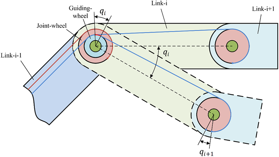
Schematic diagram of kinematic coupling between two adjacent joints.

As depicted in Figure 5, joint i was driven by the motor to rotate clockwise by angle q_i , and we can see that this causes the blue cable to wind around the guiding wheel for angle q_i . Since the drive motor of joint i + 1 was not working, the excess cable wound around guiding wheel means that the cable must detached from joint wheel i + 1. Thus, joint i + 1 rotated angle $q_{i + 1}$ counterclockwise with respect to link i. The cable is assumed to be tensed and not to slide relative to wheels. Therefore, the length of cable wound on the guiding wheel should be the same as the length of cable detached from the joint wheel and we can get the following equation

r_{g}^{i} q_{i} = r_{j}^{i + 1} q_{i + 1}

where $r_{g}^{i}$ represents the radius of the guiding wheel i, and $r_{j}^{i + 1}$ stands for the radius of the joint wheel i + 1. To eliminate the additional rotation due to kinematic coupling, the motor should drive joint i + 1 to rotate clockwise by angle ${q^{'}}_{i + 1}$

{q^{'}}_{i + 1} = q_{i + 1} = \frac{r_{g}^{i}}{r_{j}^{i + 1}} q_{i}

This conclusion is based on the premise that the driving cable is wound in the same direction on the joint wheel and the guiding wheel. In other words, if the blue cable in Figure 5 is wound counterclockwise on joint wheel i + 1, then the motor must control joint i + 1 to rotate counterclockwise to eliminate coupling. Combining the two cases, the expression for clockwise rotation of ${q^{'}}_{i + 1}$ should be in the following form

{q^{'}}_{i + 1} = \pm \frac{r_{g}^{i}}{r_{j}^{i + 1}} q_{i}

where the sign is plus when the driving cable is wound on the guiding wheel and the joint wheel in the same direction, and minus when winding in the opposite direction.

For the coupling between multiple joints, the rotational angle to compensate the coupling motion is

[\begin{matrix} q_{1}^{'} \\ q_{2}^{'} \\ ⋮ \\ q_{n}^{'} \end{matrix}] = [\begin{matrix} 0 & 0 & \dots & 0 \\ \pm \frac{r_{g}^{1}}{r_{j}^{2}} & 0 & \dots & 0 \\ ⋮ & ⋮ & ⋱ & ⋮ \\ \pm \frac{r_{g}^{1}}{r_{j}^{n}} & \pm \frac{r_{g}^{2}}{r_{j}^{n}} & \dots & 0 \end{matrix}] [\begin{matrix} q_{1} \\ q_{2} \\ ⋮ \\ q_{n} \end{matrix}]

where $r_{j}^{n}$ is the radius of the joint wheel n, $r_{g}^{n}$ is the radius of the guiding wheel n. And as long as the driving cable of joint j is wound around joint wheel j and the guide wheel i in the same direction, the coupling sign between the two joints is positive, otherwise, negative (j > i). We noted from the above equations that the coupling amount of joint j caused by joint i is proportional to the rotation angle of joint i, in addition, it only depends on the radii of guiding wheel i and joint wheel j.

In this section, we obtained the mapping relationship between active joint rotation angle and coupling compensation angle through theoretical analysis. These works lay a foundation for the control in task space and motion planning research for our cable-driven manipulator in the future.

Controller design and simulation studies

Controller design

Although our proposed controller is model-free, the form of model is still necessary for explaining the introduction of TDE technology. The dynamic model of a cable-driven manipulator can be represented by the following equations⁵⁶

I_{m} \ddot{q} + D_{m} \dot{q} = τ_{m} - τ_{l}

K_{p} (θ - q) + K_{v} (\dot{θ} - \dot{q}) = τ_{l}

M (q) \ddot{q} + V (q, \dot{q}) + g (q) + f (q, \dot{q}) = τ_{l} + τ_{d}

where q and θ are the angular position of manipulator joints and motors, respectively. $D_{m}$ and $I_{m}$ are damping and inertial matrices of motors, respectively. Meanwhile, $τ_{l}$ and $τ_{m}$ stand for joints drive torque and motor output torque, respectively. $K_{v}$ and $K_{p}$ are joint damping and stiffness matrices, respectively. $M (q)$ , $V (q, \dot{q})$ , $g (q)$ , and $f (q, \dot{q})$ are inertia matrix, centrifugal and Coriolis forces term, gravitational, and friction forces, respectively. $τ_{d}$ stands for the lumped disturbance torque.

Substituting equation (5) into equation (7), we have

I_{m} \ddot{θ} + D_{m} \dot{θ} + M (q) \ddot{q} + V (q, \dot{q}) + g (q) + f (q, \dot{q}) = τ_{m} + τ_{d}

Then, by introducing a normal diagonal matrix $\bar{M}$ , equation (8) can be further rewritten as

\bar{M} \ddot{q} + H = τ_{m}

where H represents all the unmodeled dynamics of the manipulator

H = I_{m} \ddot{θ} + D_{m} \dot{θ} + (M (q) - \bar{M}) \ddot{q} + V (q, \dot{q}) + g (q) + f (q, \dot{q}) - τ_{d}

As we can see from equation (10), the expression of H is so complicated that it is almost impossible to get its value by conventional methods. While TDE technology is a good choice to get an approximation of H in a simple but effective way.

TDE uses the previous state of the system to approximately estimate the state at the current moment. Then the approximate value of H can be obtained as

\hat{H} = H_{t - L} = τ_{m (t - L)} - \bar{M} {\ddot{q}}_{t - L}

where L represent the delayed time.

Let q _d denotes the desired trajectory and we assume that q _d has continuous second derivatives. Then tracking error can be defined as $e = q_{d} - q$ .

The NTSM surface used in our controller can be written as follows⁵⁷

s = e + λ sig {(\dot{e})}^{α}

where $sig {(\dot{e})}^{α} = {|\dot{e}|}^{α} sign (\dot{e})$ , $s \in R^{n}, λ = diag (λ_{1}, λ_{2}, \dots, λ_{n})$ , $α = diag (α_{1}, α_{2}, \dots, α_{n})$ , $1 < α_{1}, α_{2}, \dots, α_{n} < 2$ .

Then, design the following reaching law as

\dot{s} = - {|\dot{e}|}^{α - 1} (k_{1} s + k_{2} sig {(s)}^{β})

where $k_{1} = diag (k_{11}, k_{12}, \dots, k_{1 n})$ , $k_{2} = diag (k_{21}, k_{22}, \dots, k_{2 n})$ , $k_{1 i}, k_{2 i} > 0$ . $β \in R^{n}$ and $0 < β_{i} < 1$ .

Then the control law for the cable-driven manipulator is designed as

τ_{m} = \bar{M} ({\ddot{q}}_{d} + λ^{- 1} α^{- 1} sig {(\dot{e})}^{2 - α} + λ^{- 1} α^{- 1} (k_{1} s + k_{2} sig {(s)}^{β})) + \hat{H}

Substituting equation (11) into equation (14), we can get the final expression for the controller

τ_{m} = \bar{M} ({\ddot{q}}_{d} + λ^{- 1} α^{- 1} sig {(\dot{e})}^{2 - α} + λ^{- 1} α^{- 1} (k_{1} s + k_{2} sig {(s)}^{β})) + τ_{m (} ​_{t - L)} - \bar{M} {\ddot{q}}_{t - L}

The stability analysis is given in the Appendix 1.

Comparisons with existing TDE-PD controller

To further explain the advantages of our newly proposed TDE-NTSM controller, we will briefly compare it with the widely used traditional TDE-PD controller. The TDE-PD controller uses PD control as its inner loop and applies TDE as its outer loop to obtain the system dynamics, which can be given as⁵⁸

τ_{m} = \bar{M} ({\ddot{q}}_{d} + k_{p} e + k_{d} \dot{e}) + τ_{m (} ​_{t - L)} - \bar{M} {\ddot{q}}_{t - L}

where k _p and k _d are control gains.

By comparing the newly designed TDE-NTSM controller (15) with the TDE-PD controller (16), we can see that the traditional TDE-PD controller uses linear error dynamics, that is, PD dynamics, to ensure the control performance. Meanwhile, our proposed TDE-NFTSM controller utilizes a nonlinear error dynamics, that is, NTSM dynamics. It has been proved that NTSM dynamics can provide higher control precision and faster convergence than linear error dynamics,⁵² such as traditional SM dynamics and PD dynamics. Due to this design, our controller can guarantee higher control performance than the TDE-PD controller, such as smaller root-mean square (RMS) errors and peak errors. The above claim will be demonstrated through comparative simulations afterward.

Simulation setup

To compare our proposed TDE-NTSM controller with a TDE-PD controller, we conducted several simulations and designed two working conditions to verify the effectiveness of the proposed controller. In the first case, the manipulator was controlled to track a sinusoidal signal in the joint space at three different speeds. Then, in the second case, a rectangular wave was added to the sinusoidal signal to test the proposed controller robustness to disturbances. Note that 2-DOF comparative simulations will be performed afterward.

The simulations sample time was chosen as 0.001 s, and the corresponding solver method is ode4 (Runge–Kutta). In the following simulations, only two joints will be controlled to follow a desired trajectory. To simulate more realistic working conditions, periodic torque disturbances are added to the controller signals and white noise is added to the joint position to simulate measurement noise of real encoders.

Simulation results

Parameters of the proposed controller in simulations are selected as follows: L = 1 ms, $\bar{M} = diag (0.1, 0.1)$ , λ = diag(1, 1), α = diag(1.8, 1.8), k ₁ = k ₂ = diag(3.2, 3.2), β = diag(0.5, 0.5), k _p = diag(60, 60), k _d = diag(30, 30). The desired trajectory is a sinusoidal signal fitted by a polynomial of fifth degree.

Case 1: With different speeds

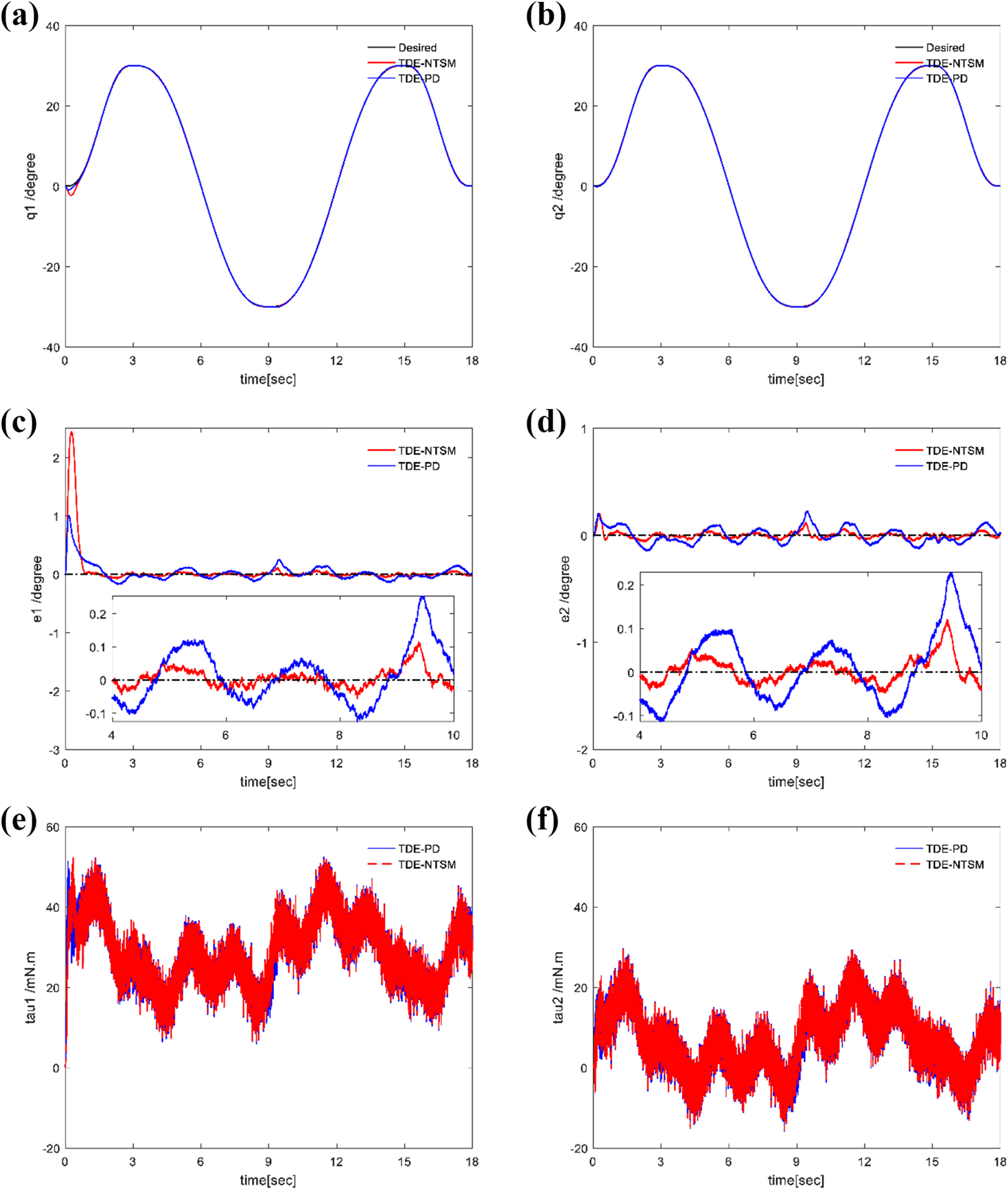
In the first case, to prove the control accuracy at different tracking speeds, the manipulator is required to run the same trajectory in different time. The periods are set to T = 12 s, 18 s, and 24 s, respectively. Corresponding simulation results are shown in Figures 6 to 8, meanwhile Tables 2 and 3 give the RMS and maximum values of control errors. In the following figures, the q _1,2 stand for position angles, e _1,2 represent the tacking errors, and tau_1,2 stand for τ _1,2 for joint 1 and 2, respectively.

Figure 6.

Case 1: T = 12 s. (a) and (b) show the comparisons between desired trajectory and actual trajectory of two controllers, (c) and (d) display the tracking error of both joints, and (e) and (f) show the control input of both joints.

Figure 7.

Case 1: T = 18 s. (a) and (b) show the comparisons between desired trajectory and actual trajectory of two controllers, (c) and (d) display the tracking error of both joints, and (e) and (f) show the control input of both joints.

Figure 8.

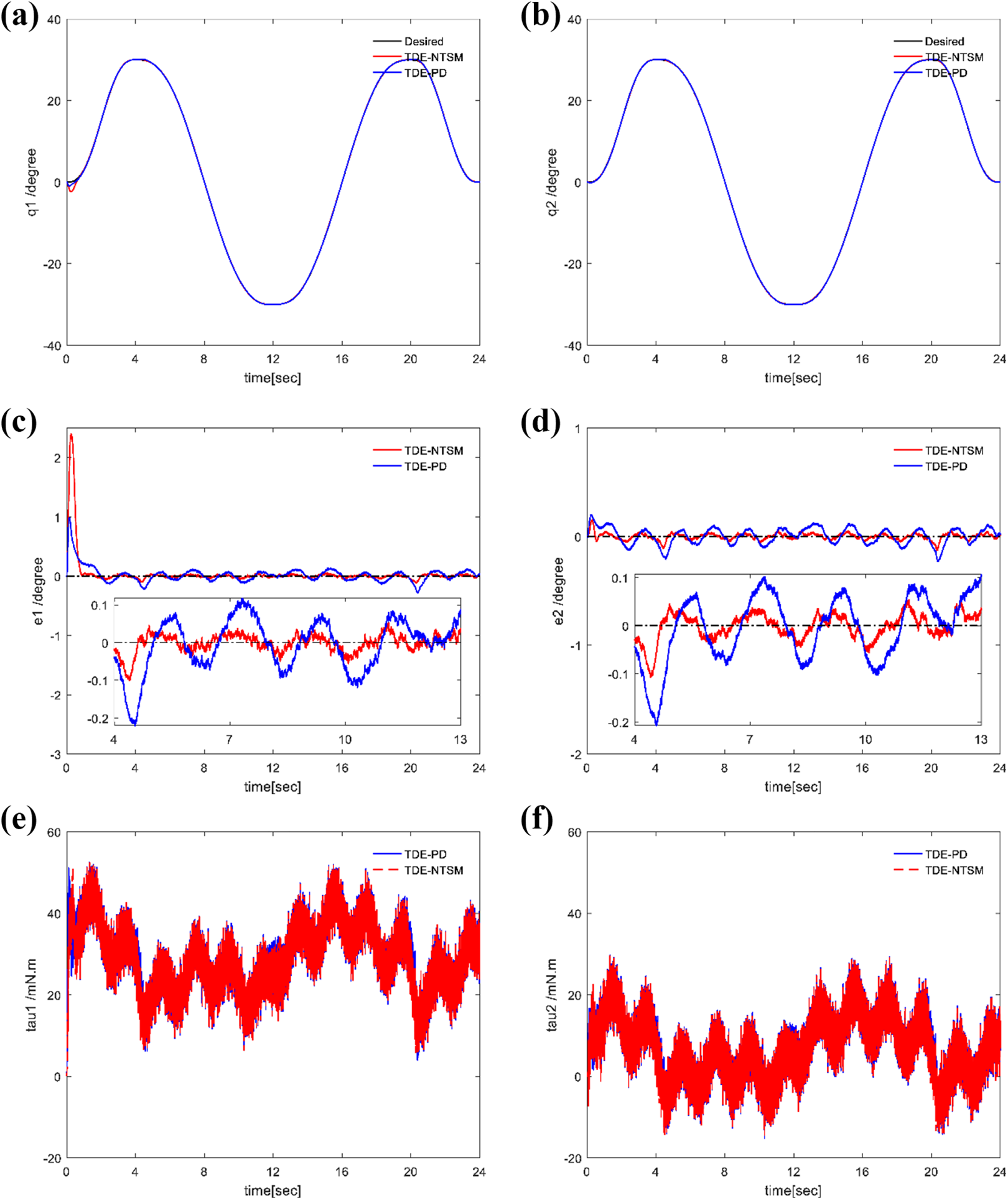
Case 1: T = 24 s. (a) and (b) show the comparisons between desired trajectory and actual trajectory of two controllers, (c) and (d) display the tracking error of both joints, and (e) and (f) show the control input of both joints.

Table 2.

RMS and maximum values of joint 1 control error.

(degree)	T = 12 s (RMS/Max)	T = 18 s (RMS/Max)	T = 24 s (RMS/Max)
TDE-NTSM	0.073/0.419	0.025/0.116	0.026/0.117
TDE-PD	0.109/0.376	0.074/0.253	0.074/0.281

RMS: root-mean square; NTSM: nonsingular terminal sliding mode, TDE: time-delay estimation.

Table 3.

RMS and maximum values of joint 2 control error.

(degree)	T = 12 s (RMS/Max)	T = 18 s (RMS/Max)	T = 24 s (RMS/Max)
TDE-NTSM	0.044/0.223	0.026/0.120	0.027/0.127
TDE-PD	0.084/0.285	0.068/0.228	0.070/0.226

RMS: root-mean square; NTSM: nonsingular terminal sliding mode, TDE: time-delay estimation.

As we can see from Figures 6 to 8, obviously, TDE-NTSM has a smaller control error than TDE-PD when control energies are almost the same at high and low speeds and with a decrease in tracking speed, the control precision is improving. We noted that in the simulation of T = 12 s, the control error has large peaks at some points, which is caused by the friction term in dynamic model when the manipulator reversing. We can see that the control error decreases which make those peaks become less apparent as simulation speed decreases. Furthermore, Tables 2 and 3 present that the RMS of TDE-NTSM is about 43% of TDE-PD’s, and the maximum value is about 50% smaller than that of the controller for comparison. Thus, we can draw a conclusion that the TDE-NTSM controller performs better.

Case 2: Sine and step

We added a step signal to the sinusoidal desired trajectory so as to demonstrate good robustness to external disturbances of the proposed controller, and the period is chosen as T = 18 s. Figure 9 gives the response results of two controllers to step signals and RMS and maximum value of control errors are presented in Table 4.

Figure 9.

Case 2. (a) and (b) show the comparisons between desired trajectory and actual trajectory of two controllers, (c) and (d) display the tracking error of both joints, and (e) and (f) show the control input of both joints.

Table 4.

RMS and maximum values of case 2.

(degree, T = 18 s)	Joint 1 (RMS/Max)	Joint 2 (RMS/Max)
TDE-NTSM	0.384/2.701	0.364/2.692
TDE-PD	0.450/2.649	0.445/2.638

As depicted in Figure 9, the step signal occurred in 4 s, 8 s, and 12 s. When tracking the sinusoidal trajectory, TDE-NTSM has a smaller error than TDE-PD. And in the face of step signal, TDE-NTSM can make error converge to a relatively small value in about 0.5 s while TDE-PD takes about 2 s. RMS and maximum values presented in Table 4 also validate the superiority of TDE-NTSM controller to external disturbances.

In this subsection, we simulated in two cases to demonstrate the effectiveness of the TDE-NTSM controller. The simulation results of the first case indicated that the proposed controller has better tracking performance than TDE-PD controller in both high speed and low speed. While in second case, step signal was added to the sinusoidal desired trajectory to detect the response of both controllers to sudden external disturbances. And the result showed that TDE-NTSM made error converge to the neighborhood of equilibriums in a shorter time.

Conclusion

In this article, we proposed a novel light cable-driven manipulator used for aerial autonomous operations. Thanks to the application of cable-driven technology, the drive unit of the manipulator can be installed at the base, which greatly simplifies the structure and reduces the quality of the moving part of the robot arm. Afterward, a TDE-NTSM controller was presented by combining the NTSM technique with TDE scheme. The NTSM control has the ability to generate high precision and fast convergence than the traditional PD control due to the utilization of a nonlinear SM surface. The nonlinear SM surface, that is, NTSM, can accelerate the convergence speed around the equilibrium point and therefore guarantee better comprehensive performance than the linear one or traditional PD control. Thanks to the utilization of NTSM technique, our developed TDE-NTSM controller can provide better control performance than the widely used TDE-PD controller. Simulation results show that the proposed controller has better control effect compared with the traditional TDE-PD controller.

Currently, we are trying to establish our first flying manipulator system using the designed light cable-driven manipulator given in this article. By removing the drive unit from the joints to base, our designed cable-driven manipulator can effectively reduce the moving inertia and energy consumption. Corresponding experimental results will be reported after we finish building the system. Meanwhile, the studies of control in task space and motion planning algorithms will also be performed after the system is established.

Footnotes

Declaration of conflicting interests

The author(s) declared no potential conflicts of interest with respect to the research, authorship, and/or publication of this article.

Funding

The author(s) disclosed receipt of the following financial support for the research, authorship, and/or publication of this article: This work was supported in part by the National Natural Science Foundation of China under Grant 51705243, in part by the Natural Science Foundation of Jiangsu Province under Grant BK20170789, in part by the China Postdoctoral Science Foundation under Grant 2019T120424 and in part by the Open Foundation of the State Key Laboratory of Fluid Power and Mechatronic Systems (GZKF-201915).

ORCID iD

Yaoyao Wang

Appendix 1

References

Gonçalves

Henriques

. UAV photogrammetry for topographic monitoring of coastal areas. ISPRS J Photogramm Remote Sens 2015; 104: 101–111.

Pirník

Hruboš

Nemec

, et al. Integration of inertial sensor data into control of the mobile platform. In: Proceedings of the 2015 federated conference on software development and object technologies, 2017, pp. 271–282. Berlin: Springer DOI: 10.1007/978-3-319-46535-7_21.

Pivarčiová

Božek

Turygin

, et al. Analysis of control and correction options of mobile robot trajectory by an inertial navigation system. Int J Adv Robot Syst 2018; 15(1): 1–15.

Amin

Shamshirband

. A review of quadrotor UAV: control methodologies and performance evaluation. Int J Autom Control 2016; 10(2): 87–103.

Ruggiero

Lippiello

Ollero

. Aerial manipulation: a literature review. IEEE Robot Autom Lett 2018; 3(3): 1957–1964.

Bai

. Digital twin-driven sustainable intelligent manufacturing: a review. Adv Manuf. DOI: 10.1007/s40436-020-00302-5.

Cao

, et al. Product sustainable design: a review from the environmental, economic, and social aspects. ASME J Comput Inf Sci Eng 2020; 20: 040801.

Cao

. Kinematics of underactuated robotics for product carbon footprint. J Clean Prod 2020; 257: 120491.

Zhu

Zhang

. Boundary encryption-based Monte Carlo learning method for workspace modeling. ASME J Comput Inf Sci Eng 2020; 20(3): 034502.

10.

Božek

Bezák

Nikitin

, et al. Increasing the production system productivity using inertial navigation. Manuf Technol 2015; 15(3): 74–278.

11.

Danko

. Design and control of a hyper-redundant manipulator for mobile manipulating unmanned aerial vehicles. J Intell Robot Syst 2014; 73: 709–723.

12.

Ramon

Arrue

Ollero

. Detection, location and grasping objects using a stereo sensor on UAV in outdoor environments. Sensors 2017; 17(12): 103–119.

13.

Ramon

Bevec

Arrue

, et al. Extracting objects for aerial manipulation on UAVs using low cost stereo sensors. Sensors 2016; 16(5): 700–716.

14.

Ollero

Heredia

Franchi

, et al. The AEROARMS project: aerial robots with advanced manipulation capabilities for inspection and maintenance. IEEE Robot Autom Mag 2018; 25(4): 12–23.

15.

Orsag

Korpela

. Modeling and control of MM-UAV: mobile manipulating unmanned aerial vehicle. J Intell Robot Syst 2013; 69: 227–240.

16.

Ikeda

Yasui

Minamiyama

, et al. Stable impact and contact force control by UAV for inspection of floor slab of bridge. Adv Robot 2018; 32(19): 1061–1076.

17.

Cafolla

Russo

Carbone

. Design of CUBE, a cable-driven device for upper and lower limb exercising. Mech Mach Sci 2019; 65: 255–263.

18.

Yuan

Chen

Yao

, et al. An improved online trajectory planner with stability-guaranteed critical test curve algorithm for generalized parametric constraints. IEEE/ASME Trans Mech 2018; 23(5): 2459–2469.

19.

Chen

Huang

Yang

, et al. Adaptive fuzzy backstepping control for stable nonlinear bilateral teleoperation manipulators with enhanced transparency performance. IEEE Trans Ind Electron 2020; 67(1): 746–756.

20.

Chen

Yao

, et al. Integrated coordinated/synchronized contouring control of a dual-linear-motor-driven gantry. IEEE Trans Ind Electron 2020; 67(5): 3944–3954.

21.

Cafolla

Russo

Carbone

. CUBE, a cable-driven device for limb rehabilitation. J Bionic Eng 2019; 16(3): 492–502.

22.

Abaunza

Castillo

Victorino

, et al. Dual quaternion modeling and control of a quad-rotor aerial manipulator. J Intell Robot Syst 2017; 88: 267–283.

23.

Božek

Al Akkad

Blištan

, et al. Navigation control and stability investigation of a mobile robot based on a hexacopter equipped with an integrated manipulator. Int J Adv Robot Syst 2017; 14(6): 1–13.

24.

Yuan

Chen

Yao

, et al. Fast and accurate motion tracking of a linear motor system under kinematic and dynamic constraints: an integrated planning and control approach. IEEE Trans Control Syst Technol 2019; 16: 1–8.

25.

Deng

Yao

. Extended-state-observer-based adaptive control of electro-hydraulic servo mechanisms without velocity measurement. IEEE/ASME Trans Mechatron 2019: 1–1 DOI: 10.1109/TMECH.2019.2959297.

26.

Deng

Yao

. Time-varying input delay compensation for nonlinear systems with additive disturbance: an output feedback approach. Int J Robust Nonlinear Control 2018; 28(1): 31–52.

27.

Jeong

Chang

Park

. Sensorless and modeless estimation of external force using time delay estimation: application to impedance control. J Mech Sci Technol 2011; 25(8): 2051–2059.

28.

Mendez-Monroy

Benitez-Perez

. Neuro-fuzzy control with time delay estimation for nonlinear networked control systems. Int J Innov Comput Inf Control 2011; 7: 4435–4450.

29.

Jin

Chang

, et al. High-accuracy tracking control of robot manipulators using time delay estimation and terminal sliding mode. Int J Adv Robot Syst 2011; 8(4): 65–78.

30.

Wang

Yan

Chen

, et al. A new adaptive time-delay control scheme for cable-driven manipulators. IEEE Trans Ind Inform 2019; 15(6): 3469–3481.

31.

Wang

, et al. Adaptive time-delay control for cable-driven manipulators with enhanced nonsingular fast terminal sliding mode. IEEE Trans Ind Electron. 2020: 1–1 DOI: 10.1109/TIE.2020.2975473.

32.

Wang

Liu

Wang

, et al. Time-delay control using a novel nonlinear adaptive law for accurate trajectory tracking of cable-driven robots. IEEE Trans Ind Inform 2020; 16(8): 5234–5243.

33.

Wang

Yan

Zhu

, et al. A new practical robust control of cable-driven manipulators using time-delay estimation. Int J Robust Nonlinear Control 2019; 29(11): 3405–3425.

34.

Ait

Schönlein

Jordan

. Estimation of linear positive systems with unknown time-varying delays. Eur J Control 2013; 19(3): 179–187.

35.

Cho

Jin

Kuc

, et al. Control and synchronization of chaos systems using time-delay estimation and supervising switching control. Nonlinear Dyn 2014; 75(3): 549–560.

36.

Liu

. Neural adaptive sliding mode speed tracking control of a DC motor. J Syst Eng Electron 2004; 15(3): 304–318.

37.

Bazzi

Chalhoub

. Fuzzy sliding mode controller for a flexible single-link robotic manipulator. Modal Anal 2016; 11(2): 295–314.

38.

Niu

Lam

. Robust integral sliding mode control for uncertain stochastic systems with time-varying delay. Automatica 2005; 41(5): 873–880.

39.

Karray

Feki

. Adaptive and sliding mode control of a mobile manipulator actuated by DC motors. Int J Autom Control 2014; 8(2): 173–190.

40.

Wang

Zhu

Chen

, et al. Model-free continuous nonsingular fast terminal sliding mode control for cable-driven manipulators. ISA Trans 2020; 98: 483–495.

41.

Guo

Yan

. Globally finite-time stable three-dimensional trajectory-tracking control of underactuated UUVs. Ocean Eng 2019; 189: 106–122.

42.

Feng

Man

. Non-singular terminal sliding mode control of rigid manipulators. Automatica 2002; 38(12): 2159–2167.

43.

Wang

Yan

, et al. Practical adaptive fractional-order nonsingular terminal sliding mode control for a cable-driven manipulator. Int J Robust Nonlinear Control 2018; 29(5): 1396–1417.

44.

Pourhashemi

Ramezani

Siahi

. Designing dynamic fractional terminal sliding mode controller for a class of nonlinear system with uncertainties. Int J Autom Control 2019; 13(2): 197–225.

45.

Wang

, et al. Practical tracking control of robot manipulators with continuous fractional-order nonsingular terminal sliding mode. IEEE Trans Ind Electron 2016; 63(10): 6194–6204.

46.

Bensaada

Boudghene

. A practical design sliding mode controller for DC–DC converter based on control parameters optimization using assigned poles associate to genetic algorithm. Int J Electr Power Energy Syst 2013; 53: 761–773.

47.

Sun

. Discrete-time fractional order terminal sliding mode tracking control for linear motor. IEEE Trans Ind Electron 2018; 65(4): 3386–3394.

48.

Ramirez-Rodriguez

Parra-Vega

Sanchez-Orta

, et al. Robust backstepping control based on integral sliding modes for tracking of quadrotors. J Intell Robot Syst 2014; 73: 51–66.

49.

Chang

, et al. Particle swarm optimization tuned fuzzy terminal sliding mode control for UPS inverters. J Intell Fuzzy Syst 2015; 29(6): 2483–2488.

50.

Mobayen

Tchier

, et al. Design of an adaptive tracker for n-link rigid robotic manipulators based on super-twisting global nonlinear sliding mode control. Int J Syst Sci 2017; 48(9): 1990–2002.

51.

Wang

Chen

Yan

, et al. Adaptive super-twisting fractional-order nonsingular terminal sliding mode control of cable-driven manipulators. ISA Trans 2019; 86: 163–180.

52.

Wang

Zhu

Yan

, et al. Adaptive super-twisting nonsingular fast terminal sliding mode control for cable-driven manipulators using time-delay estimation. Adv Eng Softw 2019; 128: 113–124.

53.

Gadoue

Giaouris

Finch

. MRAS sensorless vector control of an induction motor using new sliding-mode and fuzzy-logic adaptation mechanisms. IEEE Trans Energy Convers 2010; 25(2): 394–402.

54.

Lee

Tsai

. The structural synthesis of tendon-driven manipulators having a pseudotriangular structure matrix. Int J Robot Res 1991; 10(3): 255–262.

55.

Sang

Wang

, et al. Control design and implementation of a novel master-slave surgery robot system, MicroHand A. Int J Med Robot Comput Assist Surg 2011; 7: 334–347.

56.

Jin

Lee

Tsagarakis

. Model-free robust adaptive control of humanoid robots with flexible joints. IEEE Trans Ind Electron 2017; 64(2): 1706–1715.

57.

Shirinzadeh

, et al. Continuous finite-time control for robotic manipulators with terminal sliding mode. Automatica 2005; 41(11): 1957–1964.

58.

Lee

Chang

. Control of a heavy-duty robotic excavator using time delay control with integral sliding surface. Control Eng Pract 2002; 10(7): 697–711.

59.

Wang

Liu

Chen

, et al. Practical robust control of cable-driven robots with feedforward compensation. Adv Eng Softw 2020; 145: 102801.

A light cable-driven manipulator developed for aerial robots: Structure design and control research

Abstract

Keywords

Introduction

Structure design

Coupling analysis

Controller design and simulation studies

Controller design

Comparisons with existing TDE-PD controller

Simulation setup

Simulation results

Case 1: With different speeds

Case 2: Sine and step

Conclusion

Footnotes

Declaration of conflicting interests

Funding

ORCID iD

Appendix 1

References