
Abstract
Inverse kinematic equations allow the determination of the joint angles necessary for the robotic manipulator to place a tool into a predefined position. Determining this equation is vital but a complex work. In this article, an artificial neural network, more specifically, a feed-forward type, multilayer perceptron (MLP), is trained, so that it could be used to calculate the inverse kinematics for a robotic manipulator. First, direct kinematics of a robotic manipulator are determined using Denavit–Hartenberg method and a dataset of 15,000 points is generated using the calculated homogenous transformation matrices. Following that, multiple MLPs are trained with 10,240 different hyperparameter combinations to find the best. Each trained MLP is evaluated using the R 2 and mean absolute error metrics and the architectures of the MLPs that achieved the best results are presented. Results show a successful regression for the first five joints (percentage error being less than 0.1%) but a comparatively poor regression for the final joint due to the configuration of the robotic manipulator.
Keywords
Introduction
Determining kinematic properties of a robotic manipulator is a crucial step in any work relating to the use of the robotic manipulator. Before any further calculations can be performed, direct and inverse kinematic equations need to be determined. Direct kinematic equations allow the transformation from the joint variable space into the tool configuration space, that is, calculation of the position of tool in workspace from predefined joint rotation values. 1 Inverse kinematic equations allow the opposite transformation from the tool configuration space to the joint variable space, that is, if we know the position in the workspace that we are trying to achieve, we can calculate the joint values necessary to position the tool at that location. While the determination of the robotic manipulator direct kinematics is relatively straightforward, and there are methods such as Denavit–Hartenberg (D-H) that allow for the simple determination, determining inverse kinematics is a more complex process. 2 Determining the inverse kinematic equations for complex robots has high algebraic complexity. 3 Determining the solution numerically is an option, but it takes a comparatively long time compared to using a direct solution, such as an equation.
In this article, a method is proposed in which multilayer perceptron (MLP) is used to regress the equations for the inverse kinematic equations for each joint. ANN is an artificial intelligence or machine learning algorithm 4 that can be used for solving various regression and classification tasks. 5,6 Artificial intelligence methods such as this have a wide variety of applications. ANNs and other artificial intelligence methods, such as evolutionary computing algorithms, 7 –9 have a wide variety of uses in robotics in areas such as computer vision 10,11 and path optimization 12 –14 and navigation. 15,16 ANN emulates the human neural system using a structure of nodes, referred to as neurons, that are interconnected with weighted connections. 17,18 By adjusting this weight depending on the data, ANNs can provide the ability to classify or regress the input data to a solution with high precision. 18,19 Robotic manipulator used is modeled after a realistic six degrees of freedom (6-DOF) manipulator ABB IRB 120.
State-of-the-art
Villegas et al. 20 use the dataset adaptation technique to solve the inverse kinematic issue, by ANN retraining using data points with higher error values. This approach shows promising results in rising the accuracy of the trained ANN. Nemeth et al. 21 show the use of machine learning methods, such as classification trees and clustering, in the process of detecting failures in production systems. The authors show a successful detection of failures using these methods, using data collected from control program’s logged files. Ghafil et al. 22 attempt to solve inverse kinematics of 3-DOF robotic manipulator using Levenber–Marquardt, Bayesian regularization, and scaled conjugate gradient learning algorithms. Results show that the best results are provided when using the Bayesian regularization algorithm. Demby et al. 23 show the use of a reinforcement learning method, specifically ANNs and adaptive neurofuzzy inference systems. While their methods show some ability to regress, the authors conclude that the results are not accurate enough for use. Ghasemi et al. 24 show the use of an ANN for the determination of inverse kinematics on a simple 3-DOF RRL robotic manipulator. The proposed solution shows that ANNs have the ability to be used for kinematic determination for a simpler robotic manipulator. Dash et al. 25 attempt to regress the inverse kinematic equations using the ANN. The authors conclude that the results achieved are not satisfactory, as they have a very low accuracy especially for the second and sixth joint of the manipulator, most probably caused due to a low number of training data and no hyperparameter variation. Zarrin et al. 26 show the application of the ANN for the direct control of a soft robotic system. This article shows a successful application of the ANN in use with robotic manipulators. Takatani et al. 27 use a neural network to achieve determination of joint values. The authors propose the use of a complex, multi-ANN model to learn the inverse kinematics without the use of evaluation functions. The results show that, for a 3-DOF, robotic manipulator solution like the proposed one can provide satisfactory results. Dereli and Köker 28 propose a metaheuristic artificial intelligence solution for inverse kinematic calculation. Multiple algorithms are compared by authors (quantum behaved particle swarm, firefly algorithm, particle swarm optimization, and artificial bee colony) and best results are shown when using quantum behaved particle swarm. Lim and Lee 29 discuss the number of points necessary for the inverse kinematic solutions. Their findings show that regression can be learned with as little as 125 experimentally obtained data points.
Hypotheses
This article is trying to prove three hypotheses and these are as follows: a MLP ANN can be used to determine inverse kinematics of a realistic 6-DOF manipulator instead of a more complicated method, determine the best possible configuration of the MLP for determining inverse kinematics of each joint, and a dataset virtually generated from direct kinematics can be used for ANN training.
The novelty of this article is twofold. First, it lays in the fact that an artificially generated dataset has been used to train the neural network. Using an artificially generated dataset, training of inverse kinematics networks for a new robotic manipulator can be performed significantly faster than when an experimental dataset is used (provided that the results are satisfactory). This would allow for training of the neural networks in such a case where the robotic manipulator is not readily available to the researchers to perform a large number of experimental measurements upon. The second part lays in the fact that only the x, y, and z spatial positions of the end effector are used as inputs without the orientations of the end effector. In case that satisfactory result can be achieved this way, the method would show the ability to regress the inverse kinematics problem without the need for measurement of the Euler angles, which define the orientation, simplifying training of such neural networks.
In continuation, first, the methodology will be presented. The method used for determining direct kinematics and the dataset generation will be explained. After that, a description of MLP ANNs is given, along with the methods for hyperparameter determination and solution quality estimation. Finally, results are presented and discussed along with the drawn conclusions.
Methodology
In this article, the methodology used in our research will be presented. First, the process of determining the direct kinematic equations of the robotic manipulator will be described, followed by the description of a way those equations were used to generate a used dataset. The overview of the ANN will be given, along with the description of chosen activation functions and hyperparameters used during the grid search process. Finally, the way authors evaluated the quality of the obtained solutions will be presented.
Direct kinematic equation determination
Direct kinematic equations are determined using the D-H algorithm. In the D-H algorithm, each joint is assigned a sequential number i from 1 to n, where 1 depicts the first joint of the robotic manipulator nearest to the base and n depicts the last joint of the robotic manipulator.
30
Then, the recursive D-H algorithm is started. In the first iterative part, each joint is assigned a right orthonormal coordinate system Lk
, where
dk
: translation along axis
xk
: translation along axis
For a rotational joint,
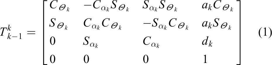
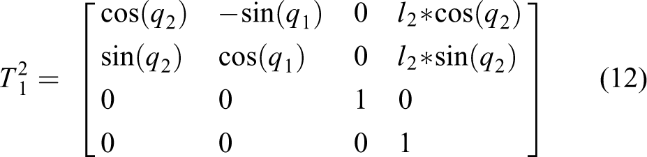
Because of the size of the equations, the shortened trigonometric format is used. When using this format, the trigonometric functions are written using only the first letter of their name, so sine is written as S and cosine as C. In addition, the arguments of the functions are written as indexes. The kinematics matrix for the entire robotic manipulator, connecting the base of the robotic manipulator and the tool, is calculated as a product of the homogenous transformation matrices

in which
r
1 is the perpendicular vector,
r
2 is the movement vector, and
r
3 is the approach vector.
Robotic manipulator tool positioning can be defined using

with x, y, and z being robotic manipulator end-effector positions in the tool configuration space, and

and

where
Dataset generation
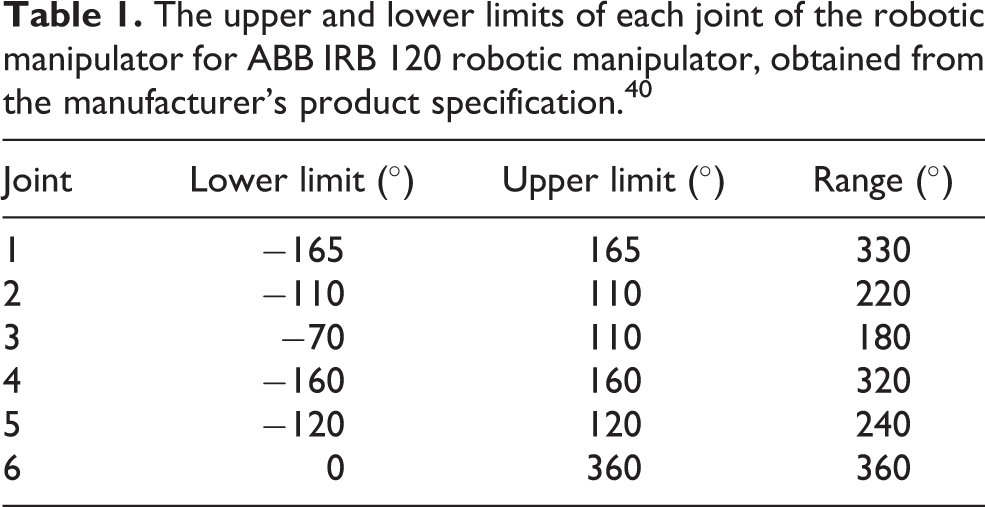
To generate the dataset, first, the possible joint values need to be defined. Figure 1 shows the robotic manipulator in diametric view with joint axes displayed. The limits of joint angle values for each joint are given in Table 1. On the figure, axes 1 through 6 represent the rotational axis of the corresponding joint of the robotic manipulator, with the arrows representing the directions in which the given joint is capable of rotating.
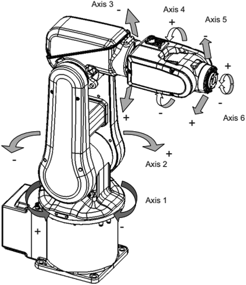
Diametric view of the robotic manipulator with axes displayed 40 (Axes 1–6: Rotational axes of the robotic manipulator).
The upper and lower limits of each joint of the robotic manipulator for ABB IRB 120 robotic manipulator, obtained from the manufacturer’s product specification. 4 0
A random value is generated for each joint within its given range. These values are generated with a uniform random distribution. Then, the direct kinematic equations are used to calculate the x, y, and z coordinates of the robotic manipulator end effector. Doing this yields a dataset of 15,000 data points, which is a large enough amount to attempt a regression analysis using artificial intelligence techniques. 29 Furthermore, analysis of the values in the dataset shows that all of the input and output values are unique, allowing for unique mapping from the inputs to outputs. While this dataset could have been generated experimentally, through robot positioning and measurement of joint angles, this would have taken an extremely long time and would have added the problem of measurement imprecision and errors. Generating dataset in the manner described in this article was chosen by the authors because of the wish to test the possibility of using an artificially generated dataset for ANN training.
Multilayer perceptron regressor
MLP is a type of a feed-forward ANN, consisting of an input layer, output layer, and at least one hidden layer, 41 consisting of one or more artificial neurons. 42 The value of each neuron starting with inputs is propagated to the neurons in the next layer over connections. Each connection has a certain weight, which signifies the importance of the value of that neuron to the value of the neuron it is connected to. The sum of values of all neurons of the previous layer connected to the current neuron is then transformed using the activation function of the neuron in question and the new value of that neuron is calculated. 43 The value of the input neurons is weighted, summed, and transformed over each neuron in the first hidden layer, and this is repeated for each following layer until the final, output, layer is reached and the values of neurons are weighted and summed giving the output value. 44,45
From the above, it can be seen that the weights of the connections play an important part in value determined as the output. Because of this property, it is important to set connection weights as accurately as possible, which is done in the training stage during which the data stored in the dataset are used to adjust the connection weights. 43,45
Each of the inputs xi
has a corresponding weight

where X is the vector of inputs described in equation (7) and
The output value of the neurons is calculated as

where
The error of the neural network is propagated back through the network (meaning, in the direction from the output neuron to the input neurons), with the goal of adjusting the connection weights.
49,50
Gradients are used to allow the adjustment of values depending on their difference from the goal value, where error

where α represents the learning rate of the ANN
52,53
and m is a total number of data points. The higher this rate is, the faster the weights
In addition to value of neurons, there is another value taken into account in each layer. This value is referred to as bias and marked with bi . Bias is the value that allows the adjustment of the origin point of the activation function. 43,57 This enables neural networks to be adjusted in a way that allows solving problems, which have the solutions near the origin point of the coordinate system of the solution space. 58 –60
Hyperparameter determination
In the previous sections, a number of values have been mentioned, such as learning rate α, hidden layers, and the number of neurons in each as well as the activation functions. These values are parameters that describe the neural network itself, or more precisely, its architecture. To differentiate these parameters from parameters contained within the neural network, namely the values of weights
Values of hyperparameters determine how well the ANN will perform the task it was designed to. The hyperparameters of the neural network varied in this article are hidden layers (number of layers and neurons per each layer 63 ), activation function of the neurons, solver, initial learning rate, type of learning rate adjustment, and regularization parameter L2. 51,64,65 The values of hyperparameters used in the research are given in Table 2.
Possible values for each hyperparameter used in grid search for determining the best ANN architecture.a

a First column gives hyperparameter values of which are defined in the second column. Third column provides a total number of possible parameter values. For the “hidden layers” row, each tuple represents an ANN setup, where each hidden layer is represented by an integer equaling the number of neurons it contains. 66
The total number of combinations, that is, ANN architectures, can be calculated as a product of numbers of possible values for each hyperparameter, which means that the total of ANN architectures tested is 10,240.
The hyperparameters are tested using the grid search method. 67 In grid search method, the combination of each of the above parameters is given, and a neural network with those hyperparameters is calculated. 68,69 Additionally, each combination of parameters is executed 10 times due to the cross-validation process described in the following section.
Solution quality estimation
After the training using the parameters obtained using an iteration of grid search, the other part of the dataset is used as the testing set. In testing, the trained MLP attempts to determine the value of the set inputs, which are compared to the real outputs. The difference between this process and training is that no adjustment is done in this part—there is no backpropagation, just the forward. This enables the quality of the neural network to be determined, as the values it predicts are compared to the values that have not been used in training and as such did not have an effect on the trained weights of the neural network. Once the predicted set
Two values are used to determine the quality of the solution: coefficient of determination (R 2) and mean absolute error (MAE).
The coefficient of determination is defined as the proportion of variance in the dependent variable predictable from the independent variables.
70,71
This provides information on how much of the variance in the data is explained by the predicted data.
72,73
Let vector
With these two values, the coefficient of determination R 2 is defined by 76 –78

MAE is defined as 79
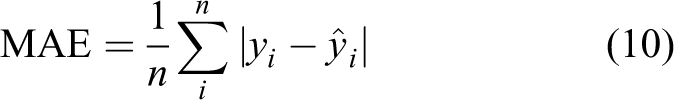
and it provides the information of what is the average difference between real values in vector y and corresponding predicted values in vector
R
2 is defined in range
To assure the stability of the ANN models across various sets of data, cross validation has been applied. Tenfold cross validation has been used. This process splits the dataset into 10 parts (folds) randomly. Then, the training is repeated 10 times. In each of these iterations, one of these folds is used as a testing set, while the other nine are used as a training set. This allows for the entirety of the dataset to be used for testing, determining the quality of the achieved solution across the entirety of the dataset.
Results
This section represents the results obtained by the authors during the research. First, the kinematic parameters and direct kinematic equations obtained are presented, followed by the results obtained from ANN training.
Direct kinematic properties
Performing D-H method on the ABB IRB 120 robotic manipulator yields the schematic shown in Figure 2. On the schematic, each joint of the robotic manipulator is represented with a dotted circle. L
0 through L
5 represent the origins of coordinate system of each joint, while

Simplified schematic of the modeled robotic manipulator with coordinate systems determined using D-H method (Dotted circle: manipulator joint; L0–L6: coordinate system origins; x0–x6, y0–y6, z0–z6: coordinate system axes; b1–b6: x and z axes intersection points). D-H: Denavit–Hartenberg.
For the observed robotic manipulator, the values of kinematic parameters are presented in Table 3. By inserting values from Table 3 into the homogenous transformation, matrices of each joint using equation (1) matrices shown in equations (24) to (29) are obtained.
Kinematic parameters of the robotic manipulator determined using the D-H method.


and

Multiplication of this matrix per equation (2) yields the homogenous transformation matrix of the robotic manipulator as follows

where

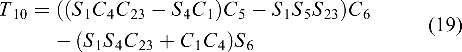


and

Equations (31) to (46) represent each of the elements of the matrix
Multilayer perceptron regression
The results for the most successful models for each joint are selected. As mentioned, models R 2 and MAE performance metrics on the training set are observed as the determination of quality. The results are given in Table 5. Where possible, a simpler architecture with comparable results was chosen due to a simpler architecture having better training times. Shorter training times are apparent in the simpler neural networks (where simpler means a lower number of neurons) due to the lower number of connection gradients and weights that need to be calculated during the backpropagation stage in training. The ratio of MAE and the total range for the joint as given in Table 1 are also presented in Table 4.
Percentage error for each joint in regards to its maximum movement range.

MAE: mean absolute error.
The best architecture found during the grid search process.a

MAE: mean absolute error.
a For each joint best hyperparameters and achieved performance metrics are given.
Discussion
The obtained results demonstrate a successful regression of the inverse kinematics problem. All the solutions achieve the MAE, which is smaller than 1% of the possible joint angle range. Only model which has an error larger than 1° or 0.1% of the joint angle range is the q 6. The larger error of the q 6 can be explained by the fact that the dataset does not contain the tool orientation data, which has a large influence on the joint in question. From Figures 1 and 2, it can be seen that joint 6 is the final torsion joint of the robotic manipulator, meaning its direct influence is not exhibited on the X, Y, and Z positioning of the end-effector position. R 2 scores achieved by the networks are above 0.9 in all cases except for the q 6 output, which can be explained in the same manner as the high MAE for the regressed angle value of the sixth joint. Except for the q 6, the worst performing network in terms of R 2 score is the regressor for the third joint q 3, with R 2 score of 0.9. Still, even with a comparatively low R 2 score, it achieves a low MAE of 0.04°. Except for the q 6, in terms of the MAE, the worst performing regression model is q 4, with MAE of 0.12°, still a relatively high R 2 score is displayed (0.94) by the regression model in question. Standard errors across the 10 folds of the algorithms are low for both metrics used, indicating stable solutions for all the regression goals.
Observing the hyperparameters, it can be seen that the number of the hidden layers and neurons per layer tend toward the higher end of the tested hyperparameters. Four of the best performing networks (for the regression goals
Conclusion
This article presents the application of MLP ANN for the goal of inverse kinematics modeling. Grid search algorithm has been applied and the best hyperparameters for each of the six output goals have been determined. The scores achieved are satisfactory, with all models achieving an error below 1% of the appropriate output range. The models of the first five joints tended toward the largest tested networks. This indicates that higher quality results, if such are needed, may possibly be achieved with even larger networks. The last joint having a lower regression score indicates a lack of information, due to it only being affected by the orientation of the end-effector data, which was not used in the dataset. This implies that modeling of similarly configured robotic manipulators using the described method may require that data if a high precision is needed for the final joint.
Future work will include the testing of other methods, which may yield simpler to use models, such as symbolic regression, and the expansion of the dataset include obstacle data.
Footnotes
Declaration of conflicting interests
The author(s) declared no potential conflicts of interest with respect to the research, authorship, and/or publication of this article.
Funding
The author(s) disclosed the receipt of following financial support for the research, authorship, and/or publication of this article: This research was (partly) supported by the CEEPUS network CIII-HR-0108, European Regional Development Fund under the grant KK.01.1.1.01.0009 (DATACROSS), project CEKOM under the grant KK.01.2.2.03.0004, CEI project “COVIDAi” (305.6019-20), University of Rijeka scientific grant uniri-tehnic-18-275-1447 and the project VEGA 1/0504/17.