
Abstract
The problem of optimal tracking control for robot–environment interaction is studied in this article. The environment is regarded as a linear system and an admittance control with iterative linear quadratic regulator method is obtained to guarantee the compliant behaviour. Meanwhile, an adaptive dynamic programming-based controller is proposed. Under adaptive dynamic programming frame, the critic network is performed with radial basis function neural network to approximate the optimal cost, and the neural network weight updating law is incorporated with an additional stabilizing term to eliminate the requirement for the initial admissible control. The stability of the system is proved by Lyapunov theorem. The simulation results demonstrate the effectiveness of the proposed control scheme.
Keywords
Introduction
Robot applications are becoming more and more widespread, such as rehabilitation therapy, assembly automation and surgery. 1 –4 They can either work independently to accomplish tasks or cooperate with their human partners for certain tasks. In the actual application process, the robot will inevitably interact with the external environments. 5 –7 Consequently, in recent years, interaction control between the robot and environment has attracted great concern and is considered to be greatly important.
In existing research, two main approaches are applied to achieve compliant behaviour of the robot, that is, hybrid position/force control and impedance control. 8,9 The first approach requires the position subspace and force subspace decomposition, task planning and control law switching in the execution process. Without considering the dynamic coupling of the environment and the robot, the accuracy of the hybrid position/force control cannot be guaranteed. 10 In contrast, the second approach aims to adjust the mechanical impedance to a target one, which will guarantee the robot to be complaint with the interaction force imposed by the external environment. Impedance control ensures the safety of the robot and the environment and it has been proved to be more feasible and has better robustness. According to the causality of the controller, impedance control has two implementation methods, one is named impedance control and the other is admittance control. In impedance control system, the interaction force can be estimated from the desired motion trajectory and impedance model, while in admittance control system, the reference trajectory is obtained from the measured environmental external force and the desired admittance model. Therefore, in this article, admittance control is adopted to solve the problem of robot–environment interaction control.
In admittance control system, force and the admittance model are two important parts. When robot–environment interaction exists, the force can be detected and measured by the sensors installed on the end-effector of the robot arm. But, how to derive optimal parameters of the admittance model is non-trivial. On the one hand, it is usually difficult to derive the desired admittance model because of the complexity of environmental dynamics; on the other hand, a fixed admittance model cannot satisfy all cases. Taking human–robot cooperation as an example, variable admittance control is necessary to ensure more efficient performance. 11 To solve these problems, iterative learning has been studied in robot intelligent control area. It has been investigated to obtain admittance parameters to adapt to unknown environment. The aim of this approach is to introduce human learning skills into the robot and improve control performance by repeating a task. Cohen and Flash 12 proposed an impedance learning control scheme using an associative search network to complete a wall-following work. Neural network (NN) is introduced into the impedance control to regulate the parameters. 13 However, the iterative learning method requires the robot to operate repeatedly, which brings inconvenience in practical process and is not feasible in many situations. Love and Book, 14 Uemura and Kawamura, 15 Gribovskaya et al., 16 Stanisic and Fernández, 17 Landi et al. 18 and Yao et al. 19 have proposed to utilize adaptation approaches to address the problems stated above.
Robotic motion control is a challenging task as it is difficult to obtain accurate model concerning that the robot is a non-linear and highly coupled system. Proportional–integral–derivative (PID) control, NN control, adaptive control and other control methods have been applied to the robot system. 20 –27 As a classical control method, PID control is employed to the robot system and can track the given reference trajectory well. 28 It is acknowledged that PID control has some advantages, such as simple structure and good robustness, but it is not easy to select suitable PID parameters if the controlled plant is complex. In addition, when dynamic uncertainties exist in the system, PID control cannot satisfy the performance requirements for the magnitude of overshoot, the rising and settling time and so on. NN has the fundamental characteristics of human brain and can simulate human behaviour for information processing, therefore it is widely used in the control field for unknown system identification. NN control can model the uncertain dynamics online to improve the system performance. 29 An admittance adaptation method and the NN-based controller are applied into the robot system. 30
Tracking control is a significant research issue in the domain of robot intelligent control. For a controlled system, stability is just the minimum requirement. Optimal control needs to be considered, that is, it is required to design an optimal tracking controller, which could ensure system stability of the robot while minimizing the cost function. Werbos 31 proposed adaptive dynamic programming (ADP) strategy and it is considered to be an effective approach to resolve the optimal control problem. 32 The key of ADP method is to find a solution of Hamilton–Jacobi–Bellman (HJB) equation. However, because it is a partial differential equation, when the controlled system is non-linear but not linear, its analytical solution will be very difficult to obtain, or even impossible. To solve the above problem, policy iterative is considered as an effective method to find the approximate solution, which requires initial stability control. 33 However, in practical process, the initial admissible control is usually very difficult to satisfy. Then, NN is introduced to derive an approximate solution of the HJB equation. The approximate solution is obtained by NN-based method, meanwhile the requirement of initial stability is eliminated with the incorporation of an additional term. 34,35
Yang et al.
30
paid attention to the robot–environment interaction control, but did not consider the optimization problem. However, for the robot, how to perform path tracking optimization and minimize the cost function is very important. Based on the above discussion, the optimal tracking control problem for robot–environment interaction is studied in this article. Moreover, the admittance control and ADP approach are adopted to improve the system performance. The contributions of this article are listed below: The environment with unknown dynamics is modelled as a linear system. An admittance adaptation method with iterative linear–quadratic regulator (LQR) is obtained to achieve a compliant behaviour. ADP approach is introduced into the robot system to solve the optimal tracking problem. The critic network with radial basis function (RBF) is developed to approximate the minimum cost function. In addition, to eliminate the requirement for initial admissible control, a stabilizing term is incorporated into NN weight updating law.
The rest of this article is arranged as follows. Firstly, the robot and environment systems and control objectives are described. Next, the control scheme including admittance adaptation and optimal control using ADP is developed. Then, simulation studies are given. Finally, the conclusion is drawn.
Preliminaries and problem formulation
Robot dynamics
The n-link robot manipulator dynamics is showed as the following Lagrangian form

where
Define the reference trajectory as

Then, the first and second time derivative of qe are given below

We define the sliding motion surface ξ as follows

where

Substituting equation (5) into equation (1), the error dynamics is obtained as follows

Then, the following system is obtained

The non-linear functions

Environment dynamics
It is assumed that the dynamics of environmental interaction force subject to the equation given below

where CE and GE represent the unknown damping and stiffness of the environment, respectively. F denotes the interaction force and can be detected and measured by a force sensor. x is the end-effector position in Cartesian space and the corresponding desired trajectory xd is defined as

where

If we take equation (11) as a linear system with F as its control input and η as its states to be controlled, this equation relates x with xd
via the optimal feedback control law
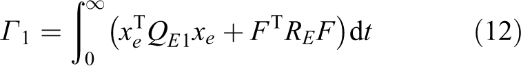
This cost function also indicates that our motivation of modifying a desired trajectory xd
is to balance the contact force F with the tracking error
In this section, the robot and environment dynamics are modelled. Then, we will design a control strategy to achieve the compliant behaviour and optimal tracking control in case the robot interacts with the environment.
Control scheme
A control scheme consisting of three parts as shown in Figure 1 including an optimal trajectory modifier using admittance control, a closed-loop inverse kinematics (CLIK) solver and a trajectory tracking controller based on ADP technique is designed in this section.

An illustration of the proposed control scheme.
Trajectory modification using admittance control
The solution to equation (12) is an analogy with the LQR problem. It can be rewritten as

whose system counterpart is consistent with equation (11).
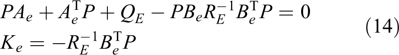
In this subsection, an algorithm proposed by Jiang and Jiang 36 is adopted to solve the algebraic Riccati equation (ARE) in equation (14) with unknown environment parameters CE , GE to derive the feedback gain Ke
Some notations are outlined here. n, m and d are the length of η, F and the sample times integer, respectively. The sampled signal together with the historical ones comprising the matrix as follows

where

When the number of sampled data is large enough and the rank condition in equation (16) is satisfied, the algorithm can solve Ke
by iteratively calculating equation (17) until

where the superscript
Once the optimal feedback gain Ke is obtained, we can use it to modify xd . Formulations are given as below

where

Inverse kinematics using CLIK
The CLIK algorithm is employed to resolve the Cartesian reference trajectory xr
into the one qr
in joint space.
37
Let the solution error

where Kf
is a positive user-defined matrix that decides the convergent rate of e. Expanding the above equations and combining with

integrating of which yields the CLIK method

where
Optimal control using ADP
As mentioned in the Introduction section, it is very important to optimize the trajectory tracking while minimizing the design cost for robots. On the basis of optimal theory, the optimal control of the system (7) can be derived by solving the HJB equation in the frame of ADP. Consequently, in this subsection, our target is to find such an optimal control μ.
Assume that the functions
where

where
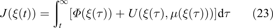
Then, the Hamiltonian function and the optimal cost function of robot system (7) are defined as below


We can obtain the HJB equation shown as

Suppose that the minimum value on the right side of formula (27) exists and also is unique, from

Substituting the optimal control law (28) into equation (24) yields another form of HJB equation with respect to

Inspired by Liu et al.,
34
we know that if the optimal function

where

From equations (28) and (31), the following

Then, substituting equations (31) and (32) into equation (29), we have

where


In fact, the ideal weight w and

Then, the derivative of equation (36) is

Based on equations (28) and (37), the approximate optimal control is obtained as

Similarly, applying equations (25), (37) and (38), the approximate Hamiltonian function

Define eH
as the error between


According to equations (33), (39) and (41), eH in equation (40) can be described as

To train RBFNN, an appropriate weight updating law


where
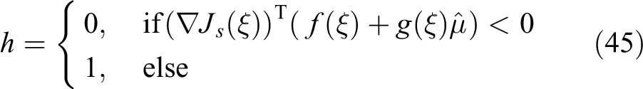
where

It should be noted that
Stability analysis
In this subsection, we will analyse the stability of the system and give the detailed proof that the approximate error
Theorem 1
Consider the robot system (7) with approximate optimal control (38) and the NN weight updating law (43), then it is concluded that the approximate error
Proof
See the Appendix.
Numerical simulation
Simulation settings
A two-degree-of-freedom (2-DOF) planar manipulator is adopted to verify the proposed control scheme. It is constructed by the robotics toolbox with parameters shown in Table 1.
38
The numerical simulation shown in Figure 2 runs on the MATLAB 2018a software where an ode3 solver is chosen with a fixed time step of 0.01 s, simulation time 20 s and other settings remain default. The initial joint position is

where CE
, GE
and x
0 are chosen as
Parameters of the robot manipulator.


Settings of the numerical simulation.
For the proposed control scheme, parameters are set as below: to calculate the optimal trajectory in equation (13),
Simulation results
In this subsection, two cases will be compared to demonstrate the validity of the proposed scheme. Note that, the environment dynamics of the simulation is not totally consistent with that in equation (9), and x
0 is unknown. Therefore, two different Ke
values are considered and examined. Case 1: the feedback gain
Simulation results are shown in Figures 3 to 6. Figure 3 shows the modification process of the user-defined trajectory along the x-axis of both cases. It is not until around 4.1 s that the rank condition in equation (16) is satisfied following that the trajectory starts being modified. During the transient process, it can be found that the modified trajectory of Case 2 has a slight oscillation, and this subsequently triggers larger tracking errors compared with Case 1. The steady state and force pair of Case 1 and Case 2 trajectories at 10.28 s are 0.13 m/−0.07 N and 0.14 m/−0.06 N, respectively, which is in line with the time series of the cost function in equation (12) of both cases as shown in Figure 4. From the figure, we can see that after the modification of trajectory, the cost function of Case 1 is smaller than that of Case 2, which implies that in this simulation settings where the actual existence of unknown x 0 cannot be neglected, the feedback gain obtained from the proposed scheme is more appropriate. Note that, due to the unknown x 0, the environment dynamics in equation (9) used for the designing of the trajectory modifier differentiates from that in equation (47) used for simulation. Therefore, under this situation, actually neither the Ke of Case 1 nor Case 2 is the optimal one. However, the proposed method still works and regards the dynamics in equation (47) as a linear one with an appropriate feedback gain. This has demonstrated the effectiveness of the proposed admittance control method.

Simulation results of trajectory modification. (a) Case 1,

The time series of cost function in equation (12),

Modified trajectories corresponding to the different choice of

Simulation results of control performance. (a) Case 1,
Figures 5
to 7 are plotted for analysing the performance of the ADP-based controller. Figure 6 shows the control torques τ and sliding mode surface z of Case 1 and Case 2. On the whole, the proposed scheme tracks the both modified trajectory well, given that only nine neurons are used in the RBFNN, and the control torques are within the physical limitation. Besides, weights convergence can be observed in Figure 7. Note that, because of the introduced additional term
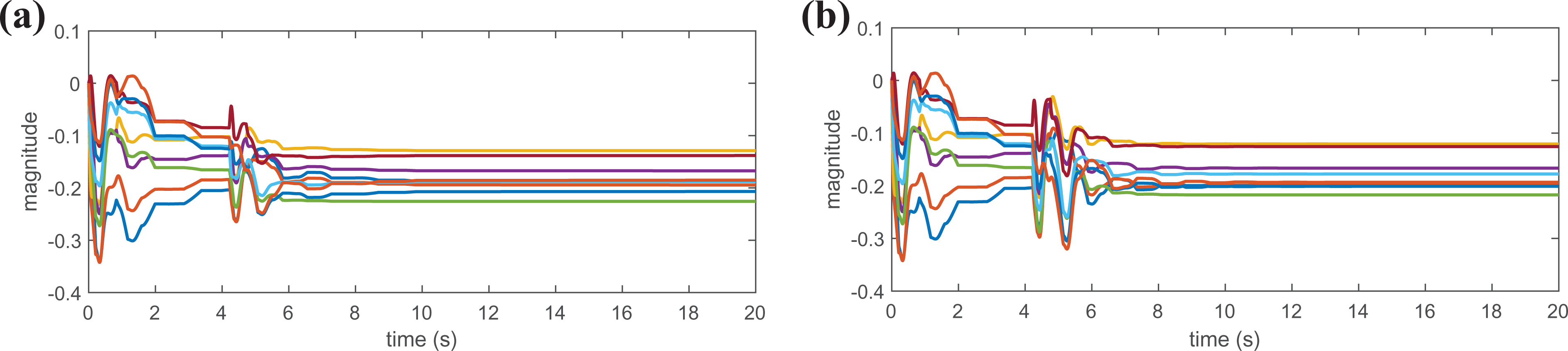
Weights of the RBFNN. (a) Case 1,
Feedback gains of different

Conclusion
The optimal control of robots interacting between unknown environment was studied in this article. An ADP-based controller with admittance adaptation was proposed. The unknown environment was regarded as a linear system and a compliant behaviour was guaranteed by the admittance adaptation control. In addition, NN was introduced into ADP controller to ensure trajectory tracking of the robot with minimal cost. The stability of the robot system was proved and simulation studies demonstrated the effectiveness of the proposed control scheme.
Because of the complexity of the robot system, dynamic uncertainties and input constraints such as saturation and dead zone are very common in robot systems, which will not only affect system performance but also may lead to system instability. 24,39,40 Therefore, in the frame of ADP, the optimal control problem with dynamic uncertainties and input constraints will be considered in our future work.
Footnotes
Declaration of conflicting interests
The author(s) declared no potential conflicts of interest with respect to the research, authorship, and/or publication of this article.
Funding
The author(s) disclosed receipt of the following financial support for the research, authorship, and/or publication of this article: This work was partially supported by Engineering and Physical Sciences Research Council (EPSRC) under grant EP/S001913 and Shenzhen Science and Technology Plan Project [JSGG20180507183020876].