Sage Journals: Discover world-class research

Abstract

In the field of visual perception, the edges of images tend to be rich in effective visual stimuli, which contribute to the neural network’s understanding of various scenes. Image smoothing is an image processing method used to highlight the wide area, low-frequency components, main part of the image or to suppress image noise and high-frequency interference components, which could make the image’s brightness smooth and gradual, reduce the abrupt gradient, and improve the image quality. At present, there are still problems such as easy blurring of the edges of the image, poor overall smoothing effect, obvious step effect, and lack of robustness to noise on image smoothing. Based on the convolutional neural network, this article proposes a method for edge detection and deep learning for image smoothing. The results show that the research method proposed in this article solves the problem of edge detection and information capture better, significantly improves the edge effect, and protects the effectiveness of edge information. At the same time, it reduces the signal-to-noise ratio of the smoothed image and greatly improves the effect of image smoothing.

Keywords

Convolutional neural network image smoothing deep learning edge detection

Introduction

The image has rich and well-structured visual information, but it is often disturbed by noise during transmission and acquisition. Edge smoothing of images helps guide the computer to more accurately recover images, analyze and extract visual information in images more efficiently, and facilitate more advanced visual tasks. Therefore, it is particularly important to study the image edge smoothing as an image processing technology in the field of image processing.

Image smoothing helps to eliminate various interference noises, so that the high-frequency components in the image fade and the contrast reduced, save the low-frequency components, and the image information is extracted and saved most efficiently for subsequent processing of the image. This article is based on the application of convolutional neural network (CNN) and edge detection in image smoothing; deep learning of image processing is carried out by edge information detection and network feature fusion. The results show that the CNN proposed in this article solves the problem of edge detection and information capture better in image smoothing research, significantly improves the edge effect, makes the edge features more prominent, and protects the effectiveness of edge information. Anti-noise ability makes the image smoothing effect more natural.

The first section illustrates the relevant difficulties of this topic and introduces the subject matter of this article; the second section summarizes the research content of the current relevant literature; the third section includes a detailed description of the test methods used in this article; the fourth section is the experiment part containing the description of the experimental data and experimental steps; the fifth section presents the experimental results, and the analysis of the experimental results; and the sixth section summarizes the results of this article.

Related work

At present, there are many research studies on image smoothing methods. The content of image smoothing is mainly two aspects: one is the elimination of image detail texture and noise, and the other is to enhance or protect the edge features of the image. Foreign research on image smoothing started earlier and achieved fruitful results.¹ Nhat-Duc et al.² established and compared two intelligent methods to automatically identify the performance of pavement cracks. The experimental results show that the CNN-based model has good prediction performance (classification accuracy rate (CAR) = 92.08%), which is better than the edge detection algorithm-based method (CAR = 79.99%). Yahya et al.³ proposed a new image edge detection technique based on a combination of total variation and anisotropic diffusion models. The superiority of the new method in eliminating false edges and improving edge positioning accuracy is proved. Shahdoosti and Rahemi⁴ trained the network by using edge maps obtained from the well-known Canny algorithm, the purpose of which is to determine if the noise patches in the non-subsampled Slicelet domain correspond to the position of the edges. The results show that this method has better performance than some of the latest noise reduction methods. Choi et al.⁵ suggested a three-dimensional (3D) block-based residual encoder decoder convolutional neural network (REDCNN) model that uses a convolutional layer paired with a deconvolution layer, a shortcut, and a residual map to preserve the image structure and diagnostic features of the image and improve image resolution by smoothing noise. The method was found to effectively reduce the Poisson noise level without losing diagnostic function and exhibit high performance in both qualitative and quantitative evaluations. Cai et al.⁶ used the image processing of intelligent buildings as the basic theoretical platform, and based on the pattern recognition technology, studied image processing, image extraction, and image recognition in image processing of building intelligent environment, and proposed reasonable solutions. De Silva et al.⁷ proposed and evaluated two wavelet-based edge feature enhancement methods to pre-process the input image by CNN, developed a new pre-processing layer, and attached it to the network architecture. The results show that the proposed method is superior to the baseline and previously published work. Dhar et al.⁸ detected license plates from car images, detects pre-processing of input images, edge detection, morphological extension and filtering region properties, and verifies the shape of the plate by using a reliable boundary distance (DtBs) method and by using the CNN performs automatic feature extraction to identify the extracted characters. Simulation results show that the accuracy is very low. Wen et al.⁹ introduced a novel dark-guided coarse-to-fine CNN framework to solve the super-resolution problem. Under the guidance of color information, the depth of the obtained high-resolution image can alleviate texture copy artifacts and effectively preserve edge details.

In the past, the research on smoothing algorithms has been deepened, and various smoothing algorithms based on different concepts have been proposed. However, its central idea is nothing more than the setting of weights. These weights are basically linear, and the application of multi-feature fusion networks and deep learning in information extraction and prediction are ignored in these algorithms. Some algorithms use statistical ideas to achieve image smoothing. Such algorithms can reduce image blur and preserve image edge information more effectively, but the biggest disadvantage is that the algorithm is quite time-consuming. These all determine that the various algorithms above are not optimal image smoothing algorithms.

CNNs are a class of feedforward neural networks with convolutional computation and deep structure. They are one of the representative algorithms of deep learning. Deep learning is a branch of machine learning. Since CNNs are capable of translation-invariant classification, they are also referred to as “translation-invariant artificial neural networks.” With the introduction of deep learning theory and the improvement of numerical computing equipment, CNNs have developed rapidly. The CNN constructs the visual perception mechanism of the creature, which can be supervised and unsupervised. The convolution kernel parameter sharing and the sparseness of the interlayer connection in the hidden layer make the CNN smaller. Volume-to-grid features, such as pixel and audio learning, have a stable effect and have no additional feature engineering requirements for the data; therefore, it is widely used in the fields of image recognition, object recognition, behavioral cognition, pose estimation, and neural style conversion. Li Feiteng¹⁰ found that the convolutional neural network hidden markov model (CNN-HMM) hybrid model has higher accuracy in vocabulary recognition than the deep neural network hidden markov model (DNN-HMM) hybrid model. CNN and DNN contain a large number of matrix operations in the process of optimizing the learning parameters. In large-scale image and speech recognition, this process becomes very slow. Using NVIDIA GPU to accelerate matrix operations can achieve dozens of times and hundreds of times performance improvement over CPU. Chang Liang and Deng Xiaoming¹¹ described the basic theory of CNNs and elaborated on the specific aspects of image understanding, such as image classification and object detection, face recognition and semantic segmentation of scenes. Hongtao and Qinchuan¹² summarized the basic model structure, convolution feature extraction, and pooling operation of CNNs, and summarized the CNN model based on deep learning in image classification, object detection, attitude estimation, image segmentation, and face recognition. Li et al.¹³ introduced the deep recursive convolutional network (DRCN) interpolation algorithm into the interpolation of polarization camera, and gave the degree of linear polarization (DoLP) and polarization angle of DRCN single image. The DRCN algorithm is compared with bicubic interpolation, and the interpolation error of the algorithm is smaller than the error of bicubic interpolation. Using the DoFP polarization camera with two different resolutions to shoot the same scene, the DoLP calculated with DRCN interpolation is closer to the real DoLP than the DoLP calculated with bicubic algorithm. Guo et al.¹⁴ used the CNN in deep learning to reduce the dependence on rich experience when designing feature extraction algorithms. The research shows that the CNN has a good performance in the license plate classification, and the recognition rate is as high as 98.25%. It also proves that deep learning has great application prospects in the field of intelligent transportation.

Method

Edge detection and edge information processing

Edge detection operator

The edge detection operator is the most basic method for edge detection. It can check the neighborhood of each pixel and quantify the gray rate of change, usually including the direction. There are several methods that can be used, most of which are based on a directional derivative mask for convolution. The general edge detection operators include Sobel edge operator, Roberts edge operator, Kirsch edge operator, and Prewitt edge operator. These operators can achieve better results when applied to images with a certain gray scale, but the effect is not ideal in color images. Although the RGB color space is often used to explain the basic principles of color formation, it is often used for the input and output operations of digital images because it does not conform to human visual perception, and is not suitable for edge detection, image segmentation, and so on that rely more on visual perception operation.

Therefore, we propose to use the HIS color space system as the space system mainly used for edge detection. “H” is the chromaticity, indicating the type of color, which is an important parameter for the reaction color change, and is also the main criterion for edge detection. A large amount of edge information is obtained by contrast of chromaticity. Since “H” becomes unstable at the low intensity and low saturation, the edge information is deviated. Therefore, it is necessary to normalize the chromaticity contrast, which means assigning corresponding coefficients according to saturation and intensity.

Linear fuzzy membership function

The “low” of low saturation and low intensity is relative to the overall pixel, that is, if sorted in ascending order, the pixels in front are considered to be low saturation (μ_s ) and low intensity (μ_j ). The specific approach is selecting a large linear fuzzy membership function based on trapezoidal distribution. The general form is as follows

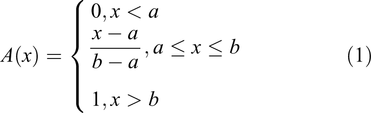
A (x) = \{\begin{cases} 0, x < a \\ \frac{x - a}{b - a}, a \leq x \leq b \\ 1, x > b \end{cases}

In the application here, A(x) is μ_s or μ_j , and x is the corresponding “s” value or “j” value, wherein a = 0 is a threshold. Usually set as follows (take the saturation s as an example): sort the M × N pixel saturation values from small to large, and then select $\frac{M \times N}{5}$ pixels as the threshold, which is “b.” That is to say, the pixel saturation value ranked in the first 20% is regarded as low saturation, and the pixel fuzzy membership function value is uniformly quantized to 1, which is regarded as non-low saturation. The function diagram of the fuzzy function is shown in Figure 1.

Figure 1.

Linear fuzzy function.

Low-intensity threshold selection is similar to saturation, but usually selected $\frac{M \times N}{5}$ pixels as the threshold. That is, the pixel intensity value ranked in the top 20% is considered to be low intensity. The large-scale linear fuzzy membership function based on trapezoidal distribution is easy to understand and has certain operability. However, due to the simple structure of such fuzzy membership functions, the practicality is fine when the fuzzy set is small. When a large image with more than 10,000 pixels is encountered, when the fuzzy set is large, the positioning of such linear fuzzy membership functions is less accurate. Therefore, corresponding to color image processing, we need to set a nonlinear fuzzy membership function to quantize the fuzzy concept.

Combination of RGB and HSI edge information

Such edge information is difficult to detect when the chromaticity is similar and the saturation and intensity are different. Therefore, we need to use other color space systems as a means to assist in detecting edge information. Since the color space system is the basic space system of color images, it has become the main auxiliary means. By calculating the contrast of the pixel information, the defect of obtaining the edge information by a single use chromaticity can be compensated to some extent. Based on the image pixel contrast definition, we use the Minkowski distance to calculate the contrast of the pixel information and take a value of 1. Therefore, its contrast formula is

{Contrast}_{RGB} = {[{(R_{1} - R_{2})}^{4} + {(G_{1} - G_{2})}^{4} + {(B_{1} - B_{2})}^{4}]}^{1 / 4}

Thus, the weighted average contrast obtained in combination with the normalized chromaticity contrast obtained according to the above formula is as follows

{Contrast}_{e g} = \frac{n_{1} {Contrast}_{1.2 HSI} + n_{2} {Contrast}_{1.2 RGB}}{n_{1} + n_{2}}

where n ₁ and n ₂ are the weights of the HSI and RGB spaces. According to the proportion of the two in obtaining edge information, take n ₁ = 0.2 and n ₂ = 0.4, respectively. So far, the work of acquiring pixel integrated edge information has been completed. The next work is to obtain the corresponding edge information in the four directions of the edge and compare it with the set threshold to determine whether it is an edge.

Positioning of edge properties

After determining the method of obtaining the edge information, we need to locate the edge, non-edge, or blur edge of the edge property of each pixel. First we need to determine the direction of the edge. We can divide the edges into four directions: vertical, horizontal, left diagonal, and right diagonal, as shown in Figure 2.

Figure 2.

Four edge extension directions obtained from the position of adjacent pixel blocks.

The horizontal double arrow in the figure determines the edge direction 1, the vertical double arrow determines the edge direction 2, the left oblique double arrow determines the edge direction 3, and the right oblique double arrow determines the edge direction 4. The edge information in each direction is obtained by two adjacent pixel blocks in the corresponding direction of the pixel, respectively. Specific steps are as follows:

According to ${\bar{C}}_{i j, b} = \frac{\sum_{q = s}^{s + 3} \sum_{p = r}^{r + 3} n_{p q} \cdot C_{p q}}{\sum_{q = s}^{s + 3} \sum_{p = r}^{r + 3} n_{p q}}$ calculating weighted average H, S, and I values of two adjacent pixel blocks in each edge direction of the pixel, where C is a corresponding H, S, and I value.

The average weighted average of the two pixel blocks is S, I, and the values are averaged to obtain the CI _s value and CI _j value in the corresponding edge direction.

According to ${Contrast}_{1.2 HSI} = {Contrast}_{1.2HSI} \times μ_{s} \times μ_{i}$ (H normalization formula), respectively calculate the normalized chromaticity H contrast in the corresponding edge direction.

According to equations (2) and (3), the contrasts ultimately used to locate the edge properties in the respective edge directions are calculated.

After completing the above steps, we obtain the edge information of the integrated HSI space and RGB space in the four edge directions. By taking its maximum value and comparing it to the set edge threshold, we can locate the corresponding edge properties. Both the edge threshold and the gray threshold are used to determine the nature of the pixel correlation. The difference is that because we need to determine the fuzzy edges, we need to set two large and small edge thresholds, namely “τ_h ” and “τ_j. ” When locating the edge properties, there are three cases:

Contrast _eg max > τ_h , positioning the pixel as an edge,

Contrast _eg max < τ_j , positioning the pixel to be non-edge, and

τ_j < Contrast _eg max < τ_h , positioning the pixel as a blurred edge,

where τ_h is the same as the conventional threshold τ_sm used in color image smoothing; τ_j = τ_h /10.

Since the edge image is generally a binary image, after the edge and the non-edge are positioned, the gray values of the pixels are defined as 1 and 0, 1 is an edge pixel, and 0 is a non-edge pixel. As a result, most of the edges have been processed.

Image smoothing method based on CNN

Deep convolution network structure

The deep convolutional network structure frame can be divided into three layers, namely an input layer, an implicit layer, and a pooling layer. The input layer of a CNN can process multidimensional data.^15,16 Typically, the input layer of a 1D CNN receives a 1D or 2D array, where a 1D array is typically time or spectrally sampled. A 2D array may contain multiple channels. An input layer of a 2D CNN receives a 2D or 3D array and an input layer of a 3D CNN receives a 4D array. The standardization of input features is beneficial to improve the operating efficiency and learning performance of the algorithm. The hidden layer of the CNN includes three common constructions: convolutional layer, pooled layer, and fully connected layer. In some modern algorithms, there may be complex structures such as inception module and residual block. In common construction, the convolutional layer and the pooled layer are unique to CNNs. The order in which the three types are commonly constructed in the hidden layer is usually: input-convolution layer-pooling layer-convolution layer-pooling layer-fully connected layer-output. The upstream of the output layer in the CNN is usually a fully connected layer, so its structure and working principle are the same as those in the traditional feedforward neural network.

Training process

The training set of this article is selected from the ILSVRC 2013 ImageNet data set, which includes 395,909 regular natural scene images and biological images. It is also the largest image data set in the world and can provide rich training data for deep CNN training. The calculation steps are as follows:

Define variables and parameter initialization.

The input image x is divided into sub-block images that do not overlap, and the sub-block image size is f _sub × f _sub. If the input image length is less than an integer multiple of f _sub, the sub-block image is internally expanded.

After inputting the sub-block image of f _sub × f _sub into the first layer network, convolution filtering is performed on the sub-block image by using a filter of size f ₁ × f ₁.

Feeding the output of the first layer to the second layer, and performing convolution filtering on the second layer with a filter of f ₂ × f ₂ size.

Feeding the output of the second layer to the third layer, and performing convolution filtering on the third layer with the filter of the f ₃ × f ₃ size on the third layer.

The output of the third layer is “y,” using the error evaluation criterion to estimate the distortion of the network input and output, and whether the evaluation error is minimum, if yes, jump to step (8); if not, continue to step (7).

Using filter weight update criteria, updating the weight of each layer of the filter, jump to step (3).

End training.

Edge detection method based on CNN

Through deep learning training, it will have better feature representation ability and enhance the understanding ability of image targets. In this article, based on ImageNet training, the parameters of deep convolutional network model are obtained, and the feature extraction and representation ability of the network is fully utilized to detect the edge of the image target. The algorithm calculation steps are as follows:

Define variable and parameter initialization: image size is M × N, input image is x, output image is y, input image sub-block length is f _sub, first layer filter length is f ₁, and second layer filter length is f ₂. The third layer filter has a length of f ₃.

Graying the input image x.

Dividing the gray image into nonoverlapping sub-block images, the sub-block image size is f _sub × f _sub, and if the input image length is less than an integer multiple of f _sub, the sub-block image is internally expanded.

After inputting the sub-block image of f _sub × f _sub into the first layer network, convolution filtering is performed on the sub-block image by using a filter of size f ₁ × f ₁, and the filter parameter is a value obtained by training.

The output of the first layer is directly sent to the third layer, and the output image of the second layer is convoluted and filtered by the filter of f ₃ × f ₃ size on the third layer, and the filter parameter is the value obtained by the training.

Performing binarization processing on the output image y.

End edge detection.

Image smoothing optimization solution

The forward calculation and error backward propagation of the CNN can complete part of the learning task, while the supervised optimization process and the use of the gradient to generate the weight increment are performed by the solver. The solver can optimize the model, and its evaluation index is to make the loss function reach the global minimum. Different algorithms have better solution effects under certain conditions, the most commonly used stochastic gradient descent (SGD) solver. The end point of the solver is the global optimization problem that minimizes the loss function. For data set D, the optimization goal is to lose the function mean over the full data set D

L (W) = \frac{1}{|D|} \sum_{i}^{|D|} f_{w} (X_{i}) + λ r (W)

where f _w(X_i ) is the loss function on the data instance X_i , r(W) is the regular term, and λ is the weight of the regular term. For the image data used in the network training process of this article, there are tens of thousands of windows per iteration, using the batch gradient descent method, and each iteration uses only the random approximation of this objective function, taking N data instances

L (W) = \frac{1}{|N|} \sum_{i}^{|N|} f_{w} {(X}_{i}) + λ r (W)

According to the principle of batch gradient descent and hardware performance, the batch size takes N = 256 in the subsequent training process. When the training set, similar samples are repeated, the processing method converges faster. The example is as follows: Assume that in the training set training process, the first half of the data and the second half of the data have the same gradient, then if the first half of the data is a batch and the latter half is another batch, then in the traversal of the data set, the overall method is only one step ahead, and the processing method advances two steps to the optimal solution of training. There are more training data in this article, and it is slower to traverse the entire data set. The method of processing reduces the computational pressure of the processor and converges to the optimal solution more quickly.

In the forward propagation process, the model calculates the loss function f_w , and in the backward propagation process, calculates the gradient f_w Δ. The weight increment ΔW is obtained by the solver through the error gradient f_w Δ, the normalized gradient Δr(W), and other method-related terms. The SGD method updates the weight W using a linear combination of the negative gradient ΔL(W) and the weight update history V_t . The learning rate α is the weight of the negative gradient, and the forgetting factor μ is the weight of the weight update history V_t . Knowing V_t ₊₁ and weight W_t of the V_t iteration, V_t ₊₁ and W_t ₊₁ of the $t + 1$ th iteration can be calculated by the following formula

\begin{array}{l} V_{t + 1} = μ V_{t} - α Δ (W_{t}) \\ W_{t + 1} = W_{t} + V_{t + 1} \end{array}

The hyperparameters of the learning process also need to be adjusted, and the initial learning rate α and the forgetting factor μ will be set by empirical values.

Experiments

Experimental conditions

This article runs the software environment 64-bit WIN7 operating system, using Microsoft Visual Studio 2013 as a compilation tool, the simulation tool is Matlab 2014b software, and the deep learning tool is NVIDIA GPU toolkit CUDA and CUDNN. CUDA and CUDNN are parallel computing tools developed by NVIDIA for the deep learning network working on the GPU, the experimental condition and configuration are listed in Table 1. The Caffe package provided by Northwestern University is a deep learning network tool library that includes the relevant library functions needed to build a deep learning network.

According to the filter size design method in the classical deep convolution network,¹⁷ the first layer is 9 × 9 size filter, that is, f ₁ = 9; the second layer is 1 × 1 size filter, that is, f ₂ = 1; the third layer is 5 × 5 size filter, that is, f ₃ = 5.

Table 1.

Experimental condition and configuration.

Software environment	Parameter configuration
Operating system	WIN7 64-bit
Compilation tool	VS 2013
Tool library	Caffe
Simulation tool	Matlab 2014
GPU toolkit	CUDA 7.0, CUDNN

Experiment process

Experimental evaluation criteria

The experimental process of this study is shown in Figure 3, which include edge information detection, deep learning algorithm, pixel processing, contrast, saturation optimization, and the edge determine, and so on.

Figure 3.

Experiment process.

(1) Average accuracy

Comparing the performance of each classifier on the same test set often requires reference to some key performance indicators. For example: F-score, precision-recall curve, false positive per image (FPPI), miss rate curve, receiver operating characteristic (ROC) curve, and area under curve (AUC). Taking into account the accepted evaluation criteria of the actual test data set and the distribution of positive and negative samples, this article uses the precision (research)-recall (review) curve as the evaluation index, and uses the average precision (AveP) to measure the overall credibility of the classifier. To describe the precision-recall curve, the description of the two-class confusion matrix is shown in Table 2.

Table 2.

Description of the two-class confusion matrix.

	Sample prediction			Statistics
		Negative	Positive	Statistics
Actual sample	Positive	FN	TP	FN + TP
Actual sample	Negative	TN	FP	TN + FP
Statistics		TN + FN	TP + FP

TP: correctly affirm the number of samples; FN: missing the number of samples; FP: number of false positive samples; TN: correct negative sample number.

In the precision-recall curve evaluation index, precision = TP/(TP+FP) indicates the probability that the prediction is correct in the positive sample, and recall = TP/(TP+FN) indicates the probability that the prediction is correct in the actual positive sample.¹⁸ The more the precision-recall curve of a classifier in the plane rectangular coordinate system is convex to the upper right, indicating that the performance of this classifier is better. In addition, since the precision-recall curve is affected by the test sample, there will be a large fluctuation of the curve, so the AveP is generally used to measure the performance of the classifier. The concept of AveP is to divide the detection result of a series of data q into N parts according to the recall rate. The average detection accuracy AveP of the series of data is

AveP (q) = \frac{\sum_{recall = 1 / n}^{1} precision}{N}

The average accuracy of multiple series of data means the mean of the AveP of each series of data, which can be used to evaluate the comprehensive performance of the algorithm in multiple types of targets. Its expression is

m AP = \frac{\sum_{q - 1}^{Q} AveP (q)}{Q}

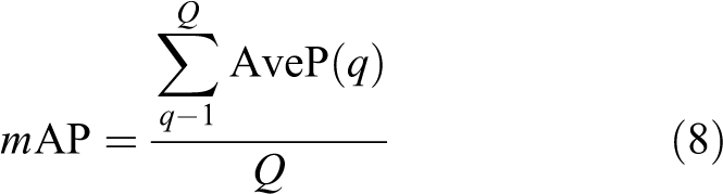
where Q is the total number of series of data.

(2) Overlap

The degree of overlap is the degree of coincidence between the detection result and the target frame of the human calibration. Different overlap degree reflects the credibility of the algorithm, and high overlap also represents higher requirements for positioning accuracy. Its expression is

Overlap = \frac{B_{j} \cap b_{m j}}{B_{j} + b_{m j} - B_{j} \cap b_{m j}}

where B_j is the algorithm detection frame, b_mj is the calibration detection frame, and $B_{j} \cap b_{m j}$ represents the intersection of the two detection frames.

(3) Average frame rate

The frame rate is the number of frames displayed per second. The average frame rate is the total number of frames divided by the total number of seconds when the algorithm detects the target for a period of time. The average frame rate reflects the computational complexity of the detection algorithm and is the basis for measuring the real-time performance of the detection algorithm.

Results and discussion

Edge information extraction

The edge detection effect diagram is shown in Figure 4. The algorithm proposed in this article mainly detects the edge of the contour of the object, which can basically reflect the contour features of the image content, and there is no more scene edge information. It effectively improves the accuracy of edge information extraction.

Figure 4.

Comparison of pre-process and post-process images.

By comparison, it is found that the algorithm proposed in this article can only deal with the information concentration area better, and can effectively maintain the characteristics, thus improving the detection efficiency. The figure reflects the information concentration area of the original image. In comparison of the figure, the edge image obtained by the algorithm is obviously more accurate than the edge image obtained based on the linear fuzzy membership function, and the edge is more delicate. This is because at the edge of the color image, mostly the low saturation and low intensity gathering regions, the resulting standardized chromaticity H contrast can better reflect the edge information of the original image.^19,20 In addition, in the area included in the edge of the object, the case where the non-edge pixel is mistakenly judged as the edge pixel is also reduced. The above is the main experimental result of the algorithm. Edge images obtained using only the RGB color space and edge images obtained using only the HSI color space are listed separately. Edge information cannot be accurately extracted using only RGB or HSI. Non-edge pixels are mistakenly judged as edge pixels, and HSI is the opposite. Thus, it is necessary to combine the two to get the edge of the image more effectively. This is a supplementary explanation in the experimental results.

Signal-to-noise ratio analysis

In order to further analyze the effectiveness of the edge detection method based on the deep convolution network and compare it with the Canny algorithm, this study uses the signal-to-noise ratio as the evaluation index to measure the edge detection efficiency. The signal-to-noise ratio (SNR) is

SNR = S_{edge} / N_{noise}

where $S_{edge}$ is the number of signal edges and $N_{noise}$ is the number of noise edges.

The image effect before and after denoising is shown in Figure 5, and the signal-to-noise ratio of the edge detection results is shown in Table 3. According to the results of Table 3, it can be found that the algorithm proposed in this article is more obvious than the Canny detection algorithm. This is because the algorithm proposed in this article can understand the target object through deep convolutional network learning of large-scale data. The edge processing is concentrated on the target object, and the edge of the nontarget object is less detected.

Figure 5.

Image effects before and after denoising. The picture on the left is before denoising and the picture on the right is after denoising.

Table 3.

Signal-to-noise ratio obtained by different algorithms after processing.

Image name	Signal-to-noise ratio
Image name	Proposed algorithm	Canny algorithm
Baboon	1.33	1.51
Barbara	2.00	1.21
Bridge	1.12	1.15
Coast	3.01	1.04
Comic	1.11	1.18
Face	1.71	1.00
Flowers	1.81	1.88
Foreman	2.31	1.29
Lenna	2.14	1.78
Man	2.55	1.45
Monkey	2.54	1.36
Pepper	1.88	1.59
Rabbit	1.99	1.21
Zebra	2.81	1.01
Average	2.02	1.33

According to Table 3, it can be found that the Canny algorithm has a higher signal-to-noise ratio for images with only a target or a single scene.²¹ The reason is that the detection performance of the deep convolution network depends on the training of the training set. The network can learn various scenarios and analyze the target from the scene.²² Therefore, the application of the algorithm requires a large amount of network training to achieve a better smoothing effect.

Image smoothing effect after deep learning

The CNN uses the BP framework for learning in supervised learning. Through multiple deep learning, the image smoothing algorithm based on CNN is optimized. The pooling layer has no parameter update in back propagation, so it is only necessary to assign the error to the appropriate position of the feature map according to the pooling method. For the maximal pooling, all errors will be assigned to the position of the maximum value; pooling, the error is evenly distributed across the pooled area.

The results in Figure 6 show that the effect of shape detail can be enhanced based on the algorithm proposed in this article, but for the image with strong contrast, the result is flatter than the original image, which weakens the stereoscopic effect and realism to some extent, so the improvement introduces some parameters. Control global and local comparisons, make necessary additions and enhancements to the edge information contained in a single input image to obtain the best balance point for better processing results. The local histogram also reflects the pixel distribution information of the image, which is consistent with the general histogram. It can be seen from Figure 7 that the processed image pixel distribution is effective.

Figure 6.

Image smoothing effect.

Figure 7.

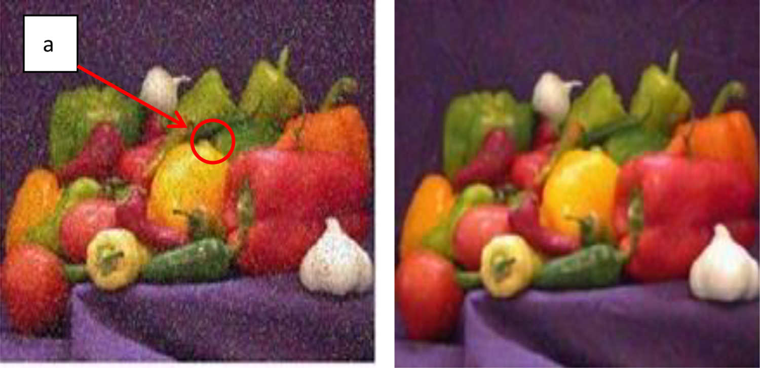
Image partial histogram and histogram smoothing process (take point “a” in Figure 7).

Conclusion

In this article, by analyzing the shortcomings of existing image processing, combined with edge detection operator and color space system and deep learning based on volume and network, the image processing model is optimized and the following conclusions are drawn:

The combination of the edge detection operator and the color space system can effectively capture the edge information and process the edge information.

The network structure of the weight sharing of the CNN significantly reduces the complexity of the image smoothing model and can automatically extract the edge features and the deformation of the image (such as translation, scaling, and tilting) after continuous deep learning. It is highly invariant. After continuous optimization and improvement, CNNs still have broad prospects in the field of image smoothing.

Footnotes

Acknowledgement

The authors would like to thank the reviewers for their constructive comments and substantial help that improved the presentation of the article.

Declaration of conflicting interests

The author(s) declared no potential conflicts of interest with respect to the research, authorship, and/or publication of this article.

Funding

The author(s) disclosed receipt of the following financial support for the research, authorship, and/or publication of this article: This work was partially supported by the National Natural Science Foundation of China under grant number 51765007, and the Guangxi Provincial Natural Science Foundation of China under grant number 2016GXNSFAA380111.

ORCID iD

Dong-yuan Ge

References

Hou

Wang

. Research and improvement of content-based image retrieval framework. Int J Pattern Recognit Artif Intell 2018; 32(12): 1850043.

Nhat-Duc

Nguyen

Tran

. Automatic recognition of asphalt pavement cracks using metaheuristic optimized edge detection algorithms and convolution neural network. Automat Constr 2018; 94: 203–213.

Yahya

Tan

, et al. Image edge detection method based on anisotropic diffusion and total variation models. J Eng 2019; 2019(2): 455–460.

Shahdoosti

Rahemi

. Edge-preserving image denoising using a deep convolutional neural network. Signal Process 2019; 159: 20–32.

Choi

Kim

Chae

, et al. Multidimensional noise reduction in C-arm cone-beam CT via 2D-based Landweber iteration and 3D-based deep neural networks. In: Medical imaging 2019: physics of medical imaging, Vol. 10948. San Diego, USA, 17–20 February 2019, pp. 1094837. SPIE.

Cai

Wen

, et al. Research on image processing of intelligent building environment based on pattern recognition technology. J Vis Commun Image Represent 2019; 61: 141–148.

De Silva

DDN

Fernando

Piyatilake

ITS

, et al. Wavelet based edge feature enhancement for convolutional neural networks. In: Eleventh international conference on machine vision (ICMV 2018), Munich, Germany, 1–3 November 2018, pp. 110412R. SPIE.

Dhar

Guha

Biswas

, et al. A system design for license plate recognition by using edge detection and convolution neural network. In: 2018 international conference on computer, communication, chemical, material and electronic engineering (IC⁴ME²), Rajshahi, Bangladesh, 8–9 February 2018, pp. 1–4. IEEE.

Wen

Sheng

, et al. Deep color guided coarse-to-fine convolutional network cascade for depth image super-resolution. IEEE Trans Image Process 2018; 28(2): 994–1006.

10.

. Convolutional Neural Network and its Applications. Dalian University of Technology, 2014; 18–22.

11.

Chang

Deng

Zhou

, et al. Convolutional neural networks in image understanding. Acta Autom Sinica 2016; 42(9): 1300–1312.

12.

Hongtao

Qinchuan

. Application of deep convolutional neural networks in computer vision. J Data Acquis Process 2016; 31(1): 1–17.

13.

Duan

, et al. Polarization application of deep recursive convolutional neural networks. Chin J Med Phys 2017; 34(3): 240–245.

14.

Guo

Jia

Guo

. Application of convolutional neural network in license plate classifier. Comput Eng Appl 2017; 53(14): 209–213.

15.

Yao

Xiang

, et al. Design of high accuracy detector for MNIST handwritten digit recognition based on convolutional neural network. In: 12th international conference on intelligent computation technology and automation (ICICTA 2019), Xiangtan, China, 26–27 October 2019, pp. 658–662. IEEE.

16.

Gao

. Optimization of lightweight convolution neural network based on automatic driving system. Comput Syst Appl 2020; 29(3): 93–99.

17.

Yoo

. Deep convolution neural networks in computer vision: a review. IEIE Trans Smart Process Comput 2015; 4(1): 35–43.

18.

Sun

Yang

Liu

. Convolutional neural network-based coarse initial position estimation of a monocular camera in large-scale 3D light detection and ranging maps. Int J Adv Robot Syst 2020; 16(6): 1–11.

19.

Xiu

. Interaction of edge-cloud computing based on SDN and NFV for next generation IoT. IEEE Internet Things J 2019; 1–9.

20.

Zhang

Huang