Sage Journals: Discover world-class research

Abstract

At present, the application of mobile robots is more and more extensive, and the movement of mobile robots cannot be separated from effective navigation, especially path exploration. Aiming at navigation problems, this article proposes a method based on deep reinforcement learning and recurrent neural network, which combines double net and recurrent neural network modules with reinforcement learning ideas. At the same time, this article designed the corresponding parameter function to improve the performance of the model. In order to test the effectiveness of this method, based on the grid map model, this paper trains in a two-dimensional simulation environment, a three-dimensional TurtleBot simulation environment, and a physical robot environment, and obtains relevant data for peer-to-peer analysis. The experimental results show that the proposed algorithm has a good improvement in path finding efficiency and path length.

Keywords

Deep reinforcement learning robot exploration recurrent neural network DDQN

Introduction

As human beings, when we want to go to a strange place, we first try to understand the environment from the starting point to the destination, and then subconsciously plan the most effective route in the brain. This principle is the core of mobile machine navigation. Abstractly, the core consists of two parts, the perceptual environment and the planned path based on the known environment.

In the early days, the emergence of simultaneous localization and mapping¹ (SLAM) technology has significant significance for mobile robot navigation. SLAM is a process in which robots are equipped with sensors such as vision, laser, and odometer to construct a map while understanding the unknown environment.^2,3 The current research method of SLAM problem is mainly by installing multi-type transmission on the robot body. The device estimates the motion information of the robot ontology and the feature information of the unknown environment, and uses information fusion to achieve accurate estimation of the pose of the robot and spatial modeling of the scene. Among them, visual SLAM,⁴ a system that uses images as the main source of contextual information. It can obtain massive and redundant texture information from the environment and has superior scene recognition capability. So it can be applied to driverless and visual enhancement. Realities and other application areas make visual SLAM a hot research direction in recent years.^5,6 The typical visual SLAM algorithm takes the estimation of camera pose as the main target and reconstructs the map by multi-view geometry theory. In order to improve the data processing speed, some visible SLAM algorithms first extract sparse image features, and then achieve inter-frame estimation and closed-loop detection through matching between feature points. However, the artificially designed sparse image features currently have many limitations. On the one hand, how to design sparse image features to optimally represent image information is still an unsolved important problem in the field of computer vision. On the other hand, sparse image features are responding to illumination changes and dynamics. There are still many challenges in terms of target motion, camera parameter changes, and lack of texture or texture in a single environment.²

At the same time, deep reinforcement learning (DRL)⁷ has become one of the most concerned directions in the field of artificial intelligence in recent years. It combines the perception of deep learning (DL) with the decision-making ability of reinforcement learning (RL) and directly controls the behavior of agents through high-dimensional perceptual input learning. It provides a new idea for solving robot navigation problems.

Among them, DL, as an important research hotspot in the field of machine learning, has achieved remarkable success in the fields of image analysis, speech recognition, natural language processing, and video classification. The basic idea of DL is to combine low-level features and form abstract, easily distinguishable high-level representations through multilayered network structures and nonlinear transformations to discover distributed feature representations of data.⁸ Therefore, the DL method focuses on the perception and expression of things.

RL, as another research hotspot in the field of machine learning, has been widely used in industrial manufacturing, simulation, robot control, optimization and scheduling, and game gaming. The basic idea of RL is to learn the optimal policy for accomplishing the goal by maximizing the cumulative reward value that the agent obtains from the environment.⁹ Therefore, the RL approach is more focused on learning strategies to solve problems.

With the rapid development of human society, in more and more complex real-world task tasks, it is necessary to use DL to automatically learn the abstract representation of large-scale input data and use this characterization as a self-incentive RL to optimize problem-solving policy. As a result, Google’s artificial intelligence research team DeepMind innovatively combines the sensible DL with the decision-making RL to form a new research hotspot in the field of artificial intelligence, namely deep reinforcement learning. Since then, in many challenging areas, the DeepMind team has constructed and implemented human expert-level agents. These agents build and learn their own knowledge directly from the original input signal, without any manual coding and domain knowledge.

At present, DRL technology has been widely used in games,¹⁰ robot control,¹¹ machine vision,^12,13 and other fields. In the field of navigation, some interesting and novel articles have appeared one after another. Gupta et al. proposed a neural architecture for navigation in a novel environment.¹⁴ Zhu et al. proposed an actor-critic model and an AI2-THOR framework to improve generalization performance and an environment with high-quality 3-D scenes and physics engines.¹⁵ Ardi et al. investigated how two agents controlled by independent deep Q-Networks interact in the classic video game Pong.¹⁶ Das et al. posed a cooperative “image guessing” game between two agents.¹⁷

The rest of the article is organized as follows. The second section is a synopsis of the basic knowledge related to DRL. The third section is the design of the model structure of this article. The experiment will be given in the fourth section. Finally, the fifth section is the summary of this article.

Related overview

RL and Q-learning

RL regards learning as a process of temptation. The reinforced learning system is mainly composed of two parts, namely, the agent and the external environment with which it interacts. The standard RL system model is shown in Figure 1. In RL, agents should choose the appropriate behavior to maximize the return on the environment. The selected action not only affects the immediate reinforcement value but also affects the state of the next moment of the environment and the final reward value.

Figure 1.

RL framework. RL: reinforcement learning.

A RL system has four main components besides agent and environment: policy, reward function, value function, and environment model.

The policy π specifies the set of actions that the agent should take in each possible state, such as the formula (1), A represents the state set at each moment, and S represents all sets of spatial states. a_t and s_t are the corresponding elements. In the policy set, we need to find the strategy $π^{*}$ that makes the problem optimal and it also called the optimal policy

π : a_{t} \in A (s_{t}), s_{t} \in S

The reward function is a reward signal obtained during the process of environmental interaction. It is a timely evaluation of a state. The reward function reflects the nature of the task faced by the agent. At the same time, it can also serve as the basis for the agent modification policy. The reward signal is an evaluation of how good or bad the action is. In practical applications, a discount reward form is usually adopted, which is described as a formula (2), where γ is a discount factor, and $0 ⩽ γ ⩽ 1$ . The r represents a single award

R_{t} = r_{t + 1} + γ \cdot r_{t + 2} + γ^{2} \cdot r_{t + 3} + ... = \sum_{k = 0}^{\infty} γ^{k} \cdot r_{t + k + 1}

The value function, also known as the evaluation function, is a measure of the distance between a state and a target state, and considers the state of a state from a long-term perspective. The state-behavior value function under a specific policy π is like the formula (3). The E represents the mean

Q^{π} (s, a) = E_{π} \{R_{t} |s_{t} = s, a_{t} = a\}

Under the optimal policy, the value function can be defined as the formula (4)

Q^{*} (s, a) = max_{π} Q^{π} (s, a)

Optimized by Bellman equation, available formula (5)

\begin{array}{l} Q^{*} (s, a) = \\ E \{r_{t + 1} + γ \cdot {max}_{a^{'}} Q^{*} (s_{t + 1}, a^{'} |s_{t} = s, a_{t} = a\} \end{array}

An important milestone in RL is the Q-learning algorithm, which was proposed by Watkins in 1989. The Q-learning algorithm is a RL algorithm that does not require an environment model and is a kind of time difference algorithm. The estimated update of its optimal action value depends on various hypothetical actions, rather than the actual actions selected based on the actual policy. The core idea is to treat the environment as a finite state discrete Markov process, representing the value of all possible actions in each state of the learning process as a value function $Q (s, a)$ , and establishing a function to store the value. Its recursive equation form is as in the formula (6)

\begin{array}{l} Q_{k + 1} (s_{t}, a_{t}) = Q_{k} (s_{t}, a_{t}) + a \cdot (r_{k + 1} \\ + γ \cdot max_{a} Q_{k} (s_{t + 1}, a_{t + 1}) - Q_{k} (s_{t}, a_{t})) \end{array}

Deep Q-learning and double Q-learning

DQN and Q-learning are both based on value iteration algorithms, but in normal Q-learning, Q-table can be used to store the Q value of each state-action when the state and action space are discrete and the dimension is not high. When the state and action space are high-dimensional continuous, it is very difficult to use Q-table storage because the action space and state are too large. So in the Q-table update can be converted into a function fitting problem, by fitting a function instead of Q-table to generate Q values, so that similar states get similar output actions. By using deep neural networks to extract complex features, DL and RL are combined to produce DQN.

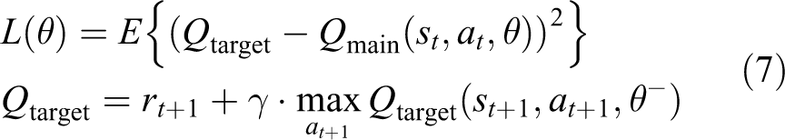
DQN does not use the Q-table to record the Q value but uses the neural network to predict the Q value and learn the optimal path of action by continuously updating the neural network. There are two neural networks in DQN: a network with a relatively fixed parameter, we call main-net, which is used to get the value of Q in main net, and another one is called target-net to get the value of Q for evaluation. The mathematical description of the loss function of DQN is as the formula (7), $θ^{-}$ is the parameter in the target network

\begin{array}{l} L (θ) = E \{(Q_{target} - Q_{main} (s_{t}, a_{t}, θ {))}^{2}\} \\ Q_{target} = r_{t + 1} + γ \cdot max_{a_{t + 1}} Q_{target} (s_{t + 1}, a_{t + 1}, θ^{-}) \end{array}

The max operation in standard Q-learning and DQN uses the same value to select and measure an action. This may actually choose too high an estimate, resulting in an overly optimistic estimate of the value. In order to avoid this situation, DDQN¹⁸ came into being. In order to reduce the impact of overestimation as much as possible, a simple method is to separate the work of selecting the optimal action from the estimation of the optimal action. The expression is as the formula (8), and the framework of this article is based on the improvement of DDQN

Q_{target} = r_{t + 1} + γ Q (s_{t + 1}, max a_{t + 1} Q (s_{t + 1}, a_{t + 1}; θ); θ^{-})

Recurrent neural network

The schematic diagram of the circulating neural network is shown in Figure 2, and C is the neural network structure, which can also be called the cyclic neural network unit. x_t and h_t are the input and output of C, respectively. The hidden layer of RNN is not only related to the current input but also related to the input features that have been experienced before. The network uses only one set of neural network structure C, and the parameters are updated by traversing time back propagation. Ordinary RNNs have gradient explosion and gradient disappearance problems, and cannot really deal with long-distance dependence. Recurrent neural network (RNN) has many derivative networks. Long short-term memory (LSTM) network is a commonly used network. LSTM replaces the fully connected (FC) hidden layer of ordinary RNN with units. Its schematic diagram is shown in Figure 3.

Figure 2.

Recurrent neural network.

Figure 3.

LSTM basic principles.

LSTM has improved the problem that ordinary RNN cannot handle long-term dependencies, adding long-term dependency C_t , input gate i_t , forgetting gate f_t formed by three Sigmoid functions σ. The output gate o_t controls the memory of past status information. In addition, gated recurrent unit (GRU) is a better variant structure of LSTM, which combines the forgotten gate and the input gate. For details, please refer to the literature.¹⁹

The combination of DL and RL in path planning

In the agent that uses the visual SLAM, the final path of the agent is still planned on the map through traditional algorithms. There are many applications for RL. Among them, the path planning part of mobile robot navigation is replaced by the RL model.

The RL model can be used to make decision-making problems after training, and realize the path selection of the agent from one location to another through the interaction between the agent and the environment. The environment is abstracted into a grid map representation. The agent can be regarded as a position state at each position of the map. The transition from one state to another corresponds to the actual movement of the entity. The choice of the agent’s state at each step corresponds to the behavioral decision-making result of the RL.

In the RL model, the reward value guides the path selection. The early Q-leaning records the reward value between the position states through the table, and then guides the next state selection through the reward value. Then, in the depth-enhanced learning, the DL model is combined, the table is replaced by the neural network, and the corresponding decision result can be obtained by inputting the state. The weighting parameters in the neural network affect the choice of the next state.

Model architecture

This article designs a novel DRL model to solve the path planning problem in navigation. We first pioneered the combination of the cyclic neural network GRU unit and the common neural network and enhanced the analysis ability of the real neural network through the memory ability of the GRU unit. Secondly, we merged the real neural network with the DRL model DDQN. The reward value function and the discount factor function for the model loss function are designed.

Environment model

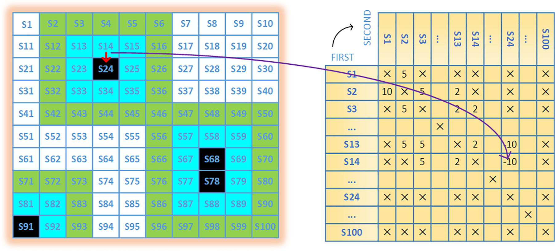
Based on the raster map model for navigation path planning analysis, this article constructs the graph model $G = < V, E >$ , where V is a finite set of nodes in the graph, and E is a finite path set between nodes in the graph, the elements are a pair. The connection of vertices is called the edge. In a complex environment, each side has a direction. G is generally a directed graph with different weights for each side. As shown in the Figure 4, where the S_i square represents each different position state, that is, the node; the data table in Figure 4 represents the transition from the state S_i to the state S_j , the reward/penalty value of the action being made, which will be fed back to the agent as a reward.

Figure 4.

Grid map construction principle. On the left is the state diagram, black is the barrier, white is the safe zone, and other colors are adjacent to the barrier. On the right is the corresponding state transition reward, such as $S_{14} \to S_{24}$ reward feedback is −10.

It is very important to strengthen the reward of the environment in the learning environment. This article designs a corresponding reward generator based on the grid map to feedback the behavior of the agent. The principle is as shown in the formula (9), where $ε < 0$ , x and y represent grid center coordinates, x_o and y_o represent obstacle center coordinates. When $s_{i} = s_{critical}$ , the reward value satisfies the 2-D normal distribution. The $s_{critical}$ is located within two compartments of the obstacle

r = \{\begin{array}{l} r_{goal}, s_{i} = s_{goal} \\ r_{obstacle}, s_{i} = s_{obstacle} \\ ε \cdot e^{- (\frac{{(x - x_{o})}^{2}}{2 σ_{x}^{2}} + \frac{{(y - y_{o})}^{2}}{2 σ_{y}^{2}})}, s_{i} = s_{critical} \\ 0, s_{i} = s_{otherwise} \end{array}

Meanwhile, depending on the environment, different discounts provided herein factors, such as the formula (10). In the formula, $γ_{obstacle} \geq γ_{goal} \geq γ_{critical} \geq γ_{otherwise}$

γ = \{\begin{array}{l} γ_{goal}, & if the area type is goal area \\ γ_{obstacle}, & if the area type is obstacle area \\ γ_{critical}, & if the area type is critical area \\ γ_{otherwise}, & if the area type is otherwise area \end{array}

Improved agent model

The overall structure of this article is based on DDQN, and on the basis of it introduces a one-to-many GRU network layer and FC layer. The GRU network has the ability to put relevant information of states to the cell units. As shown in Figure 5, the network is a double net frame that contains the main network and the target network. We enter the current state information into the main network and the next time state into the target network. Finally, the values obtained by different networks are used as the input of the loss function to obtain the error value. According to the gradient of the error, the network parameters are updated on the main network and the parameters are synchronized on the target network. When the final state decision is selected, the relevant parameters are stored in memory D. The description of this architecture is as follows:

The input data are extracted from the memory D module and the corresponding state information, that is, $s, s^{'}$ in the quaternary state $(s, a, r, s^{'})$ . $(s, a, r, s^{'})$ express shorthand $(state, action, reward, nextstate)$ .

The input is to be sent to the main network and the target network. The main network and the target network are synchronized in real time, and the network parameters are exactly the same.

The input status data are to be sent to the GRU unit. The GRU unit in the figure has eight columns. This number is for that there are eight states in the behavior set, that is, $A = [front, back, left, right, leftfront, rightfront, leftrear, rightrear]$ .

The n 8 data processed by three GRU layers, and the middle date will be sent to the FC layer of the two layers. The FC layer parameter structure is $8 64$ , $64 8$ matrix, respectively.

The activation function in the neural unit in the FC uses rectified linear unit.

In order to prevent overfitting, a dropout structure is set in the GRU layer and the FC layer, respectively.

The design of loss uses one idea in DDQN. We firstly find the action of $m a x_{a^{'}} Q (s^{'}, a^{'}; θ_{i})$ with main network ( $θ_{i}$ is the parameter of main network), then find the action in the target network. The Q value is used to form the $Q_{target}$ value. This Q value is not necessarily the largest in the target network, so we can avoid selecting the suboptimal action that is overestimated. The loss function of this article is represented by the formula (11).

The training data come from the memory pool. In this article, the training used stochastic gradient descent (SGD)²⁰ method that is a kind of local batch training way

L = E \{(r + γ \cdot Q_{target} (s^{'}, arg max_{a} (Q_{main} (s^{'}, a))) - Q_{main} (s, a {))}^{2}\}

Figure 5.

GRU-DDQN model architecture.

Experiments and results

2-D experiment

In order to verify the performance of the method, this article builds a 2-D raster map model and simulates the DDQN and GRU-DDQN examples, respectively. The experiment was carried out in grid maps of different sizes. Each group of maps was built with different obstacle coverage. The simulation program was in Python language. The computer configuration: 4-core Intel i5 7400 CPU@3.00 GHz, 8G running memory, Windows 10 operating system.

Figures 6 and 7 show the results of 10 10, 20 20 raster map simulation experiments, respectively, where the green node represents the starting point of the simulated robot and the red node represents the end point. Figures 8 and 9 correspond to Figures 6 and 7, respectively, in which the blue solid line represents the optimal path generated by the simulated robot of the GRU-DDQN example under 200 iterations in optimal path, and the yellow dotted line represents the application of the DDQN example generated under 200 iterations in optimal path. Figures 6 and 7 show the 50th and 250th paths in a comparative experiment. As can be seen from Figures 6 and 7, the GRU-DDQN example is more efficient on the global path than the DDQN study, and the path length of the search as a whole is shorter. It can be seen from Figures 8 and 9 that compared with the DDQN example, the GRU-DDQN example has a lower amplitude of oscillation and a faster convergence speed. This also demonstrates the excellent global search capabilities of GRU-DDQN. This also demonstrates the global search capabilities of GRU-DDQN. The corresponding parameter settings are as follows:

$r_{goal} = 100, r_{obstacle} = - 100, ε = - 100, σ_{x} = σ_{y} = 1$

$γ_{goal} = 0.9, r_{obstacle} = 0.9, r_{critical} = 0.8, r_{otherwise} = 0.75$

Figure 6.

10 10 Path simulation results.

Figure 7.

20 20 Path simulation results.

Figure 8.

10 10 Path convergence curve.

Figure 9.

20 20 Path convergence curve.

3-D experiment

In order to further verify the performance of the improved method, this article builds a 3-D raster map model in the second stage and simulates the DDQN and GRU-DDQN example, respectively. As shown Figures 10a and 10b, the experiment was carried out in two different simulation maps. In maps, white is a moving obstacle in each group, black is a TurtleBot simulation machine car, blue is the laser range of the machine car, and red square is the target point of a training. The computer is configured as: 4-core Intel i5 7400 CPU@3.00 GHz, 8G running memory, Ubuntu 16.04 operating system, ROS kinetic system. Part of the 3-D environment model parameters from the ROS open source community support. The corresponding parameter settings are as follows:

$r_{goal} = 500, r_{obstacle} = - 500, ε = - 50, σ_{x} = σ_{y} = 1$

$γ_{goal} = 0.9, r_{obstacle} = 0.9, r_{critical} = 0.8, r_{otherwise} = 0.75$

Figure 10(a).

3-D simulation environment.

Figure 10(b).

3-D simulation environment.

In order to analyze the performance, in the environment of Figure 10b, we conducted a comparative experiment. We recorded the specific parameters and made the corresponding maps.

As shown in Figure 11, in the Q-value map, the GRU-DDQN example has a faster convergence speed, especially in 4800 training sessions, and after 15,000 trainings, the Q value of the GRU-DDQN algorithm is still richly transformed, showing the GRU-DDQN is less likely to fall into local optimum. This demonstrates the performance of the GRU-DDQN local search. As shown in Figure 12, in the bonus map, since the GRU-DDQN example employs a multiple reward mechanism and a loop memory network, the greater reward value of the GRU-DDQN represents a lower repeated error path. As shown in Figure 13, in the loss diagram, it can be seen that the loss of the GRU-DDQN example is lower than that of the DDQN example. Figure 14 is a partial enlarged view of Figure 13. This also proves the rationality of the loss function of the model in this article. Stable parameter learning can help the model find the optimal value faster in GRU-DDQN example.

Figure 11.

Q-value comparison.

Figure 12.

Reward comparison.

Figure 13.

Loss comparison.

Figure 14.

Loss comparative enlarged view.

Physical experiment

In order to verify the performance of the model in practice, this article conducted some physical tests on the robotic machine based on the robot operating system (ROS). TurtleBot machine car is shown in Figure 15. In order to reduce the error, this group of experiments uses the TurtleBot machine car for multiple tests. The site is an obstacle zone built by the laboratory terrain. The ideal distance from the starting point to the target point is 8.3 m. After the laser environment is constructed, the environment is shown in Figures 16(a) and 16(b).

Figure 15.

TurtleBot machine car.

Figure 16(a).

Maps and paths.Maps and paths.

Figure 16(b).

Maps and paths.Maps and paths.

This article modifies the gmapping package for TurtleBot navigation and changes the manual scan to automatic scan. Based on the environment in Figure 16(a), we first performed parameter training. Except for the A* example, other examples have been trained for a certain period of time. Finally, the trained model is embedded in the navigation function package. Then we conducted five rounds of verification tests, each round was restarted. Each round consists of three experiments, and then the average is obtained based on the experimental data of this round. The result is shown in Tables 1 to 4.

Table 1.

The example of A* algorithm.

Examples	Test 1 (length/time)	Test 2 (length/time)	Test 3 (length/time)	Mean (length/time)
First round	8.9 m/74 s	9.2 m/79 s	9.2 m/75 s	9.1 m/76 s
Second round	9.4 m/96 s	9.5 m/97 s	9.9 m/98 s	9.6 m/97 s
Third round	9.5 m/90 s	9.4 m/89 s	9.3 m/85 s	9.4 m/88 s
Fourth round	8.9 m/67 s	8.8 m/62 s	9.3 m/81 s	9.0 m/70 s
Fifth round	9.3 m/83 s	9.2 m/81 s	8.8 m/76 s	9.1 m/80 s

Table 2.

The example of ANT-COLONY algorithm.

Examples	Test 1 (length/time)	Test 2 (length/time)	Test 3 (length/time)	Mean (length/time)
First round	8.7 m/71 s	9.0 m/73 s	8.7 m/72 s	8.8 m/72 s
Second round	9.3 m/85 s	9.2 m/81 s	9.1 m/80 s	9.2 m/82 s
Third round	8.6 m/70 s	8.9 m/76 s	8.6 m/79 s	8.7 m/75 s
Fourth round	9.0 m/70 s	9.1 m/80 s	8.6 m/72 s	8.9 m/74 s
Fifth round	9.2 m/79 s	9.0 m/72 s	8.8 m/71 s	9.0 m/74 s

Table 3.

The example of DDQN algorithm.

Examples	Test 1 (length/time)	Test 2 (length/time)	Test 3 (length/time)	Mean (length/time)
First round	8.8 m/77 s	9.0 m/78 s	8.6 m/73 s	8.8 m/76 s
Second round	9.3 m/86 s	9.1 m/83 s	8.9 m/74 s	9.1 m/81 s
Third round	8.9 m/68 s	8.6 m/63 s	9.2 m/70 s	8.9 m/67 s
Fourth round	9.1 m/78 s	8.9 m/73 s	8.7 m/71 s	8.9 m/74 s
Fifth round	9.2 m/80 s	9.2 m/77 s	8.6 m/77 s	9.0 m/78 s

Table 4.

The example of GRU-DDQN algorithm.

Examples	Test 1 (length/time)	Test 2 (length/time)	Test 3 (length/time)	Mean (length/time)
First round	8.8 m/65 s	8.6 m/53 s	8.7 m/56 s	8.7 m/58 s
Second round	8.8 m/63 s	8.9 m/69 s	8.7 m/60 s	8.8 m/64 s
Third round	8.7 m/66 s	8.7 m/70 s	8.5 m/68 s	8.6 m/68 s
Fourth round	8.7 m/73 s	8.8 m/65 s	8.6 m/66 s	8.7 m/68 s
Fifth round	8.4 m/71 s	8.7 m/73 s	8.4 m/69 s	8.5 m/69 s

Based on the statistics of Tables 1 to 4, it can be seen from the mean column that the GRU-DDQN study is better than other examples in terms of time consumption and path length, and searches for and selects a shorter path in a shorter time. At the same time, the stability of multiple path finding of the example is also excellent. These results reflect its efficient path finding efficiency.

Conclusions

This article introduces a novel navigation method based on DRL, which is used for path planning of agents moving in different environments. This article designs a framework that combines a recurrent neural network with DDQN. In order to improve the feasibility of the navigation method, obstacles and map rewards and discount factors are redesigned according to the environment. An improved DRL framework is then applied to the different environment to search for a reasonable route. Experiments show that the method has good performance and make path planning results more practical. Generally, the experimental results show that the proposed method reduces the global path search time by 5–8% compared to other examples in this article, meanwhile, the average path search length is shortened by 3–8%. In the future, we plan to study the effectiveness of new RL algorithms in more complex environments.

Footnotes

Declaration of conflicting interests

The author(s) declared no potential conflicts of interest with respect to the research, authorship, and/or publication of this article.

Funding

The author(s) disclosed receipt of the following financial support for the research, authorship, and/or publication of this article: This research is partly supported by the Common Key Technological Innovation Specialities of Key Industries of Chongqing Tongnan District Science and Technology Commission (Tk-2018-08), the National Natural Science Foundation of China (no. 61803058), and the Natural Science Foundation of Chongqing (cstc2018jcyjAX0385).

ORCID iD

Hao Quan

References

Khairuddin

Talib

Haron

Review on simultaneous localization and mapping (SLAM). In: IEEE international conference on control system, George Town, Malaysia, 27–29 November 2015.

Fuentes-Pacheco

Ruiz-Ascencio

Rendón-Mancha

. Visual simultaneous localization and mapping: a survey. Artif Intell Rev 2015; 43(1): 55–81.

Cadena

Carlone

Carrillo

, et al. Past, present, and future of simultaneous localization and mapping: toward the robust-perception age. IEEE Trans Robot 2016; 32(6): 1309–1332.

Strasdat

Davison

Montiel

JMM

, et al. Double window optimisation for constant time visual slam. In: 2011 international conference on computer vision, Barcelona, Spain, 6–13 November 2011, pp. 2352–2359.

Geiger

Lenz

Urtasun

. Are we ready for autonomous driving? The KITTI vision benchmark suite. In: IEEE conference on computer vision & pattern recognition, Providence, RI, USA, 16–21 June 2012.

Klein

Murray

Parallel tracking and mapping for small AR workspaces. In: IEEE & ACM international symposium on mixed & augmented reality, Nara, Japan, 13–16 November 2007.

Deep reinforcement learning. In: ICASSP 2018—2018 IEEE international conference on acoustics, speech and signal processing (ICASSP), Calgary, AB, Canada, 15–20 April 2018.

Sun

Xue

, et al. Overview of deep learning. Appl Res Comput 2012; 12: 2806–2810.

Sutton

Barto

. Reinforcement learning: an introduction. IEEE Trans Neur Netw 1998; 9(5): 1054–1054.

10.

Hosu

I-A

Rebedea

. Playing Atari games with deep reinforcement learning and human checkpoint replay. 2016. ArXiv, abs/1607.05077.

11.

Lillicrap

Hunt

Pritzel

, et al. Continuous control with deep reinforcement learning. Comput Sci 2015; 8(6): A187.

12.

Caicedo

Lazebnik

. Active object localization with deep reinforcement learning. In: Proceedings of the IEEE international conference on computer vision, Santiago, Chile, 2015, pp. 2488–2496.

13.

Meganathan

Kasi

Jagannath

Computer vision based novel steering angle calculation for autonomous vehicles. In: IEEE international conference on robotic computing, Laguna Hills, CA, USA, 31 January–2 February, 2018.

14.

Gupta

Tolani

Davidson

, et al. Cognitive mapping and planning for visual navigation. In: 2017 IEEE Conference on Computer Vision and Pattern Recognition (CVPR), Honolulu, HI, 2017, pp. 7272–7281.

15.

Zhu

Mottaghi

Kolve

, et al. Target-driven visual navigation in indoor scenes using deep reinforcement learning. In: 2017 IEEE international conference on robotics and automation (ICRA), Stockholm, 16–21 March 2016, pp. 3357–3364.

16.

Ardi

Tambet

Dorian

, et al. Multiagent cooperation and competition with deep reinforcement learning. Plos One 2017; 12(4): e0172395.

17.

Das

Kottur

Moura

JMF

, et al. Learning cooperative visual dialog agents with deep reinforcement learning. In: Proceedings of the IEEE international conference on computer vision, Venice, Italy, 2017, pp. 2951–2960.

18.

Van Hasselt

Guez

Silver

. Deep reinforcement learning with double Q-learning. Comput Sci, Arizona USA, 2016.

19.

Gers

. Learning to forget: continual prediction with LSTM. In: International conference on artificial neural networks, Edinburgh, UK, 7–10 September, 1999.

20.

Qin

Wang

, et al. Reinforcement learning for learning rate control. 2017. ArXiv, abs/1705.11159.