
Abstract
To solve the problem of understeer and oversteer for autonomous vehicle under high-speed emergency obstacle avoidance conditions, considering the effect of steering angular frequency and vehicle speed on yaw rate for four-wheel steering vehicles in the frequency domain, a feed-forward controller for four-wheel steering autonomous vehicles that tracks the desired yaw rate is proposed. Furthermore, the steering sensitivity coefficient of the vehicle is compensated linearly with the change in the steering angular frequency and vehicle speed. In addition, to minimize the tracking errors caused by vehicle nonlinearity and external disturbances, an active disturbance rejection control feedback controller that tracks the desired lateral displacement and desired yaw angle is designed. Finally, CarSim® obstacle avoidance simulation results show that an autonomous vehicle with the four-wheel steering path tracking controller consisting of feed-forward control and feedback control could not only improve the tire lateral forces but also reduce tail flicking (oversteer) and pushing ahead (understeer) under high-speed emergency obstacle avoidance conditions.
Keywords
Introduction
When the distance between an autonomous vehicle and an obstacle is less than the minimum safe distance, steering obstacle avoidance will be implemented as the longitudinal brake is not sufficient to guarantee effective obstacle avoidance. 1 Steering obstacle avoidance is similar to the “elk test.” High-speed emergency obstacle avoidance for autonomous vehicles involves two main aspects: how to achieve effective obstacle avoidance and how to improve handling stability and prevent secondary accidents. 2,3
As early as 1989, Nelson 4 proposed a quintic polynomial to describe an ideal obstacle avoidance trajectory that provided continuous curvature. Subsequently, many researchers used the trajectory to study emergency obstacle avoidance. Lee 5 studied the improvement of stability and rollover resistance in high-g lateral maneuvers. Soudbakhsh and Eskandarian 6 proposed an automated trajectory following system based on a linear quadratic method. Hassanzadeh et al. 7 used a polynomial trajectory to calculate feed-forward control inputs and used a feedback controller based on a proportional derivative (PD) controller to compensate the yaw angle error caused by nonlinearity and uncertainty in autonomous collision avoidance control. Soudbakhsh et al. 8 proposed a neighboring optimal controller for a collision avoidance system, and the entire obstacle avoidance time was controlled to be within 1.6 s. Shim et al. 9 proposed a collision-free reference trajectory and a model predictive control controller that tracks the reference trajectory. Wang et al. 10 presented a collision avoidance system consisting of a path planner and a robust tracking controller.
An active disturbance rejection control (ADRC) is used to minimize the tracking errors caused by vehicle nonlinearity and external disturbances. The ADRC can observe and compensate the external disturbances and model uncertainties without high mathematical model accuracy. The ADRC was first proposed by Professor Han Jingqing of the Chinese Academy of Sciences and further developed and improved by Professor Gao Zhiqiang of Cleveland State University. Sang et al. 11 proposed an active front steering control method that includes a PD feed-forward controller and an ADRC feedback controller. Wu et al. 12 used an active steering controller based on ADRC to follow the ideal yaw rate under high-speed emergency conditions.
The traditional four-wheel steering (4WS) vehicles use a proportional control strategy based on zero sideslip angle to become light and sensitive at low speed and stable and heavy at high speed. 13,14 Nevertheless, owing to the neglect of tracking yaw rate, these vehicles experience understeer at high speed and oversteer at low speed. 15,16 To solve the problem of understeer and oversteer for 4WS vehicles, Citroën Company (Paris, France) proposed the rear-wheel follow-up technology. Through the tilt steering principle of the drag arm suspension and the self-deflecting rubber bushing, the vehicles with peugeot steering system (PSS) technology could have an oversteer tendency at the beginning of cornering or emergency obstacle avoidance and an understeer tendency at the end of cornering or emergency obstacle avoidance. The representative vehicle type of the technology was DC7160AXC16V, but this technology was a passive control. 17 Fukui et al. 18 proposed a rear-to-front steer angle ratio based on the steering wheel operative speed: When the operative speed of the steering wheel was low, the rear wheels of 4WS vehicles were steered in the same direction as the front ones; in contrast, when the operative speed of the steering wheel was high, the rear wheels of 4WS vehicles were steered in the opposite direction to the front ones. In this article, the operative speed of the steering wheel is reflected by the steering angular frequency (ω).
The rest of this article is organized as follows. The second section describes the establishment of a 4WS vehicle model based on two-degree-of-freedom (2-DOF). In the third section, polynomial obstacle avoidance trajectories based on a ground inertial coordinate system are planned, and the trajectories are transformed into the initial inputs of an autonomous vehicle based on a vehicle coordinate system. In the fourth section, the obstacle avoidance trajectories are transformed into the initial inputs of an autonomous vehicle. In the fifth section, considering the effect of the steering angular frequency and vehicle speed (uc ) on the yaw rate, a feed-forward controller based on linear compensation is used to track the desired yaw rate, thus preventing the yaw rate reduction and the steering lag caused by the increase in ω and uc . In the sixth section, an ADRC feedback controller that tracks the desired lateral displacement and desired yaw angle is used to minimize the tracking errors caused by vehicle nonlinearity and external disturbances. The obstacle avoidance simulations are implemented in the seventh section. Finally, conclusions of this study are presented.
Linear 4WS vehicle model
To facilitate implementation and simplicity, a linear 4WS vehicle model based on 2-DOF is used to design a trajectory tracking controller. 19,20 Regardless of rolling, the state-space equation of the vehicle mode can be written as follows

where

where m is the vehicle mass, uc
is the longitudinal speed based on the vehicle coordinate system, a and b are the longitudinal distances from the vehicle center of gravity to the front and rear axles, respectively, Iz
is the yaw moment of inertia, β is the sideslip angle, r is the yaw rate, and
A vehicle model (D-class sedan) in CarSim® was used in the following obstacle avoidance simulations. The main parameters of the vehicle model are presented in Table 1.
Parameters of a D-class sedan.

CG: center of gravity
Planning of obstacle avoidance trajectories
Two coordinate systems of autonomous vehicles are shown in Figure 1(a), where OXY is a ground inertial coordinate system and oxy is a vehicle coordinate system, Ω represents the yaw angle based on the ground inertial coordinate system, the initial coordinate of obstacle avoidance is (0,0), the final coordinate of obstacle avoidance is

Obstacle avoidance diagrams: (a) two coordinate systems of autonomous vehicles and (b) a one-way four-lane road condition for obstacle avoidance.
Polynomial trajectory
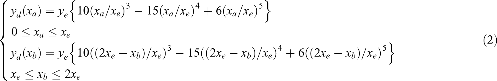
A quintic polynomial can be used to describe a desired obstacle avoidance trajectory, which is not only simple and flexible but also accurate. 22 The functions of yd on xa and xb for the desired obstacle avoidance trajectory can be expressed as follows
Cosine trajectory
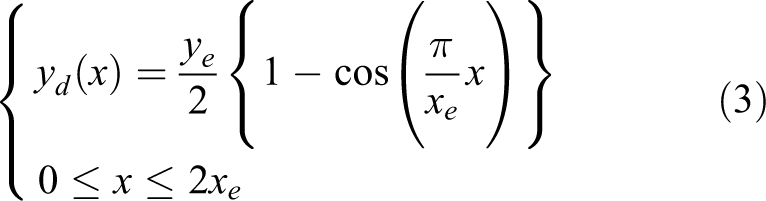
A cosine function can also be used to describe a desired obstacle avoidance trajectory. 23 The function of yd on x for the desired obstacle avoidance trajectory can be expressed as follows
Conversion effects of two different trajectories
According to the road condition in Figure 1(a), when

Conversion effects of two different obstacle avoidance trajectories: (a) lateral displacementm (b) yaw angle, (c) yaw rate, and (d) curvature.
We hope that the planned obstacle avoidance trajectory is as smooth as possible and the curvatures at the beginning and end are as close to as possible. Figure 2(d) shows that the curvatures of the polynomial trajectory at the beginning and end of obstacle avoidance are zero. Hence, in this study, the polynomial trajectory is used in the following obstacle avoidance simulations.
Initial inputs of autonomous vehicle
Considering the derivative of the function
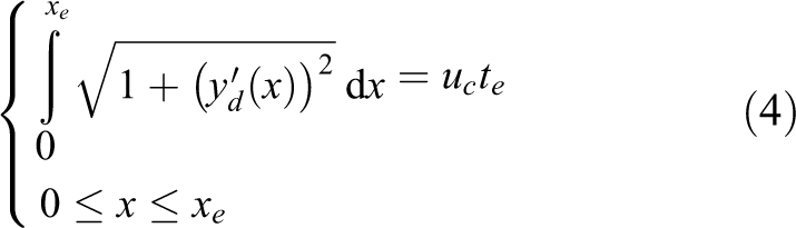
where te is the critical collision time for the obstacle avoidance trajectory.
Transforming the function

Considering the derivative of the function of
Combined with the desired yaw rate and road adhesion coefficient conditions, the desired steering wheel angle

where μ is the road adhesion coefficient,

Conversion results under four different obstacle avoidance trajectories: (a) lateral displacement, (b) yaw angle, (c) yaw rate, and (d) steering wheel angle.
As shown in Figure 3(d), the desired steering wheel angle produced by the desired obstacle avoidance trajectory is similar to a sinusoidal waveform. We can use the steering angular frequency (ω) to reflect the operative speed of the steering wheel. By comparing the black and blue lines, we can observe that ye only affects the amplitude of the desired steering wheel angle. By comparing the black, green, and blue lines, we can observe that xe and uc affect the ω and amplitude of the desired steering wheel angle.
For a front-wheel steering (FWS) autonomous vehicle, its initial inputs are formulated as follows

where
For a 4WS autonomous vehicle, the yaw rate response is generally set to a first-order lag response, and the sideslip angle response is generally set to 0. 27 Its transfer functions from the steering wheel angle to the front- and rear-wheel steering angles are expressed as follows

where s is the Laplace operator,
Feed-forward control for 4WS
The yaw rate response of the 4WS autonomous vehicle mentioned in the previous section is a first-order lag system. Its yaw rate frequency-domain response diagrams under different ω and uc conditions are shown in Figure 4, where the input is the steering wheel angle and the output is the yaw rate.

Actual yaw rate frequency-domain response diagrams under different uc
conditions: (a) sys1 represents
Figure 4 shows that the amplitude of the actual yaw rate decreases with the increase in ω, and its response lag at high speed becomes more serious. It can be observed that ω and uc have a considerable influence on the yaw rate. In the process of following the desired yaw rate rd in equation (7), the actual yaw rate for the 4WS autonomous vehicle will be lower than the desired yaw rate owing to the yaw rate frequency-domain characteristics of the 4WS vehicle in the case of large ω and high uc , thus increasing the understeer for the 4WS vehicle. For details, refer the work of Liu et al. 28
We propose a linear compensation method for the first-order yaw rate lag system to prevent the yaw rate reduction and steering lag caused by the increase in ω and uc
. This method is applied to the trajectory tracking of the autonomous vehicle as a feed-forward control. The accurate curve and error curve for the first-order yaw rate lag system under different ω conditions are shown in Figure 5, where the vertical axis (dB) represents the decibels of yaw rate response; the horizontal axis represents ω; the constraint range of ω is

First-order yaw rate frequency-domain response: (a) accurate curve and (b) error curve
To make the autonomous vehicle follow rd
accurately in the case of large ω and high uc
, combined with the
First, if the steering angular frequency is

Second, if the range of the steering angular frequency

and the decibels of the yaw rate in this state are expressed as follows

If the range of the steering angular frequency

where
Third, when

Finally, substituting the Gr value into equation (9), the front- and rear-wheel feed-forward inputs of the 4WS autonomous vehicle are expressed as follows
where
Feedback control for 4WS
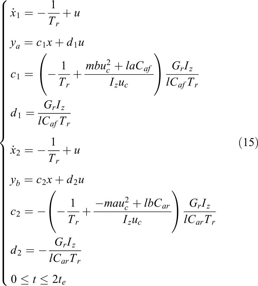
In the actual trajectory tracking process of an autonomous vehicle, uncertainties such as tire nonlinearity, load transfer, road adhesion, and crosswind disturbance seriously affect the trajectory tracking performance of the autonomous vehicle. To solve this problem, an ADRC feedback controller is used to track the desired yaw angle and desired lateral displacement and minimize the tracking errors between the actual output values and the desired values. The ADRC controller has good control effect in dealing with nonlinearity, decoupling, and time-varying problems. The ADRC controller consists of a tracking differentiator, an extended state observer (ESO), and a state error compensation law. 29 The state equation of the second-order linear control system for ADRC is expressed as

where y
1 and y
2 are the outputs of the control system, that is


where h and h
1 are the integral steps, and


The general process of the ADRC is described as follows. First, the desired target is scheduled to transition using the tracking differentiator. The purpose is to increase the adjustable ranges of the output parameters and provide effective error signals. The tracking targets values
Second, the state parameters and disturbances of the system are estimated using the ESO. The estimated target values
Third, the state errors of the lateral displacement and yaw angle are compensated dynamically by the state error compensation laws in equations (17) and (18) in real time.
Finally, the flowchart of the control algorithm of the ADRC control system is shown in Figure 6. When

Flowchart of the control algorithm of the ADRC control system.
ADRC control effects: (a) lateral displacement, (b) yaw angle, (c) lateral velocity, (d) yaw rate, (e) disturbance values, and (f) compensated values.
Obstacle avoidance simulations with CarSim
CarSim enables simulated vehicles to perform complex behaviors such as drifting and slipping under extreme conditions. Figure 8 shows animation skid marks based on large lateral slip angles generated as the vehicle slides sideways in an extreme maneuver, where the sizes of the yellow arrows indicate the magnitudes of tire forces in the lateral and vertical directions.

Tire force arrows and skid marks in an extreme maneuver.
Three different path tracking controllers
CarSim has its own path tracking controller based on an optimal preview control, named controller 1. It is located in “Steering by the Closed-loop Driver Model” of CarSim, as shown in Figure 9, where the driver preview time is 0.5 s, the driver time lag is 0 s, the low-speed dynamic limit is10 km h−1, the maximum steering wheel angle is 720°, the maximum steering wheel angle rate is 1200° s−1, and the lateral offset of the target path is Yd . The detailed control process is described in the literatures. 31,32

Optimal preview control model in CarSim®.
We expect that the controller proposed in this article is more effective than controller 1 in tracking the obstacle avoidance trajectory. Three different trajectory tracking controllers for autonomous vehicles in the following simulations are described as follows:
The only optimal preview feedback controller for an FWS autonomous vehicle is defined as controller 1, which is an FWS path tracking controller.
The only ADRC feedback control for a 4WS autonomous vehicle is defined as controller 2, which is a 4WS path tracking controller.
The feed-forward control and ADRC feedback control for a 4WS autonomous vehicle is defined as controller 3, which is also a 4WS path tracking controller.
The red, blue, and green vehicles in the following simulations represent controller 1, controller 2, and controller 3, respectively. Overall block diagrams of controllers 2 and 3 are shown in Figure 10. Considering the tire adhesion limits of 4WS vehicles, the restrictions of the simulation road and vehicle driving in the following simulations are shown as follows

where

Overall block diagrams: (a) controller 2 and (b) controller 3.
Obstacle avoidance simulation (
,
, and
)
The road simulation conditions are set as follows. The initial coordinate of the autonomous vehicle is (0,0), the initial coordinate for obstacle avoidance is (262.5,0), the coordinate of the obstacle is (300,0), and the arc length of the obstacle avoidance trajectory is 76.35 m in equation (4):

Simulation results (
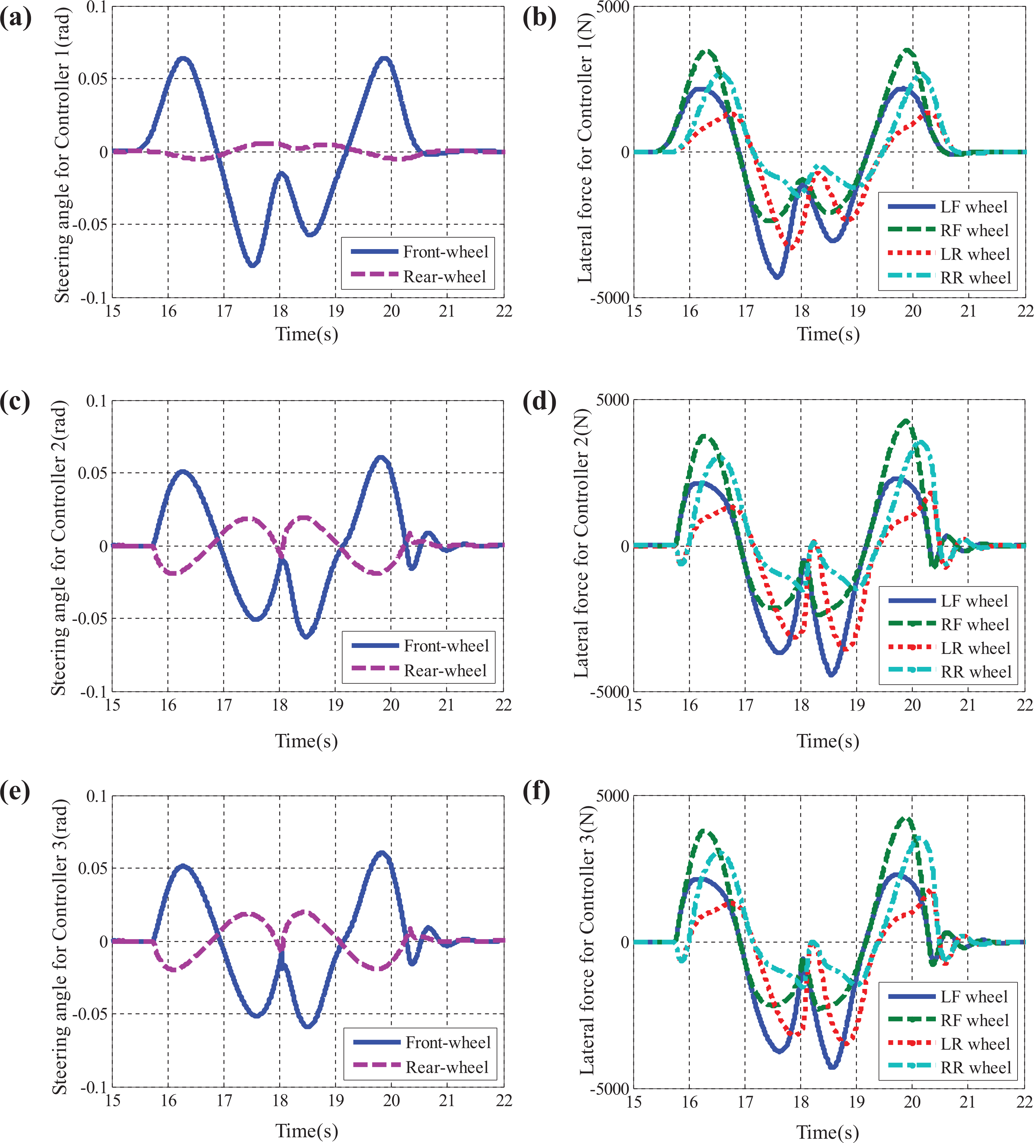
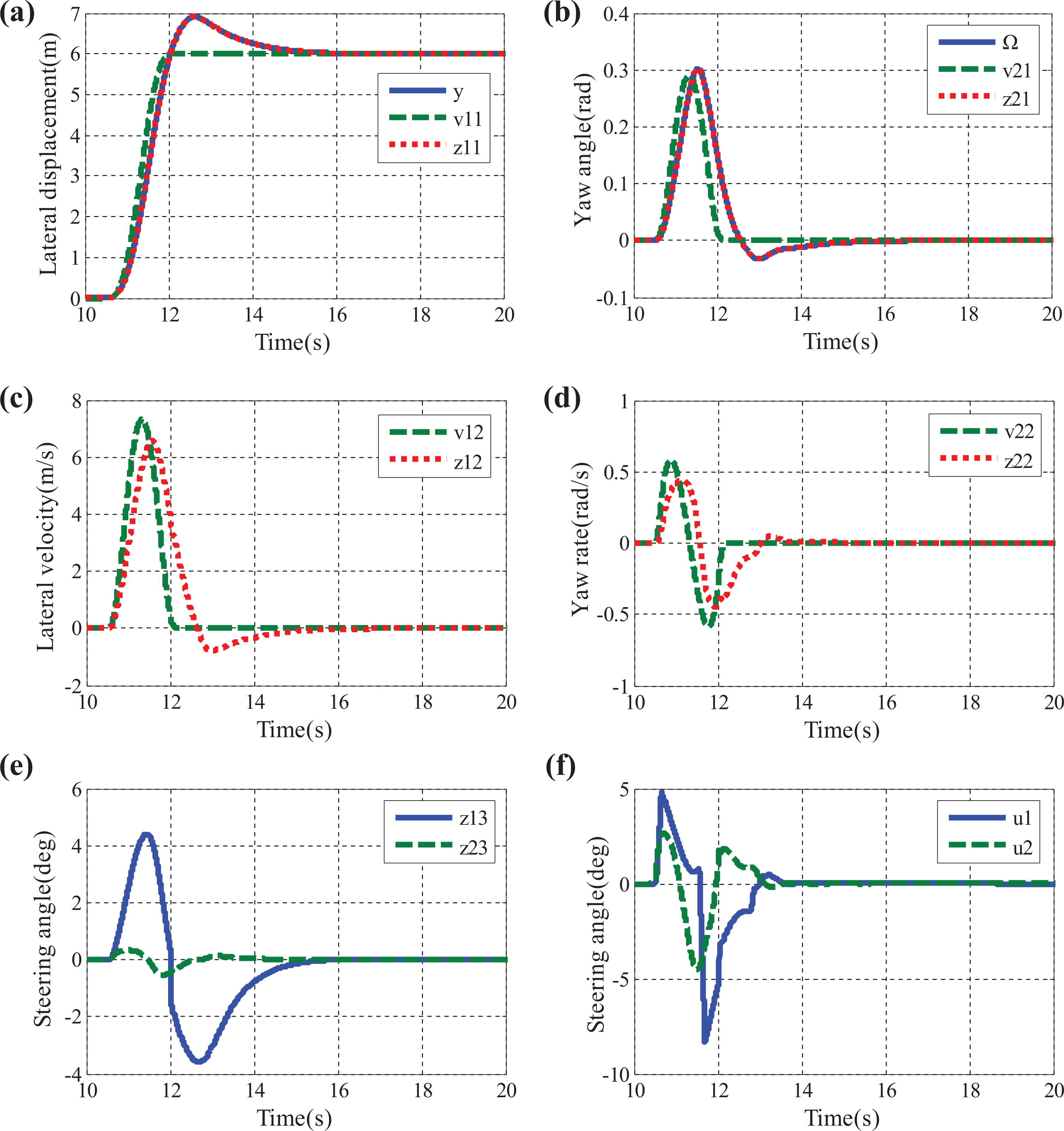
Steering angles and lateral forces (
As shown in Figures 11 and 12, the critical collision coordinates of the red, blue, and green vehicles were (18.04,6.015), (18.04,5.934), and (18.04,6.004), respectively. Even if the red and green vehicles have different front- and rear-wheel steering angles, they all achieve effective obstacle avoidance in this case, without sideslip and collision with obstacles.
Obstacle avoidance simulation (
,
, and
)
The road simulation conditions are the same as those in the “Obstacle avoidance simulation (

Simulation results (

Steering angles and lateral forces (
When uc
increased to 100 km h−1, compared to the “Obstacle avoidance simulation (
Obstacle avoidance simulation (
,
, and
)
The road simulation conditions are set as follows. The initial coordinate of the autonomous vehicle is (0,0), the initial coordinate for obstacle avoidance is (250,0), the coordinate of the obstacle is (300,0), and the arc length of the obstacle avoidance trajectory is 101.02 m in equation (4):

Simulation results (

Steering angles and lateral forces (
When xe
increased to 50 m, compared to the “Obstacle avoidance simulation (
Conclusions
The results of this study can be summarized as follows:
First, a 4WS path tracking controller can produce greater tire lateral forces than an FWS path tracking controller. Second, in terms of safety and stability under high-speed emergency obstacle avoidance conditions, the ADRC feedback controller combined with the feed-forward controller is superior to the ADRC feedback controller only. Third, for the real obstacle avoidance path tracking of 4WS autonomous vehicles, the obstacle avoidance paths can be continuously planned and updated depending on xe , uc , and ye , and the inputs of the autonomous vehicles can be adjusted by the 4WS path tracking controller in real time. Finally, in future work, the path tracking controller based on coordinated control of steering and braking for 4WS autonomous vehicles on variable-adhesion-coefficient curved roads should be further studied.
Footnotes
Declaration of conflicting interests
The author(s) declared no potential conflicts of interest with respect to the research, authorship, and/or publication of this article.
Funding
The author(s) disclosed receipt of the following financial support for the research, authorship, and/or publication of this article: This work was supported by National Natural Science Foundation of China [Grant No. 51775268] and Funding of Jiangsu Innovation Program for Graduate Education [Grant No. KYLX16_0328].