Composite clustering normal distribution transform algorithm

Abstract

Scan registration is a fundamental step for the simultaneous localization and mapping of mobile robot. The accuracy of scan registration is critical for the quality of mapping and the accuracy of robot navigation. During all of the scan registration methods, normal distribution transform is an efficient and wild-using one. But normal distribution transform will lead to the unreasonable interruption when splitting the grid and can’t express the points’ local geometric feature by prefixed grid. In this article, we propose a novel method, composite clustering normal distribution transform, which comprises the density-based clustering and k-means clustering to aggregate the points with similar local distributing feature. It takes singular value decomposition to judge the suitable degree of one cluster for further division. Meanwhile, to avoid the radiating phenomenon of LIDAR in measuring the points’ distance, we propose a method based on trigonometric to measure the internal distance. The clustering method in composite clustering normal distribution transform could ensure the expression of LIDAR’s local distribution and matching accuracy. The experimental result demonstrates that our method is more accurate and more stable than the normal distribution transform and iterative closest point methods.

Introduction

In unknown environment, simultaneous localization and mapping technology (SLAM) ¹ is the cornerstone for the autonomous and intelligence of mobile robot. ² Scan registration is a fundamental step for SLAM and autonomous navigating. ³ Surrounding information of robot is obtained by distance sensors, such as LIDAR or depth camera. Scan registration algorithm first establishes the association of two near LIDAR frames, then constructing the objective function. Finally, it will be optimized to get the transform between two LIDAR frames. With continuing scan registration, the environment model around the robot is built.

At present, there are two mostly widespread scan registration algorithms. The first one is based on iterating the closest points. The objective function is constructed by the geometric constraints of points, lines, and surfaces between two frames. The typical algorithm is iterative closest point (ICP). ⁴ The second one is based on the probability density function to build the relation. The objective function is built by the probability distributing model of current frame in reference frame. Its typical algorithm is normal distribution transform (NDT). ⁵ The main idea of this article is based on NDT method.

In this article, by analyzing the characteristic of NDT, we find that when fitting the local region of LIDAR data, NDT method will lead to unreasonable interruption while splitting points by normal distribution. Also NDT can’t express the local geometric features by prefixed grid cells. A new scan registration algorithm based on composite clustering is proposed in this article, in which the points with similar local feature in the reference frame are aggregated. The points are clustered by density-based spatial clustering of applications with noise (DBSCAN) and k-means method. DBSCAN is used to aggregate the region with continuous point distribution in reference frame. Then, the unsuitable clusters are selected by singular value decomposition (SVD)-based method and subdivided again by k-means if this cluster is unsuitable for normal fitting. The bounding box of each cluster is built for search and index. Finally, objective function of all matches is formed by normal distributing function and then optimized by trust region method.

The main contributions of this article are as follows:

We propose a novel clustering method to aggregate LIDAR points by their local features, which is a combination of density-based clustering and k-means clustering.

To judge a cluster’s suitable degree for NDT matching after DBSCAN, we propose a ratio factor based on SVD decomposition to get a cluster’s singular values.

We propose a novel distance measuring method based on trigonometric to evaluate the neighbor LIDAR points, which eliminate the LIDAR’s radiation phenomenon.

This article is organized as follows. In “Related work” section, we discuss the related work about scan registration. In “Problem statement” section, the basic procedure of NDT is narrated, and the disadvantage of original NDT method is discussed. Section “Composite clustering scan registration” is the main text of this article, and the overall procedure of composite clustering NDT (CCNDT) is narrated in detail. In “Experiments” section, the comparing experiments among CCNDT, NDT, and ICP are designed and discussed. The last section is a brief conclusion of this article.

Related work

LIDAR is a main exteroceptive sensor in mobile robot ⁶ when acquiring distance data from the robot’s surrounding. In contract with wheel odometer and IMU, LIDAR information represent the correlation between robot and environment. With the map built by LIDAR data, robot can realize where it locates and where it is the destination and path. Scan registration is a method to get the transform between LIDAR frame, which is critical for robot.

Scan registration aims to construct the relation of two LIDAR frames by matching their points, then building the objective function and optimizing. The most representable scan registration methods are ICP and NDT methods.

ICP is first proposed by Besl and Mckay, ⁴ in which the frame relation is built by matching the closest point pairs. But without additional information such as geometric characteristics, the matching is worse when there is a large transform. Then, Segal et al. ⁷ propose a general ICP method using the local inner points to get the face structure, which makes the result more accurate. Serafin and Grisetti ^{8 –10} use the surface characteristics around the points to search for ICP corresponds. Cox and colleagues ¹¹ extract line features from LIDAR data and match the points with relevant lines. Iterative dual correspondence method ¹² is used to improve matching accuracy by maintaining two relevant sets. Wang et al. ¹³ come up with a multilayer matching method to deal with the data-association problem, in which the uncertainty of the matching results is described by Fisher information matrix. MbICP ¹⁴ is designed to improve convergence with large initial orientation errors, which explicitly put a measure of rotational error as part of the distance metric. Those ICP methods are easy to deploy and use, but their two weaknesses ¹⁵ are considerable: the nearest match is not correct matching in many conditions and the computing cost is very heavy when searching the nearest points.

To avoid the heavy matching of ICP, Biber and Strasser ⁵ come up with the probability-based method named as NDT (normal distribution method). It divides the reference frame into grid cells. Then, the normal distributing parameter is calculated for each cell. Next, each point of current frame is matched with a grid by their coordinate to get the probability density. With this method, it needn’t match each point but the grid cells to reduce computational cost. Moreover, normal distribution can provide the geometric representation of points, which gives the higher order derivatives for optimizing. ¹⁶

Based on NDT, Gutmann and Konolige ¹⁷ registrant current frame with serval previous frame to improve precision. Mitra et al. ¹⁸ use quadratic approximants to get the distance from target surface, describing the model surface implicitly. Ulas and Temeltas ¹⁹ come up with a feature-based NDT method. Kunjin Ryu et al. ²⁰ use ND-to-ND method to get global matching, which can not only provide the internal frames transform but also be used for loop closure detection ²¹ for graph optimization. Gouveia et al. ²² use the multithreading to parallelize the data fusion step. Even more, Bosse et al. ¹⁶ match all the LIDAR frames by registering the subregions and global map. And in kinect fusion by Newcombe et al., ²³ the relationship is built by a global optimizing model, but it is too heavy and slow for most calculating platforms. There are also many other scan-matching methods such as expectation-maximization (EM) matching method by Thrun et al. ²⁴ and the graph model method by Feng and Milios. ¹²

Problem statement

Compared with other scan registration methods, NDT has the following two advantages when building the correlation:

1. The normal distributing model gives the points in one cluster a common attribute, which reduces the quantity in matching.

2. Compared with the error function of point distance, the normal distributing error function has higher-order derivation, which makes it possible to use the optimizing method with the second-order gradient.

The scheme of NDT includes three parts, as shown in Figure 1. Firstly, the points in reference frame are divided into grid cell and constructed the normal distribution of the points in each cell. Then, the points of current frame are linked with those cells by their relevant coordinate. Finally, the error of those links is minimized to get the transform. Next, we’ll have an elaborate narration of the inference.

Figure 1.

Schematic illustration of NDT method. When a robot moves from x ¹ to $x^m$ , its LIDAR sensor will capture the LIDAR points Pⁱ of surrounding in each pose. And NDT method will build the relationship between points and grid cells of two neighbor LIDAR frames, such as $P^{m-1}$ and $P^m$ . Then, the transform relation will be calculated by objective function. NDT: normal distribution transform.

When the robot moving, distance points are obtained from LIDAR. Let $P^m=\left\{p_i^m |\forall i\in \left\{1,\dots n_m\right\}\right\}$ and $P^{m-1}=\left\{p_i^{m-1}=\left[\begin{array}{cc}x& y\end{array}\right] |\forall i\in \left\{1,\dots n_{m-1}\right\}\right\}$ individually represent the current and previous frames indexed by $m,m-1$ , and the point number is denoted by i. Scan registration aims to get the coordinate transform ${\Delta }^{m\to m-1}={\left[\begin{array}{ccc}{x}_{\Delta }& y_{\Delta }& {\theta }_{\Delta }\end{array}\right]}^T$ , where $x_{\Delta },y_{\Delta }$ is a plane transform and ${\theta }_{\Delta }$ is rotation. In this article, we use “reference frame” to represent the previous frame $P^{m-1}$ .

In NDT method, the reference frame is first divided into grids, as shown in Figure 2. In advance, it needs to get the grid span in vertical and horizontal. Then, the frame is divided into span distance and cell interval. The values of span distance and cell interval are manually tuned.

Figure 2.

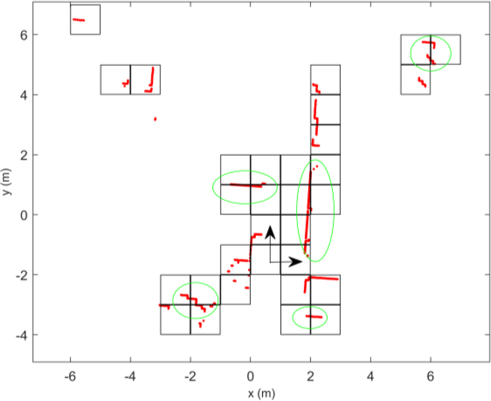
Grid splitting illustration with LIDAR data from ACES building at the University of Texas. The points as green ellipse marked should belong to one collection, but they are divided into different grid cells by NDT. Where the red points are LIDAR points, the arrows indicate the robot’s position. NDT: normal distribution transform.

Each point will be filled into cells according to their inclusion relation. Then, each cell is represented by normal parameter. For instance, the parameter of points in one cell is

${}^{(i,j)}\overline{z}{}^{m-1}=\frac{1}{n}{\displaystyle \sum }_{k=1}^n{}_{ }{}^{(i,j)}p{ }_k^{m-1}$

1

${}_{ }{}^{(i,j)}\epsilon { }_k^m=\mathcal{T}\left({}_{ }{}^{(i,j)}p{ }_k^m,{\Delta }^m\right)-{}_{ }{}^{(i,j)}\overline{z}{}^{m-1}$

2

${}_{ }{}^{(i,j)}\overline{\Sigma }{}^m=\frac{1}{n}{\displaystyle \sum _{k=1}^n}{}_{ }{}^{(i,j)}\epsilon { }_k^m{\left({}_{ }{}^{(i,j)}\epsilon { }_k^m\right)}^T$

3

where ${}^{(i,j)}\overline{z}{}^{m-1}$ is the mean of the points in grid cell $\left(i,j\right)$ , and the sign $\left(i,j\right)$ on the top left is the grid cell’s index, which means the cell located at ith row and jth column. The sign m or $m-1$ on top right is time index of LIDAR data. $p_k$ is the coordination of point k. ${\Delta }^m$ is transform parameter to be optimized from pose $m-1$ to m. And $\overline{\Sigma }$ is covariance of the cell. And $\mathcal{T}\left(p,\Delta \right)$ is a transform operator as explicitly shown as

$\mathcal{T}\left(p,\Delta \right)=\left[\begin{array}{cc}\text{cos }{\theta }_{\Delta }& -\text{sin }{\theta }_{\Delta }\\ \text{sin }{\theta }_{\Delta }& \text{cos }{\theta }_{\Delta }\end{array}\right]\left[\begin{array}{c}{x}_p\\ y_p\end{array}\right]+\left[\begin{array}{c}{x}_{\Delta }\\ y_{\Delta }\end{array}\right]$

4

Here the coordinate of p is $\left[x_p,y_p,{\theta }_p\right]$ , and the coordinate of Δ is $\left[x_{\Delta },y_{\Delta },{\theta }_{\Delta }\right]$ .

With the reference frame has been represented by normal distribution, the point in current frame can be linked to the reference cells. The current frame is transformed to the coordinate of reference frame with the initial value from Odometer or IMU. If no input source, initial value will be set as ${\Delta }_{init}^{\text{m}}={\left[\begin{array}{ccc}0& 0& 0\end{array}\right]}^T$ . Then, each point $p_k^m$ in current frame is linked to a relevant grid cell by coordinate. The point’s error function is obtained by normal distributing density function

$\begin{array}{l}{}^{\left(i,j\right)}{f}_k^m={\eta }_{\text{norm}}\\ \hspace{0.17em}\hspace{0.17em}\hspace{0.17em}\hspace{0.17em}\hspace{0.17em}\hspace{0.17em}\hspace{0.17em}\hspace{0.17em}\hspace{0.17em}\hspace{0.17em}\hspace{0.17em}*\text{exp}\left({\left({}^{\left(i,j\right)}{\epsilon }_k^{m-1}\right)}^T{\overline{\Sigma }}_{i,j}^{m-1}\left({}^{\left(i,j\right)}{\epsilon }_k^{m-1}\right)\right)\end{array}$

5

${\eta }_{\text{norm}}={\left({\left(2\pi \right)}^2\text{det}\left({}_{ }{}^{(i,j)}\overline{\Sigma }{}^{m-1}\right)\right)}^{-\frac{1}{2}}$

6

where f is a normal distributing probability density from points k to grid cell $\left(i,j\right)$ .

And the overall objective function is

$\text{log}{f}^m={\displaystyle \sum _{k\in P^m}}\text{log}{}^{(i,j)}{f}_k^m$

7

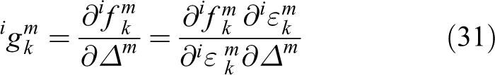
The gradient and Hessian of objective function are calculated to optimize the displacement of the two robot poses, which will be deduced in “Range-based decomposition” section. Then, Newton method is used to optimize the transform parameter

${\Delta }^m=-{\left(H^m\right)}^{-1}{g}^m$

8

Here, g^m is the gradient of overall objective function, and H^m is its Hessian matrix.

The inference above is NDT’s scan-matching procedure. It is ingenious to use normal distribution to represent the reference LIDAR frame. Thus, the optimizing step could utilize the normal probability density function to get the first-order and second-order derivatives.

But while using NDT method in real LIDAR data, it is found that the points should belong to one cluster according to their local feature, but they are split unsuitable by prefixed grid boundary, which make points aggregate to the wrong cluster.

As shown in Figure 2, the LIDAR frame should be divided into 20 local sets according to its local shape but resulted into 31 by the fixed interval division of NDT, where the unsuitable split is 35.5%.

As shown in Figure 3, the left figure illustrates the points are divided based on their local distributing feature, the set’s center is same as the points’ centroid. Then, as shown in the arrow of Figure 3(a), the new point will get good match with the cluster. But the ineligible division in Figure 3(b) will lead to unreasonable matching, where points are divided by the prefixed boundary, like NDT method, and the point after matching can’t link with the target cluster’s centroid. So, the precision of NDT is limited by the prefixed grid boundary, which can’t adapt to the local distribution’s variety.

Figure 3.

Example of suitable (left) and unsuitable (right) splitting results. The orange dots are the LIDAR points in current frame, and the green and blue dots are the points in reference frame. Each arrow represents a matching result. And the boundary of grid cell is denoted as blue line. (a) Left: the points are divided based on their local distributing shape. (b) Right: the points are divided by prefixed boundaries, like NDT method, which can’t link to the centroid of cluster after matching. NDT: normal distribution transform.

The core thought of our method is motivated by the disadvantage of ineligible grid splitting of NDT. To deal with this problem, we compose a new point dividing method based on composite clustering, which can adapt to the local distribution of LIDAR points. In this way, the accuracy of scan registration is improved as shown in the “Experiment” section.

Composite clustering scan registration

Algorithm overview

The scheme of CCNDT method is introduced summarily, of which the core goal is to get the transform between two robot poses by their LIDAR and Odometer data. As shown in Figure 4, the whole process includes five steps:

Figure 4.

The scheme of CCNDT method. Where the inputs are current frame and reference frame, the output is the transform between two LIDAR frames. The reference frame is processed by DBSCAN clustering, SVD selection, and k-means clustering. Then, the normal distributing parameters are calculated and matched with the current frame by bounding box. Finally, with the matching indexes, the transform between two LIDAR frames can be calculated. CCNDT: composite clustering normal distribution transform; DBSCAN: density-based spatial clustering of applications with noise; SVD: singular value decomposition.

1. It is started from the reference frame, where the inputted reference LIDAR data are first processed by the density clustering (see “Local distributing-based clustering” section). And the trigonometric-based distance method (see “Distance measuring method-based on trigonometric function” section) is used to measure the interval between each point. The reference LIDAR points are clustered by their local distributing shape.

2. The outputted clusters from (1) are filtered by SVD method to judge their eligible degree. Otherwise, the ineligible clusters will be further divided (see “Range-based decomposition” section).

3. After the filter process, the ineligible cluster will be divided into k‘s small cluster by k-means method. The value of k is proportional to the ratio scale of this cluster’s singular values (see “Range-based decomposition” section).

4. Each clustering result will be given a bounding box for matching. Those points in current frame can be mapped into the bounding box by their relative coordination (see “Registration and objective function” section).

5. With the links from current frame’s points to reference frames’ clusters, the objective function is obtained by gathering each link’s normal distribution error. The transform between these two LIDAR frames is calculated by the objective function (see “Optimization and solving” section).

In the next several sections, we will walk through each of those steps in detail.

Local distributing-based clustering

The characteristic of LIDAR points should be analyzed firstly. LIDAR is a surveying sensor, as shown in Figure 5, which measures distance to a target by pulsing laser light and measuring the flying time from launching to receiving the reflected pulses by a laser receiver. LIDAR will record each measurement’s angle and distance when rotating. So, the obstacle in the laser illuminating path will be captured.

Figure 5.

LIDAR measure object’s position by flying time. Where the red line denotes the LIDAR’s beam. The LIDAR is located at the center of the radius in dark circle. The blue shapes are obstacles in the surrounding.

As shown in Figure 5, LIDAR points captured from the wall-like shape will form a straightline LIDAR distribution and from the cylinder shape will form an arc distribution. To make those points from same region clustered together and from different regions separated, it needs to get a method to identify the similarity and otherness among each object.

As the continuous of object boundary, the LIDAR point from the same obstacle is more continuous and has a higher reachable density than other areas. This condition is suitable for the density-based clustering named DBSCAN, ²⁵ in which the points from the same cluster have a higher density than from the different clusters. DBSACN provides a model named “Density Reachability,” which selects points satisfied the distance thresholds into one cluster. It is good at clustering the points in arbitrary distributing shapes.

In DBSCAN, $D_1^{m-1}$ is an initial cluster, and put into a father point $p_x^{m-1}$ , which is randomly fetched from the reference frame $P^{m-1}$ . Then it is going to find out all the points in $P^{m-1}$ satisfied with the limitation:

$\Vert p_i^{m-1}-p_x^{m-1}<\beta \Vert$

9

where β is the distance threshold. In “Distance measuring method based on trigonometric function” section, we will introduce a new method to initialize and calculate this threshold.

And the points satisfied with the limitation are put into set $D_1^{m-1},$ meanwhile, removed from $P^{m-1}$ . After ending a traversal round, the next turn starts with all the points from the last turn as the father points of this turn. Then, it continues searching until no more new point added in during a new turn, as shown in Figure 6. So far, a density cluster $D_1^{m-1}$ is formed.

Figure 6.

Searching for the points belonging to one set with DBSCAN. The dash lines are the searching boundary. The red points belong to one density cluster. DBSCAN: density-based spatial clustering of applications with noise.

For the left points in $P^{m-1}$ , the above iterating procedure will be repeated until emptying $P^{m-1}$ . Finally, a series of sets $\left\{{\mathfrak{D}}^{m-1}\right\}$ are constructed

$\left\{{\mathfrak{D}}^{m-1}\right\}=\left\{D_1^{m-1}{D}_2^{m-1}{D}_3^{m-1}\dots D_n^{m-1}\right\}$

10

Each of those clusters has two characteristics. (1) The points in one cluster are density connected within threshold β. (2) All of the density reachable points from one cluster must belong to this cluster.

If the points in one cluster are too few $N_{D_i^{m-1}}<\zeta$ , it will be improper for normal distributing fitting, where $N_{D_i^{m-1}}$ is the number of points in cluster $D_i^{m-1}$ , and ζ is an adjusting parameter depend on the resolution of LIDAR. When the LIDAR’s angular resolution is 0.25°, we set $\zeta =3$ . So, these clusters will be deleted and their points will be collected into a special cluster named $D_0^{m-1}$ . Then the series of clusters become $\left\{{\mathfrak{D}}^{m-1}\right\}=\left\{D_0^{m-1} D_1^{m-1} D_2^{m-1} \dots D_n^{m-1}\right\}$ .

Distance measuring method based on trigonometric function

After clustering LIDAR points by DBSCAN, we find a disappointed weakness. As the radiating phenomenon of LIDAR, the LIDAR points from the straight facet would not be uniformly distributed in a line. The LIDAR point captured on the same object from different distance will be sampled in different interval, as shown in Figure 7. The nearby interval is close and the further interval is distant. So, the threshold β is unsuitable to be a constant when measuring the points interval.

Figure 7.

Radiation of the laser beam from a straight obstacle. The interval will be formed as the nearly points density and the further points sparsity.

Here, we use a new method based on trigonometric function to measure the density reachability. When starting a new cluster, there is only one initial father point in the cluster. So, it just needs to consider the distance. And the threshold β is

$\beta ={\rho }_0\text{sin}\Delta \theta$

11

where Δθ is the LIDAR’s angular resolution, and ${\rho }_0$ is the distance of father point, as shown in Figure 8.

Figure 8.

The measurement after initializing, where o is the LIDAR center and $o\text{'}$ is the pedal from LIDAR to the object’s facet. Points $p_0, p_1$ are the Father points obtained from initial step. p ₂ is the next candidate point to be measured. a is the angle of $\angle p_0{p}_{1}o$ .

After the initial procedure, the value of angle a can be obtained by the law of cosines with the initial points

$\text{cos}a=\frac{l_{o{p}_0}^2+l_{p_0{p}_1}^2-l_{o{p}_1}^2}{2l_{p_0{p}_1}{l}_{o{p}_1}}=\frac{{\rho }_0^2+{\rho }_1^2-\Vert {\rho }_0{\rho }_1\Vert {}_2^2}{2\Vert {\rho }_0{\rho }_1{\Vert }_2{\rho }_1}$

12

where the formula is based on the law of cosines, and $l_{p_0{p}_1},l_{o{p}_0}={\rho }_0,l_{o{p}_1}={\rho }_1$ is the edge of triangle $\Delta o{p}_0{p}_1$ .

Then, in triangle $\Delta o{p}_1{p}_2$ with two angles and one edge known, it is easy to calculate other parameters with the trigonometric function. We can get the distance method based on the trigonometric relation

$\beta =l_{p_1{p}_2}=\frac{{\rho }_1\text{sin }a}{\text{cos }\left(\Delta \theta -a\right)}-{\rho }_1\text{cos }a$

13

where β means that if the third point is collinear with the two initial points, the distance of $p_1{p}_2$ should be $l_{p_{2}o}$ in theory, as shown in Figure 8.

Finally, the combined distance measuring threshold is

$\begin{array}{l}\beta =\{\begin{array}{cc}\lambda {\rho }_i\sin \Delta \theta & \text{if not initial}\\ \lambda \frac{{\rho }_1\text{sin }a}{\text{sin}\left(\Delta \theta -a\right)}-{\rho }_1\text{cos }a& \text{if initial}\end{array}\\ \lambda =1+\Vert Q_{\text{LIDAR}}{\Vert }_{\text{2}}\end{array}$

14

where $Q_{\text{LIDAR}}$ is the covariance of LIDAR’s accuracy, and the covariance can be obtained by calibrating the LIDAR. And λ is the adjustment factor for LIDAR’s physical noise.

As an example, to show the result after density clustering, one LIDAR scan of the ACES building is tested, which contains 1081 points. And after applying the density clustering and our trigonometric distance method, the LIDAR points are divided by their local distribution properly, as shown in Figure 9.

Figure 9.

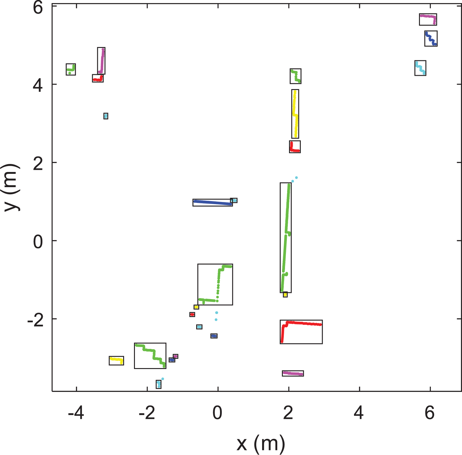
Example of LIDAR points after DBSCAN clustering with trigonometric distance method. Each box region represents a point cluster. DBSCAN: density-based spatial clustering of applications with noise.

Range-based decomposition

After DBSCAN processing, the continual regions of LIDAR data have been aggregated together, as shown in Figure 9. But on the one hand, as the larger cluster has a larger bounding box, so a point may be included by this bounding box but far from the cluster’s center, which will lead to heavy distorted links. On the other hand, the larger cluster has a strong attraction for its nearby points than a smaller cluster, which is because the weight of one cluster is in direct proportion to its quantity of points. And it will make the relaxing iteration unbalance. So, the result of DBSCAN is unsuitable for matching till now.

It needs to further decompose the larger cluster. The first question is how to select out the unsuitable clusters. It is noticed that such kind of clusters not only have a wider boundary but also have a big disparity of primary and secondary eigenvalues. So, each cluster in $\left\{{\mathfrak{D}}^{m-1}\right\}$ first be performed with SVD to get its singular values

$U{\Sigma }_{\text{singular}}{V}^T=\text{svd}\left({}_{}{}^i\overline{\Sigma }{}^{m-1}\right)$

15

where ${}_{}{}^i\overline{\Sigma }{}^{m-1}$ is the covariance of $D_i^{m-1}$ . And ${\Sigma }_{\text{singular}}$ = diag (σ₁,σ₂,σ₃) is the singular values of covariance ${}_{}{}^i\overline{\Sigma }{}^{m-1}$ .

The ratio from the biggest to the second singular value can denote the ineligible degree of one cluster.

$\xi =\frac{{\sigma }_1{}^2}{{\sigma }_2{}^2}$

16

where ${\sigma }_1$ and ${\sigma }_2$ are the primary and secondary singular values of the cluster’s covariance, respectively. ξ is the ratio factor. If the ratio factor is bigger than 2, it means the larger cluster should be divided into two smaller clusters at least. Otherwise, it doesn’t need to be divided. So, if $\xi >2$ , the cluster’s shape is disproportion and unsuitable for normal fitting. Then, it is necessary to get a further division for those unsuitable clusters.

The second question is how to further divide the unsuitable clusters. Those larger clusters can be divided by k-means method ²⁶ into k smaller clusters. k-Means makes their inner distance of one cluster minimum and their outer distance maximum. The unsupervised learning method of k-means can adaptively select the coordinate of initial points. And with the Euclidean distance, the shapes of clusters outputted from k-means are suitable for normal fitting.

And its most important parameter is the clustering quantity k. Here, we use the previous SVD result to calculate the value of k

$k_i^{m-1}=\text{round}\left(\xi \right)$

17

where $k_i^{m-1}$ is the clustering number of the ith cluster in the $m-1$ LIDAR frame. ξ is the ratio factor.

The result of k-means is

$\left\{D_{i,1}^{m-1},D_{i,2}^{m-1}\dots \dots D_{i,k}^{m-1}\right\}=k-\text{means}\left(D_i^{m-1},k_i^{m-1},\text{dis}\right)$

18

where $D_i^{m-1}$ is decomposed into k clusters $\left\{D_{i,1}^{m-1},D_{i,2}^{m-1}\dots \dots D_{i,k}^{m-1}\right\}$ with Euclidean distance method $\text{dis}=\Vert p_i-p_j\Vert$ .

The cluster with few numbers of points also needs to be removed and puts into $\left\{D_O^{m-1}\right\}$ as mentioned in “Local distributing-based clustering” section. The cluster $\left\{D_O^{m-1}\right\}$ is useful when a point can’t match with any cluster, then the points in $\left\{D_O^{m-1}\right\}$ can be an optional candidate to build the matching relation.

As an illustration, we select the unsuitable clusters in Figure 9 by SVD ratio factor, then applying k-means method to divide those unsuitable clusters. The change from Figure 9 to Figure 10 demonstrates that the unsuitable clusters are decomposed into smaller clique by k-means. Each of the clusters as the box marked in Figure 10 is more balance in each direction, which is more suitable for normal distribution fitting.

Figure 10.

Example of LIDAR clusters after k-means clustering. Each box region represents a set of clustered points. Those clusters are first selected by SVD-based method, then the unqualified clusters are further divided by k-means. SVD: singular value decomposition.

Till now, there are two groups of the cluster: the first group is the suitable results of DBSCAN and the second group is those unsuitable clusters decomposed by k-means. Then reorder them as

$\begin{array}{l}\left\{D_i^{m-1},D_{c+1}^{m-1}\dots \dots D_{c+n-1}^{m-1}\right\}\\ =\text{reorder}\left\{D_{i,1}^{m-1},D_{i,2}^{m-1}\dots \dots D_{i,n}^{m-1}\right\}\end{array}$

19

where c is the number of elements in $\left\{{\stackrel{\sim }{\mathfrak{D}}}^{m-1}\right\}$ , which means the first cluster $D_{i,1}^{m-1}$ replaces its parent index $D_i^{m-1}$ , and the rest clusters $\left[2,3\dots n\right]$ are added after the latest index c.

For uniform, those two groups of clusters are integrated together and denoted as

$\left\{{\stackrel{\sim }{\mathfrak{D}}}^{m-1}\right\}=\left\{{\stackrel{\sim }{D}}_1^{m-1} {\stackrel{\sim }{D}}_2^{m-1} {\stackrel{\sim }{D}}_3^{m-1}\dots {\stackrel{\sim }{D}}_n^{m-1}\right\}$

20

This step just changes the index of the clusters for their lower right corner.

Registration and objective function

After obtaining the proper clusters, here it is going to inference their matching parameters. As the origin NDT method inferred in “Problem statement” section, the normal distributing parameter of each cluster includes its mean and covariance. The mean of cluster $D_i^{m-1}$ is

${}_{ }{}^i\overline{z}{}^{m-1}=\frac{1}{n}{\displaystyle \sum _{k=1}^n}{}_{ }{}^{i}p{ }_k^{m-1}$

21

where ${\left.{}_{ }{}^{i}p{ }_k^{m-1}\right|}_{\left\{k=1,2\dots n\right\}}\in D_i^{m-1}$ , and i is the index of cluster.

And its covariance is

${}_{ }{}^i\overline{\Sigma }{}^m=\frac{1}{n}{\displaystyle \sum _{k=1}^n}{}^i\epsilon k^m{\left({}^i{\epsilon }_k^m\right)}^T$

22

When building the matching relation, the original NDT method uses grid cells to link the points and the clusters. But in CCNDT, the cluster’s size and position are not regular, so here we use the bounding box as shown in Figure 11, for searching.

Figure 11.

The bounding box of one cluster, where $\underset{y}{\text{min}}{\stackrel{\sim }{D}}_i^{m-1},$ $\underset{y}{\text{max}}{\stackrel{\sim }{D}}_i^{m-1},$ $\underset{x}{\text{min}}{\stackrel{\sim }{D}}_i^{m-1},\underset{x}{\text{max}}{\stackrel{\sim }{D}}_i^{m-1}$ is the coordinates of the boundary points in this cluster, and α is the marginal width initialized as in equations (23) and (24).

$\alpha =\sqrt[2]{\frac{\text{areas}\left({\stackrel{\sim }{D}}_i^{m-1}\right) }{\text{quantity}\left({\stackrel{\sim }{D}}_i^{m-1}\right)}}$

23

$\begin{array}{l}\text{area}\left({\stackrel{\sim }{D}}_i^{m-1}\right)=\left(\underset{y}{\text{max}}{\stackrel{\sim }{D}}_i^{m-1}-\underset{y}{\text{min}}{\stackrel{\sim }{D}}_i^{m-1}\right)\\ \hspace{0.17em}\hspace{0.17em}\hspace{0.17em}\hspace{0.17em}\hspace{0.17em}\hspace{0.17em}\hspace{0.17em}\hspace{0.17em}\hspace{0.17em}\hspace{0.17em}\hspace{0.17em}\hspace{0.17em}\hspace{0.17em}\hspace{0.17em}\hspace{0.17em}\hspace{0.17em}\hspace{0.17em}\text{*}\left(\underset{x}{\text{max}}{\stackrel{\sim }{D}}_i^{m-1}-\underset{x}{\text{min}}{\stackrel{\sim }{D}}_i^{m-1}\right)\end{array}$

24

where $\text{area}\left({\stackrel{\sim }{D}}_i^{m-1}\right)$ is the area of this cluster and $\text{quantity}\left({\stackrel{\sim }{D}}_i^{m-1}\right)$ is the number of points in this cluster.

For each cluster ${\stackrel{\sim }{D}}_i^{m-1}$ in $\left\{{\stackrel{\sim }{\mathfrak{D}}}^{m-1}\right\}$ , its bounding box is denoted as

${\mathbb{B}}_i=\left[\begin{array}{c}\left(\underset{x}{\text{min}}{\stackrel{\sim }{D}}_i^{m-1}-\alpha ,\underset{y}{\text{min}}{\stackrel{\sim }{D}}_i^{m-1}-\alpha \right)\\ \left(\underset{x}{\text{max}}{\stackrel{\sim }{D}}_i^{m-1}+\alpha ,\underset{y}{\text{max}}{\stackrel{\sim }{D}}_i^{m-1}+\alpha \right)\end{array}\right]$

25

The bounding box ${\mathbb{B}}_i$ is denoted by two points’ coordinates, the upper left corner and the lower right corner.

To judge whether a point belongs to this cluster, it just needs to compare the point’s coordinate with the bounding box’s two corners.

Till now, the relation between points in current frame and the clusters with bounding box in reference frame are constructed.

When the new LIDAR frame P^m obtained, named current frame, we need to match each point in P^m to their relevant cluster in $\left\{{\stackrel{\sim }{\mathfrak{D}}}^{m-1}\right\}$ . Each bounding box is traversed to judge whether $p_i^m$ is included. All the sanctified box of $p_i^m$ is ${\stackrel{\sim }{\mathbb{B}}}^i=\{{\mathbb{B}}_k|{\mathbb{B}}_k\ni p_i^m\}$ .

The objective function of $p_i^m$ to its relevant cluster ${\mathbb{B}}_j,\left\{j|{\mathbb{B}}_j\in {\stackrel{\sim }{\mathbb{B}}}^i\right\}$ is represented as the normal distributing probability density

${}^{i}f{\hspace{0.17em}}_k^m={\eta }_{\text{norm}}\text{exp}\left({\left({}^i{\epsilon }_{\text{k}}^{\text{m}}\right)}^{T{i}_{\overline{\sum }}m-1}\left({}^i{\epsilon }_k^m\right)\right)$

26

${}^i{\epsilon }_k^m=\mathcal{T}\left(p_k^m,{\Delta }^m\right)-{}^{\mathbb{B}}{j}_{\overline{Z}}m-1$

27

where ${\eta }_{\text{norm}}$ is normalizing coefficient as equation (6). ${}^i{\epsilon }_k^m$ is the error from the kth point in frame m to the cluster linked with ${\mathbb{B}}_j\left\{j|{\mathbb{B}}_j\in {\stackrel{\sim }{\mathbb{B}}}^i\right\}$ .

All the points’ objective functions are gathered as

$\text{log }{f}^m={\displaystyle \sum _i^{P^m}}{\displaystyle \sum _j^{\left\{j|{\mathbb{B}}_j\in {\stackrel{\sim }{\mathbb{B}}}^i\right\}}}\text{log}{}^{i}f{\hspace{0.17em}}_k^m$

28

which uses the logarithm to convert multiplication into sum, the inner summary layer is the errors of one point i with all of its linked clusters ${\mathbb{B}}_j\in {\stackrel{\sim }{\mathbb{B}}}^i$ , the outer layer of sum is the errors of each point in P^m .

Optimization and solving

To solve the objective function, the Jacobin g^m and Hessian H^m of objective function are needed first.

$g^m={\displaystyle \sum _i^{P^m}}{\displaystyle \sum _k^{\left\{k|{\mathbb{B}}_k\in {\stackrel{\sim }{\mathbb{B}}}^i\right\}}}{}^i{g}_k^m$

29

$H^m={\displaystyle \sum _i^{P^m}}{\displaystyle \sum _k^{\left\{k|{\mathbb{B}}_k\in {\stackrel{\sim }{\mathbb{B}}}^i\right\}}}{}^i{H}_k^m$

30

where Jacobin ${}^i{g}_k^m$ and Hessian ${}^i{H}_k^m$ are calculated from the objective function of one matching relations.

For each point’s PDF, the gradient is

${}^i{g}_k^m=\frac{\partial {}^{i}f{}_k^m}{\partial {\Delta }^m}=\frac{\partial {}_{ }{}^{i}f{}_k^m}{\partial {}_{ }{}^i\epsilon {}_k^m}\frac{\partial {}_{ }{}^i\epsilon {}_k^m}{\partial {\Delta }^m}$

31

where ${\Delta }^m={\left[\begin{array}{ccc}x& y& \theta \end{array}\right]}^T$ is the increment of robot pose.

${}^i{g}_k^m=\frac{\partial {}_{ }{}^{i}f{}_k^m}{\partial {}_{ }{}^i\epsilon {}_k^m}\frac{\partial {}_{ }{}^i\epsilon {}_k^m}{\partial {\Delta }^m}$

32

After substituting the normal parameters, the objective function is reshaped as

${}^i{g}_k^m={\left({}^i{\epsilon }_k^m\right)}^T{\Sigma }^{-1}\text{exp}(\frac{{-\left({}^i{\epsilon }_k^m\right)}^T\left({}_{}{}^i\overline{\Sigma }\right)({}_{}{}^i\epsilon { }_k^m)}{2})\frac{\partial {}^i{\epsilon }_k^m}{\partial {\Delta }^m}$

33

In which the Jacobin matrix is obtained by

${}^i{J}_k^m=\frac{\partial {}^i{\epsilon }_k^m}{\partial {\Delta }^m}=\left(\begin{array}{ccc}1& 0& -x_{\Delta }\text{sin }{\theta }_{\Delta }-y_{\Delta }\text{cos }{\theta }_{\Delta }\\ 0& 1& x_{\Delta }\text{cos }{\theta }_{\Delta }-y_{\Delta }\text{sin }{\theta }_{\Delta }\end{array}\right)$

34

which is the partial derivative of the error function ${}^i{\epsilon }_k^m$ with respect to each element of ${\Delta }^m$ .

The Hessian matrix is the second derivation of objective function

${}_{ }{}^{i}H{ }_{l,r}^m=\frac{\partial {}_{ }{}^{i}f{}_k^m}{\partial {\Delta }_l^m\partial {\Delta }_r^m}$

35

where l and r are the point indexes of the first-round derivation and second-round derivation, respectively.

With objective function ubstituted in, Hessian is reshaped as

$\begin{array}{l}{}_{ }{}^{i}H{ }_{l,r}^m=\text{exp}\left(\frac{-{\left({}^i{\epsilon }_k^m\right)}^T{\Sigma }^{-1}\left({}^i{\epsilon }_k^m\right)}{2}\right)\\ \hspace{0.17em}\hspace{0.17em}\hspace{0.17em}\hspace{0.17em}\hspace{0.17em}\hspace{0.17em}\hspace{0.17em}\text{*}(\left({\left({}^i{\epsilon }_k^m\right)}^T{\text{Σ}}^{-1}\partial l\right)\left({\left({}_{}{}^i\epsilon {}_k^m\right)}^T{\text{Σ}}^{-1}\partial r\right)\\ \left.-{\left({}^i{\epsilon }_k^m\right)}^T{\text{Σ}}^{-1}\frac{\partial {}_{}{}^{i}J{ }^m}{\partial {\Delta }_r^m}-\partial r{\text{Σ}}^{-1}\partial r\right)\end{array}$

36

$\partial l=\frac{\partial {}_{ }{}^i\epsilon {}_k^m}{\partial {\Delta }_l^m}$

37

$\partial r=\frac{\partial {}_{ }{}^i\epsilon {}_k^m}{\partial {\Delta }_r^m}$

38

In which the second derivative of ${}^i{\epsilon }_k^m$ for Δ is equivalent to the derivative of ${}_{}{}^{i}J{ }^m$ for Δ.

$\frac{{\partial }^i{J}^m}{\partial {\Delta }_r^m}=\frac{{\partial }^2\left({}^i{\epsilon }_k^m\right)}{\partial {\Delta }_l^m\partial {\Delta }_r^m}$

39

$\frac{{\partial }^i{J}^m}{\partial {\Delta }_r^m}=\left\{\begin{array}{c}{m}_{\left(5,3\right)}=-x_{\Delta }\text{cos }{\theta }_{\Delta }+y_{\Delta }\text{sin }{\theta }_{\Delta }\\ m_{\left(6,3\right)}=-x_{\Delta }\text{cos }{\theta }_{\Delta }+y_{\Delta }\text{sin }{\theta }_{\Delta }\\ \text{others element is }0\end{array}\right.$

40

where the result is 6 × 3 matrix, almost elements are 0, expect the elements in position $\left(5,3\right)$ and $\left(6,3\right)$ .

With the deduction above, we have got the overall objective function f^m , gradient g^m , and Hessian matrix H^m . There are many methods to optimize this objective function. As Tyler fitting can only get the high-quality fitting nearby the initial point, the linear searching methods, such as the gradient method and newton method, are not suitable for the nonlinear optimizing condition.

In this article, the trust region-based method ²⁷ is adopted to solve the objective function. This method evaluates the fitting condition by comparing the ratio of expected improvement from the model approximation and the actual improvement from objective function. It is a criterion to decide whether to expand or shrink the forward step. It evaluates the fitting condition with

$\rho =\frac{f_{\left(P^m+{\Delta }^m\right)}^m-f_{P^m}^m}{J_{P^m}{\Delta }^m+\frac{1}{2}{H}_{P^m}{\left({\Delta }^m\right)}^2}$

41

where the denominator is the actual improvement, which is calculated by the second-order Taylor expansion of object function f  ^m . The numerator is the expected improvement, where $f_{\left(P^m+{\Delta }^m\right)}^m$ and $f_{P^m}^m$ are the results of objective function at $P^m+{\Delta }^m$ and P^m , respectively. $J_{P^m}$ and $H_{P^m}$ are the Jacobin and Hessian of objective function f  ^m , respectively.

With the fitting condition ρ, the forward step is larger in the well-fitting place and shorter in the worse. So, with the trust region-based method, the fitting is more flexible and adaptable.

Experiments

To evaluate the result of our method in real robot data, we use public data sets to test the mapping quality of our method. The first data set is from Intel Research Lab in Seattle, ²⁸ which was recorded by a Pioneer II robot equipped with a SICK sensor and an odometer. The area of this data set is about 26 × 26 m² and the robot traveled 506 m. The second data set was from the ACES building at the University of Texas provided by Patrick Beeson, ²⁹ which includes 13,632 LIDAR frames.

To illustrate the final mapping results, we use the Karto SLAM ³⁰ as a framework, in which the scan-matching parts are replaced by our CCNDT method to calculate the transform between two neighbor frames. It first takes the odometer data as the initial guess. Then, the output transform is aggregated into the Karto SLAM to generate the occupied grid map, as shown in Figure 12, which is deployed in ROS Kinetic environment. In addition, as the scale of the environment is very large and including many trajectory loops, the Karto SLAM is also used for loop closure matching and global optimization with sparse pose adjustment (SPA) method. ³¹

Figure 12.

The mapping result by CCNDT method with the data set from Intel Research Lab in Seattle. The white region is the free area (no obstacle), the black points are obstacles, and the brown area is the unknown area. CCNDT: composite clustering normal distribution transform.

From the mapping result in Figures 12 and 13, it is clear that the maps built by CCNDT have high-quality and clear edges. Even in large environment, the mapping result still has very little distorted, which partly is contributed by Karto SLAM’s loop closure and SPA optimization.

Figure 13.

The mapping result by CCNDT method with the data set from ACES building at the University of Texas. CCNDT: composite clustering normal distribution transform.

As there is no absolute ground truth in Intel Research Lab and ACES data sets, Burgard ³² provide a manual calibrating method to align the robot path with LIDAR frames, which perform a pair-wise registration to refine the estimates. This calibrated data were accessible online. ²⁹

Then, we use three different methods, NDT, ICP and CCNDT, to process the LIDAR data set frame by frame. The output results are the transforms of each neighbor frame. They are compared by the metrical benchmark method ³³ with the manually calibrated data. As the time stamps of scan matching and manual calibration are not one-to-one matched, so the calibrating series are interpolated to be synchronic with the scan-matching series, which will be regarded as the ground truth

$\epsilon =\Vert \mathcal{T}{\left(-{\Delta }_{m }, {\Delta }_{\text{inter}}\right)\Vert }_2$

42

where ${\Delta }_{m }$ is the scan-matching result, ${\Delta }_{\text{inter}}$ is the manually calibrated transform sourcing from Kümmerle et al., ³³ and ε is the error between ${\Delta }_{m }$ and ${\Delta }_{\text{inter}}$ . $\mathcal{T}\left(a,b\right)$ is a transform operator as equation (4).

The comparing results of each method are shown in Figure 14.

Figure 14.

The comparing results of CCNDT (red dot), NDT (blue), ICP (green), where the horizontal axis is the pose index of each comparing pairs, which include 1774 pairs, and the vertical axis is the error calculated by the metrical benchmark method; the red dots (CCNDT) are located at the lower part than green (ICP) and blue (NDT) dots. CCNDT: composite clustering normal distribution transform; ICP: iterative closest point.

After statistical analysis for these error results from Figure 14, we got the mean and covariance of the error results in Table 1.

Table 1.

Statistical error of scan-matching result.

	Data source	Matching pairs	Mean (m)	Covariance (m × m)	Total Time (s)
CCNDT	Intel	1774	0.1879	0.0295	2791
NDT	Intel	1774	0.2726	0.0634	653
ICP	Intel	1774	0.2619	0.1049	961

CCNDT: composite clustering normal distribution transform; ICP: iterative closest point.

From Table 1, the mean error of CCNDT is 0.1879 m, which is lower than NDT 0.2726 m and ICP 0.2619 m. The sum error sources from three parts: the manually calibrating error, the scan-matching error, and the linear interpolating error by metrical benchmark method. Besides, the covariance of the CCNDT is 0.0295 m², which is lower than the other two methods. Experimental result demonstrates that our method is more accurate and more stable than NDT and ICP methods.

Comparing the speed, CCNDT method processes the total data set costing 2791 s, which is obviously slower than NDT and ICP. This is because CCNDT method spends too much time in clustering procedure. In terms of matching speed, CCNDT method is not suitable for the robot with lower computing capability, but if the computing capability is sufficient, it is recommended taking CCNDT to get a better matching quality.

Conclusion

In this article, we compose a novel scan registration method, CCNDT, which based on normal distributing transforming method. In CCNDT, a composite clustering method, combining DBSCAN and k-means, is used to get the suitable splitting of LIDAR data. This method can adapt to the local distribution of LIDAR points. Meanwhile, we come up with a new distance measuring method based on trigonometric function, which can avoid the radiating distribution of LIDAR points.

We test CCNDT method with the public data set from Intel Research Lab and ACES building at the University of Texas. The experimental results indicate that CCNDT is more accurate and more stable than NDT and ICP methods. And the point clusters of CCNDT could ensure the continuity of the local region and get the eligible matching from points to clusters.

In our future work, we are going to deploy the proposed CCNDT method on the scan-to-map registration, because the CCNDT can express the feature of local point distribution and decrease the number of reference points by replacing them with clusters.