Unsupervised learning of depth estimation,camera motion prediction and dynamic object localization from video

Abstract

Estimating scene depth, predicting camera motion and localizing dynamic objects from monocular videos are fundamental but challenging research topics in computer vision. Deep learning has demonstrated an amazing performance for these tasks recently. This article presents a novel unsupervised deep learning framework for scene depth estimation, camera motion prediction and dynamic object localization from videos. Consecutive stereo image pairs are used to train the system while only monocular images are needed for inference. The supervisory signals for the training stage come from various forms of image synthesis. Due to the use of consecutive stereo video, both spatial and temporal photometric errors are used to synthesize the images. Furthermore, to relieve the impacts of occlusions, adaptive left-right consistency and forward-backward consistency losses are added to the objective function. Experimental results on the KITTI and Cityscapes datasets demonstrate that our method is more effective in depth estimation, camera motion prediction and dynamic object localization compared to previous models.

Introduction

Understanding the structure of a three-dimensional (3D) scene from videos is a key problem in computer vision. Most natural scenes are divided into two categories: static scenes such as roads and trees and dynamic scenes such as cars, pedestrians and so on. The static scene of an image can be inferred by the corresponding depth image and camera motion while the dynamic objects can be localized with optical flow. Therefore, localizing dynamic objects with optical flow is likewise a fundamental content in scene perception. As important components of 3D scene perception, depth estimation, camera motion prediction and dynamic objects localization play crucial roles in various fields, such as autonomous vehicles, robotics vision research and simultaneous localization and mapping systems (SLAM).

Traditional methods ¹ tackle depth estimation and camera motion as geometry-related computing issues between consecutive frames directly. Even though more efficient methods ² have been proposed, the basic reliance on high-quality features limits their applications in non-static scenes. Optical flow ³ reflects the motion information of dynamic objects by drawing precise pixel-wise features, so it has been widely used in dynamic objects localization. However, one of the basic premises of traditional optical flow methods is that there is an invariant illumination between consecutive frames.

To overcome the limitations of traditional methods, deep learning models ⁴ have been extensively studied for these tasks. The existing supervised learning models ⁵ have performed well in these tasks. However, the need for datasets with ground truth, which is expensive to obtain, limits the applications of these supervised learning methods. In contrast to supervised efforts, unsupervised methods ⁶ that do not rely on any geometric models or ground truth have become an interesting topic.

This article proposes an unsupervised framework to estimate scene depth, camera motion and optical flow. Stereo videos are required as the input to the networks during training and only monocular images are needed during testing. The signal supervision comes from various forms of image synthesis which are based on the epipolar geometric constraint. Benefitting from the use of stereo videos during training stage, both spatial consistency between the left and right images and the temporal photometric warp deviations between consecutive frames can be utilized.

Most natural scenes consist of static scenes and dynamic objects. The projection from a static 3D scene to an image is solely computed by the image’s depth information and its corresponding camera motion. Yet for dynamic objects, the projection mainly depends on the relative motion between objects and the camera. Due to the characteristics of large displacement and the disarrangement of moving objects, optical flow is a great option for dynamic object localization. We use scene depth, camera pose and stereo videos as the input to construct a flow convolutional neural network (CNN). A flow consistency loss between the forward and backward images is added to the objective function. The use of CNN establishes the direct correspondence between the input data and the results, which overcomes the shortcomings of the traditional optical flow estimation methods.

The main contributions of the model are three-fold:

An unsupervised framework for depth estimation, camera motion prediction and dynamic object localization simultaneously is presented.

The left-right consistency loss between the stereo images and the forward-backward optical flow consistency loss between the frames of stereo videos are added to the objective function.

A novel flow CNN is constructed to localize the moving objects and outliers in monocular videos.

Related works

Depth estimation, camera motion prediction and dynamic object localization are critical for autonomous driving platforms, and robot navigation and manipulation. Growing interests are intrigued in these tasks; here we give a brief introduction of the related works.

Depth estimation based on CNN

To the best of our knowledge, the first deep CNN for depth estimation was proposed by Eigen et al., ⁵ and then in the next year, they updated the networks for multiple tasks. ⁷ Laina et al. ⁸ established a fully CNN to construct the correspondence between the input and depth images. Liu et al. ⁹ proposed a framework which combined a CNN with a continuous conditional random field to estimate the scene depth. These supervised methods have achieved adequate results, but the need for ground truth severely limits their applications.

In contrast to supervised efforts, unsupervised methods have attracted more attention because they do not rely on ground truth. The first unsupervised deep CNN model used stereo image pairs which have a known camera baseline to train the network. ¹⁰ The authors explicitly generated an inverse warp of one image of a random stereo image pair, then they used the predicted depth map to reconstruct the other image, with the difference between the synthesized and input images used to replace the ground truth. A similar work was proposed by C. Godard et al. ¹¹ Unlike the above methods, some researchers ¹² have used monocular videos as input to achieve depth estimation, considering the processing speed for real-time inference, such as mounted on an embedded platform. To estimate the scene depth on an embedded platform, a real-time monocular model ¹³ for depth estimation was proposed.

Camera motion prediction

Inferring camera motion from monocular videos is also a fundamental question in scene perception. The most famous algorithm of camera motion prediction is simultaneous localization and mapping. ² However, SLAM is developed under a standard process ¹⁴ including feature extraction, description matching, motion prediction, and so on. The multi-stages process must be designed carefully. Wang et al. ¹⁵ presented a novel framework based on deep recurrent neural network for camera motion prediction from monocular video. Li et al. ¹⁶ used stereo video as the input data to train the CNNs to estimate the scene depth and camera motion in an unsupervised strategy. Similar to Li’s work, Zhan et al. ¹⁷ added the deep feature reconstruction to the objective function to estimate the scene depth and camera motion jointly. In addition, there are some unsupervised methods ¹² using monocular video to train CNN models to achieve depth maps and camera poses. Recently, generative adversarial networks were demonstrated for depth estimation and camera motion prediction. A stacked generative adversarial network ¹⁸ was proposed to improve the accuracy in estimating depth and camera pose.

Dynamic objects localization based on optical flow

A natural scene is comprised of the static scene and dynamic objects. The technology of dynamic object localization has wide applications, including self-driving platforms and localization and navigation systems.

Meister et al. ¹⁹ proposed an unsupervised learning framework for optical flow estimation, which is based on a bidirectional census loss function. Jason J. et al. ²⁰ combined a photometric constancy to construct an unsupervised framework for optical flow estimation. SfM-Net ²¹ is a semi-unsupervised geometry-aware neural network that uses monocular video as input. It was trained to extract the 3D structure, segmentation and moving objects. But this method needs human annotations of the real videos for optical flow and object motion computation. Yin et al. ²² proposed an unsupervised framework to predict scene depth, optical flow field and camera pose simultaneously. This method was a two-stage framework which uses monocular video as the input data to complete the above three tasks. DF-Net ²³ uses unlabelled video sequences to estimate the single-view depth and optical flow, and a geometric consistency was introduced to the objective function as additional supervisory signals.

Method

This section describes our unsupervised framework in detail. A novel objective function is introduced which is equipped with left-right and forward-backward consistency check. We use stereo video for training, then the model that is generated can be used in testing with monocular video as input.

Overview of our method

The proposed unsupervised framework is composed of three parts: depth CNN, pose CNN and flow CNN. Loss parts of the objective function come from the three CNNs. The similarity in image appearance is selected to construct the key supervisory signal. During training, we use disparity maps instead of depth maps. The overview illustration is shown in Figure 1.

Figure 1.

Overview of our model.

As shown in Figure 1, the depth CNN for inferring the scene disparity map is an encoder-decoder structure. The pose CNN uses disparity maps generated from the depth CNN as part of its input to deduce the camera motion, which is a 9 × 9 homogenous transformation matrix. Then, the flow CNN uses the output of above CNNs and the original stereo videos to localize the dynamic objects through the optical flow fields.

Disparity maps, camera poses and optical flow fields for dynamic objects are regressed separately and fused to produce the final objective function. In addition, left-right and forward-backward consistency checks are added to the objective function which achieves impressive performance. More importantly, stereo video overcomes the disadvantage of the scaling ambiguity of monocular videos. In the inference process, we can use a single image as input to obtain the depth map, camera motion and the location of the dynamic objects.

Scene depth estimation

The most important geometric constraint of our supervisory signal for the depth CNN comes from the image synthesis. We select a stereo image pair that extracted from stereo videos as a training sample. The binocular camera baseline b and focal length f are known. We denote the stereo image pair as $\left\{I^l,I^r\right\}$ , the pixel-wise scene depth d and the pixel-wise disparity D can be trivially transformed by $d=bf/D$ .

The key point of our depth CNN is to learn a function which synthesizes the image from its corresponding disparity image and the other image of the stereo images, then the difference between the input and synthesized images is used to construct the supervisory signal (as shown in Figure 2). Specifically, we suppose that D^l is the generated disparity image corresponding the left input image I^l , therefore the synthesized image $\stackrel{\sim }{I^l}$ can be computed by $\stackrel{\sim }{I^l}=G_{r\to l}\left(I^r,D^l\right)$ , where $G_{r\to l}$ means the function that computes the left synthesized image from the right image based on the geometric constraints. Similarly, the right synthesized image can be obtained by $\stackrel{\sim }{I^r}=G_{l\to r}\left(I^l,D^r\right)$ . The image synthesis process is used to construct the supervisory signal instead of the ground truth.

Figure 2.

Structure of our depth CNN’s loss function. It consists of image synthesis error for estimating the scene disparity map and the left-right consistency for checking the quality of the synthesized disparity maps. CNN: convolutional neural network.

The reconstruction loss between the synthesized and input images can be represented by

$L_{\text{ap}}^l={\displaystyle \sum }_s\left(\begin{array}{c}\alpha \left(1-\text{SIMM}\left(I^l,\stackrel{\sim }{I^l}\right)\right)/2\\ +\left(1-\alpha \right)\Vert I^l-{\stackrel{\sim }{I^l}\Vert }_1\end{array}\right)$

1

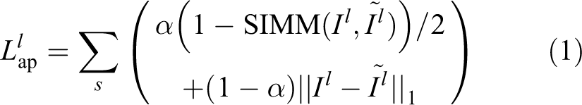
where s denotes the scale, $\text{SIMM}()$ ²⁴ is a function which can measure the structural similarity of two images, and α is the weight parameter to measure the influence between the difference in image appearance and the regularization part.

Considering the fact that depth discontinuities often exist at the image edges, and furthermore, to preserve the sharp details, we also add an edge smoothness to the objective function with the use of the disparity map gradients. The edge-aware smoothness term of the left disparity map is as follows

$L_{\text{Ds}}^l={\displaystyle \sum }_s\left(\begin{array}{c}|\partial D^l/\partial x|\cdot \text{exp}\left(-\Vert \partial x{I}^l{\Vert }_1\right)+\\ |\partial D^l/\partial y|\cdot \text{exp}\left(-\Vert \partial y{I}^l{\Vert }_1\right)\end{array}\right)$

2

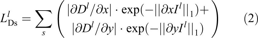
The difference in appearance and the edge-aware smoothness term of the right is similar to that of the left, and we denote them as $L_{\text{ap}}^r$ and $L_{\text{Ds}}^r$ .

The depth CNN produces the left and right disparity maps simultaneously. To improve the estimated disparity maps’ accuracy, we introduce a left-right consistency loss based on the similar geometric constraints, which is the above image reconstruction process just used.

The same image synthesis function including $G_{r\to l}$ and $G_{l\to r}$ are chosen for disparity map reconstruction. The synthesized disparity map from left disparity to the right is $D_{l\to r}=G_{l\to r}\left(D^l,D^r\right)$ , and the synthesized disparity map from right disparity to the left is $D_{r\to l}=G_{r\to l}\left(D^r,D^l\right)$ , and the left-right consistency loss of the stereo image pair $L_{l-r}$ can be formulated as

$L_{l-r}=\sqrt{{\left(D_{l\to r}-D_{r\to l}\right)}^2}$

3

The final loss function of depth CNN becomes

$L_{\text{depth}}={\lambda }_1\left(L_{\text{ap}}^l+L_{\text{ap}}^r\right)+{\lambda }_2\left(L_{\text{Ds}}^l+L_{\text{Ds}}^r\right)+{\lambda }_3{L}_{l-r}$

4

where ${\lambda }_1$ , ${\lambda }_2$ and ${\lambda }_3$ are the weight parameters.

Camera pose prediction

The loss for the pose CNN is constructed according to the temporal photometric error between stereo videos. The left and right monocular image sequences of the stereo video are considered, respectively. The supervisory signal of the pose CNN comes from image synthesis, and the scene depth and camera pose are essential to any loss function of our CNNs. Thus, we train the depth and pose CNN simultaneously and used them separately.

During training, stereo images sequences, which are set at a length of five frames, are selected as the training sample. The temporal photometric loss can be calculated from the stereo videos. Similar to the depth CNN, the projective photometric error of two consecutive images is employed instead of ground truth to construct the loss function. During testing, we fix the parameters of the pose CNN to predict the camera’s 6-DoF transformation.

The left image sequence is denoted as $\left(I_1^l,I_2^l,I_3^l,I_4^l,I_5^l\right)$ . The middle image of this sequence $I_3^l$ is selected as the target frame $I_t^l$ , and the rest frames of this sequence are the source frames.

We synthesize the left target frame $\stackrel{\sim }{I_t^l}$ from the source frames $I_n^l\left(n=1,2,4,5\right)$ based on the geometric constraints $\stackrel{\sim }{I_t^l}=K{T}_{s\to t}{D}_t^l{K}^{-1}{I}_n^l$ , where K is the camera intrinsic matrix, $T_{s\to t}$ is the camera motion from the source frames to the target frame, and $D_t^l$ is the disparity map. The camera motion and the disparity image are generated by the pose and depth CNNs, respectively. The architecture of camera motion prediction is shown in Figure 3. From Figure 3, we can see that depth estimation and pose prediction are two complementary processes. The loss functions of the depth and pose CNNs all require disparity maps and the camera motions to synthesize the images. Hence, we cannot compute only one monocular image sequence of the stereo video.

Figure 3.

Architecture of the camera motion prediction process. It consists of disparity maps generated by depth CNN and the camera motion from source frames to the target frame generated by the pose CNN. The input image sequence including five frames, and the target frame is the third frame of the sequence. CNN: convolutional neural network.

The loss function of the pose CNN is similar to that of the depth CNN. The difference in frame appearance between the target and source frames of the left sequence is as follows

$L_{f\_\text{ap}}^l={\displaystyle \sum }_s\left(\begin{array}{c}\beta \left(1-S\left(I_t^l,\stackrel{\sim }{I_t^l}\right)\right)/2\\ +\left(1-\beta \right)\Vert I_t^l-{\stackrel{\sim }{I_t^l}\Vert }_1\end{array}\right)$

5

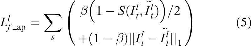
where β is a weight parameter.

The difference in frame appearance of the right sequence is similar to that of the left sequence, and we denote it as $L_{f\_\text{ap}}^r$ .

The final loss function of the pose CNN becomes

$L_{\text{pose}}=L_{f\_\text{ap}}^l+L_{f\_\text{ap}}^r$

6

The loss function for the static scene combines the spatial loss which comes from the depth CNN and the temporal loss which comes from the pose CNN together. Previous approaches such as SfMLearner ¹² and GeoNet ²² used monocular videos as input to train the networks, even though we use stereo videos as input to learn the networks’ parameters, there is no essential distinction between our method and previous approaches. Hence, the improvement in the camera motion prediction compared with previous methods is mainly attributed to the high-precision depth map.

In addition, the reason for the five-frame structure is to compare with previous algorithms. The most famous model, monocular ORB-SLAM, ² has two variants which are full ORB-SLAM and short ORB-SLAM. Full ORB-SLAM uses all frames of the dataset to estimate the camera motion. Short ORB-SLAM uses 5-frame snippets for estimation. The depth and pose CNNs use iterative calculation so that a training sample can only be composed of several frames. To compare our model with short ORB-SLAM, the length of each training sample is five, and the same structure is set by previous deep models. ^22,25

Dynamic object localization

Motion is a fundamental property of any scene. Optical flow reflects the motion of two-dimensional (2D) pixels and scene flow reflects the motion of 3D points in a scene in practice. The scene motion can be obtained through the optical flow between the consecutive frames of a video. The projected 2D images corresponding to 3D scenes in practice comprise two parts: the static structure which determined by the depth image and camera motion, the dynamic objects mainly determined by the relative motion between the objects and the camera. The purpose of optical flow is to compute the 2D image change which is caused by the relative motion. However, it is hard to obtain the desired results which are determined by two variables.

The above depth and pose CNNs achieved the basic spatial geometric information of a scene, but they treat dynamic objects as static views. Moreover, possible occlusions and outliers exist in the stereo image pairs, or the monocular image sequences affect the accuracy of the method inevitably. To solve the above problems, we propose the flow CNN to establish a direct corresponding relationship between an image and the optical flow map.

Optical flow can fully exploit the unconstrained motion, while scene depth and camera motion can develop the fundamental geometric structure of the static scene. This phenomenon enables us to make full use of the combination of the depth CNN, the pose CNN and the flow CNN. The input data of our flow CNN is composed of the original stereo videos and the results which are generated by the depth and pose CNNs. Therefore, 3D scene perception of the static scene gives the flow CNN a good beginning.

The proposed framework is a two-stage course. The first stage trains the depth and pose CNNs, and then fixes the parameters of these two networks for the next stage. The second stage only trains the flow CNN. As a result, the flow CNN only learning the residual flow which is solely caused by the dynamic objects or outliers of the static scene. We also train the flow CNN without the fixed depth and pose CNNs, but the results are inferior to the results of the two-stage strategy.

As illustrated in Figure 4, our flow CNN takes advantage of the output from the static scene synthesis and learns the corresponding optical flow fields. The final full optical flow consists of the static and residual optical flow. The key component of the flow CNN is a differentiable optical flow renderer which reconstructs the optical flow field. We denote $\left(I_1^l,I_2^l,I_3^l\right)$ as the left image sequence with the second frame $I_2^l$ as the target frame $I_t^l$ , and the rest of this image sequence are the source frames. For static scenes, the static optical flow can be calculated by the corresponding scene depth and camera motion, which are obtained from the depth and pose CNNs. The static optical flow can be computed as follows

$\begin{array}{c}Flo{w}_{t\to s}^{\text{rigid}}=C\left(D_t,T_{t\to s},K\right)\\ Flo{w}_{s\to t}^{\text{rigid}}=C\left(D_s,T_{s\to t},K\right)\end{array}$

7

Figure 4.

Architecture of our flow CNN’s loss function. It consists of optical flow map synthesis error for estimating the optical flow and a left-right consistency part for checking the quality of the synthesized optical flow maps. CNN: convolutional neural network.

where D_t and D_s are the disparity maps corresponding to the target and source images, respectively, $T_{t\to s}$ is the camera motion from the target frame to the source frame, $T_{s\to t}$ is the camera motion from the source frames to the target frame. They are obtained by the depth and pose CNNs, respectively. $C\left(\cdot ,\cdot \right)$ is a computing function.

Based on the static optical flow, we can reconstruct the target frames from the source frames and vice versa, and the formulas are as follows

$\begin{array}{c}{I}_{\text{rigid}\_t}^l=F\left(I_s^l,Flo{w}_{t\to s}^{\text{rigid}}\right)\\ I_{\text{rigid}\_s}^l=F\left(I_t^l,Flo{w}_{s\to t}^{\text{rigid}}\right)\end{array}$

8

where $F\left(\cdot ,\cdot \right)$ is the image synthesis function, $t\to s$ means from target frame to source frame and $s\to t$ means from source frames to target frames.

Then, we use the original image sequence and the synthesized image sequence $I_{f\_t}^l$ , $I_{f\_s}^l$ as the flow CNN’s input data. This strategy makes full use of the static scene geometric constraints, which we have already completed in previous CNNs actually. It gives us a good start for the flow CNN, so the flow CNN can localize dynamic objects through the residual optical flow with more concentration.

The flow CNN generates residual optical flow $Flo{w}_{t\to s}^{\text{res}}$ and $Flo{w}_{s\to t}^{\text{res}}$ , while the static optical flow is calculated by the depth image and the corresponding camera motion, so the full optical flow of the left image sequence is the summation of them

$\begin{array}{c}Flo{w}_{t\to s}^{\text{full}}=Flo{w}_{t\to s}^{\text{rigid}}+Flo{w}_{t\to s}^{\text{res}}\\ Flo{w}_{s\to t}^{\text{full}}=Flo{w}_{s\to t}^{\text{rigid}}+Flo{w}_{s\to t}^{\text{res}}\end{array}$

9

The supervisory signal of our flow CNN is based upon the difference between the synthesized frames and the input frames. The synthesized frames are reconstructed by the full optical flow, therefore we use the geometric constraints of the static scene and the dynamic objects’ information to construct our supervisory signal. Similar to formula (8), the synthesized frames from the full optical flow are as follows

$\begin{array}{c}{I}_{\text{full}\_t}^l=F\left(I_s^l,Flo{w}_{t\to s}^{\text{full}}\right)\\ I_{\text{full}\_s}^l=F\left(I_t^l,Flo{w}_{s\to t}^{\text{full}}\right)\end{array}$

10

The error difference between the input and synthesized image sequences is

$L_{\text{flow}}^l={\displaystyle \sum }_s\left(\begin{array}{c}\gamma \left(1-S\left(I^l,I_{\text{full}}^l\right)\right)/2\\ +\left(1-\gamma \right)\Vert I^l-I_{\text{full}}^l{\Vert }_1\end{array}\right)$

11

where I^l means the left original input image sequence $\left(I_1^l,I_2^l,I_3^l\right)$ , $I_{\text{full}}^l$ means the left synthesized image sequence constituted of $I_{\text{full}\_t}^l$ , $I_{\text{full}\_s}^l$ , $\gamma$ is a weight parameter.

A training sample of the flow CNN consists of the stereo image sequence, so the loss function of the right image sequence is similar to $L_{\text{flow}}^l$ , and we denote it as $L_{\text{flow}}^r$ . Similar to formula (2), we compute the smoothness loss of the optical flow for the left and right image sequences. They are denoted as $L_{\text{Df}}^l$ , $L_{\text{Df}}^r$ .

Until now, the depth pose CNNs take advantage of the image synthesis to construct the supervisory signal for the static scene, with the flow CNN using the view synthesis as a supervisory signal for dynamic objects. In addition, we design a left-right consistency as part of the loss function for the static scene. However, this loss part does not consider the moving regions or outliers of the image. To mitigate the adverse impact caused by the dynamic objects, we proposed a forward-backward consistency loss part which is based upon the full optical flow.

Only the target frames are used to design the forward-backward consistency check. The full optical flow of the target frame includes the rigid optical flow corresponding to the static scene and the residual optical flow corresponding to dynamic objects. Therefore, the full optical flow is used to reconstruct the optical flow fields of the left and right image sequences, respectively. These synthesized optical flow fields take into consideration all of the scene information so that the final model can reduce the impact of moving objects and occlusion effectively.

The image synthesis functions which come from formula (10) are selected to construct the forward-backward loss function. We use $Flo{w}_{t\to s}^{\text{full}}$ and $Flo{w}_{s\to t}^{\text{full}}$ to reconstruct the corresponding optical flow fields as follows

$\stackrel{\sim }{\begin{array}{c}\stackrel{\sim }{Flo{w}_{s\to t}^{\text{full}}}=F\left(Flo{w}_{s\to t}^{\text{full}},Flo{w}_{s\to t}^{\text{full}}\right)\\ \stackrel{\sim }{Flo{w}_{t\to s}^{\text{full}}}=F\left(Flo{w}_{t\to s}^{\text{full}},Flo{w}_{s\to t}^{\text{full}}\right)\end{array}}$

12

Then, left and right forward-backward consistency loss can be defined based on the formula as follows

$\begin{array}{c}{L}_{f\_b}={|\stackrel{\sim }{Flo{w}_{s\to t}^{\text{full}}}-Flo{w}_{s\to t}^{\text{full}}|}_1+\\ {|\stackrel{\sim }{Flo{w}_{t\to s}^{\text{full}}}-Flo{w}_{t\to s}^{\text{full}}|}_1\end{array}$

13

With reference to formula (10), the synthesized optical flow field is reconstructed by the full optical flow, which includes the information of dynamic objects or occlusion. Therefore, the forward-backward consistency loss can mitigate the influence of non-static motion and occlusions. The final loss function of our flow CNN is as follows

$L_{\text{flow}}={\mu }_1\left(L_{\text{flow}}^l+L_{\text{flow}}^r\right)+{\mu }_2\left(L_{\text{Df}}^l+L_{\text{Df}}^r\right)+{\mu }_3\left(L_{f\_b}^l+L_{f\_b}^r\right)$

14

where ${\mu }_1$ , ${\mu }_2$ and ${\mu }_3$ are weight parameters.

The objective function

Monocular video has two inevitable defects. The first defect is the unknown camera motion, and the other is the ambiguity in scale. The use of stereo video during training takes advantage of both spatial and temporal geometric information to solve both of these problems. In the test time, our model can estimate the scene depth, predict camera motion and localize dynamic objects with only monocular video as input. The key supervisory signal comes from the image synthesis error while the smoothness of the appearance acts as an auxiliary loss. Furthermore, the left-right and forward-backward consistency checks are used to encourage consistency in the spatial and temporal geometric information.

The final objective function in our model becomes

$L={\sigma }_1{L}_{\text{depth}}+{\sigma }_2{L}_{\text{pose}}+{\sigma }_3{L}_{\text{flow}}$

15

where ${\sigma }_1$ , ${\sigma }_2$ and ${\sigma }_3$ are weight parameters.

Experiments

Here, we evaluate our unsupervised framework for depth estimation, camera motion prediction and dynamic objects localization from monocular video. The KITTI ²⁶ and Cityscapes ²⁷ datasets are used for training, testing and evaluating the generalization ability. Furthermore, we conduct an ablation study on the proposed method to discuss the effects of the left-right and forward-backward consistency checks. We use the same split with ⁵ to evaluate the depth estimation performance. The KITTI odometry dataset is used to evaluate the camera motion, the KITTI odometry and flow2015 datasets are used to evaluate the optical flow’s performance.

Network architecture and detail

For monocular depth estimation and dynamic objects localization, we construct an encoder-decoder architecture. Our model is mainly based on ResNet50. ²⁸ The exponential linear unit is used as activation function except for the decision layers. For camera motion prediction, an encoder architecture mainly based on modules that consist of convolutional layers and the rectified linear unit layers are chosen to compute the camera pose.

Our depth and flow CNNs use the same architecture. For static region perception, these CNNs contain about 60 million=trainable parameters; for dynamic objects localization, the CNN contains about 30 million trainable parameters. In the two stages, we use a single NVIDIA GTX 1080Ti GPU with 600 and 800 thousand iterations, respectively. The training time of static region perception is about 27 h, then we fix the depth and flow CNNs’ parameters to train the flow CNN solely, the training time of this stage is 17 h. During training we use the Adam algorithm to optimize the network; the initial learning rate is 0.0002 for the first half of the iterations, and we halving it until the end. The Adam optimizer’s parameters are set as ${\beta }_1=0.9,{\beta }_2=0.999,ϵ={10}^{-8}.$

Monocular depth estimation

For depth estimation, we chose the KITTI raw dataset for training and testing. It is captured by an autonomous driving platform around the mid-size city of Karlsruhe. It contains 42,382 rectified stereo images that are 1243 × 375 pixels in size, captured from 61 scenes.

The testing split of Eigen et al. ⁵ is used for evaluating. During the training process, all visual-like frames are excluded from the testing scenes, which are the same as Zhou et al. ¹² Unlike previous unsupervised systems, our method uses stereo image sequences for training but only monocular image sequences are required for testing. Thus, we capture 35,621 stereo images pairs from the ‘city’, ‘residual’ and ‘road’ categories to generate the stereo image sequences for training (Zhou et al.’s article used about 71,242 monocular images to construct the training dataset). The length of each sequence is three. At last, we resize the stereo images to 416 × 128 pixels in size during training and the output of our model is also 416 × 128 pixels in size.

Table 1 provides the evaluated performance on the same 697 images as Eigen’s test split dataset. We use the same performance measures as previous methods to judge the depth estimation accuracy.

Table 1.

Monocular depth estimation results on the KITTI and Cityscapes datasets.

Method	Super-vision	Lower is better				Higher is better
		Abs Rel	Sq Rel	RMSE	RMSE log10	δ ≤ 1.25	δ ≤ 1.252	δ ≤ 1.253
Eigen 1	Yes	0.214	1.605	6.563	0.292	0.673	0.884	0.957
Eigen 2	Yes	0.203	1.548	6.307	0.282	0.702	0.890	0.958
Liu	Yes	0.202	1.614	6.523	0.275	0.678	0.895	0.965
Garg	No	0.177	1.169	5.285	0.282	0.727	0.896	0.958
Zhou	No	0.208	1.768	6.856	0.283	0.678	0.885	0.957
Li’s	No	0.183	1.730	6.570	0.268	–	–	–
Geonet	No	0.155	1.296	5.875	0.233	0.793	0.931	0.973
Wang’s	No	0.151	1.257	5.583	0.228	0.810	0.936	0.974
Zhang’s	No	0.144	1.391	5.869	0.241	0.803	0.928	0.969
Ours (K)	No	0.139	1.297	5.879	0.223	0.827	0.936	0.979
Ours (C)	No	0.154	1.545	5.926	0.236	0.812	0.912	0.958
Ours (C + K)	No	0.126	1.122	5.301	0.204	0.845	0.944	0.983

K: KITTI dataset; C: Cityscapes dataset; C + K: Cityscapes + KITTI datasets.

As shown in Table 1, the comparable algorithms trained on the KITTI dataset include more than one data structure, such as stereo image pairs (Garg et al. ¹⁰ ), monocular videos (Zhou et al, ¹² GeoNet, ²² Wang et al.’s ²⁹ ) and binocular videos (Li et al.’s, ¹⁶ Zhang et al.’s ¹⁷ ). Some qualitative results are visualized in Figure 5.

Figure 5.

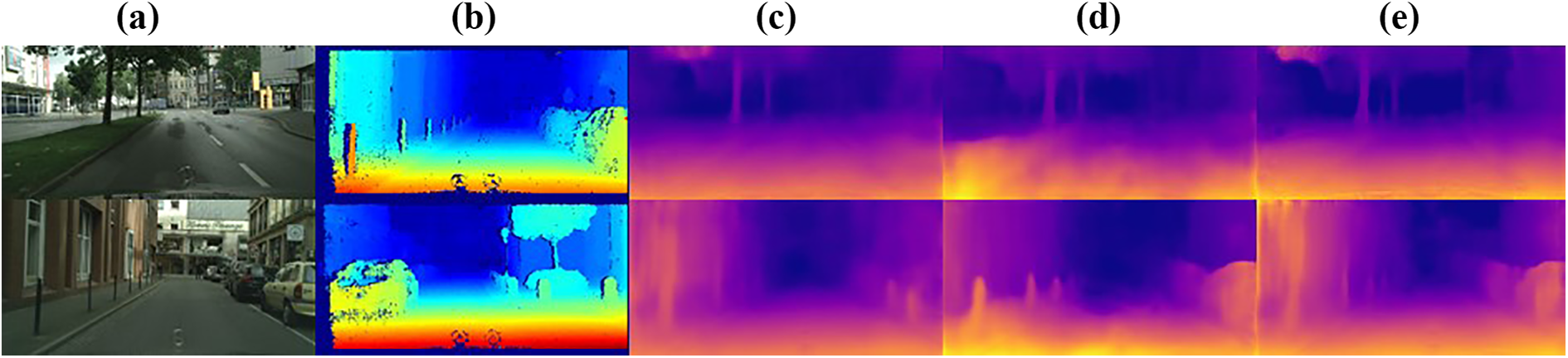
Disparity images of (a) input image, (b) GT, (c) R. Garg, (d) GeoNet, and (e) ours.

As shown in Figure 5, the input images are selected from the KITTI raw dataset randomly. Quantitative results and visualization comparison show that our model is effective, especially in areas with a thinner structure such as a tree trunk. In addition, to evaluate the model’s generalization ability, we apply the model that trained on the KITTI + Cityscapes datasets to the testing set.

The Cityscapes dataset ²⁷ is a benchmark suite for pixel-wise depth estimation and semantic labelling that contains large stereo videos collected from 50 different cities in Germany. All stereo images of the Cityscapes dataset are selected for training.

The monocular depth results of the model trained on the KITTI + Cityscapes datasets significantly outperform the previous unsupervised methods. ^12,22 The quantitative comparison of experiments with previous methods is made in Table 1. The visualized results which are trained on the KITTI dataset (K), ²⁶ Cityscapes dataset (C) ²⁷ and KITTI + Cityscapes datasets (K + C) ^26,27 are shown in Figure 6.

Figure 6.

Disparity images between the proposed model that trained on the KITTI dataset, the Cityscapes dataset and the KITTI and Cityscapes datasets jointly: (a) input image, (b) GT, (c) K²⁷, (d) C²⁸, and (e) K+C^–28.

In addition, obtaining 3D geometric information from a 2D image has a significant application in autonomous robotic applications and self-driving technology. For example, Tesla is trying to use cameras instead of Laser radar for depth estimation. To test the inference performance of our model with images in the actual scene, we used a cell phone camera to collect some data ourselves as input to the network.

As shown in Figure 7, we collected some data as input to the depth CNN to estimate its depth information. Cars, cyclists and some thin structures such as trees are visualized precisely. Moreover, only a single image is required for inference, and it is an impossible task for visual SLAM. The results show the efficiency of our proposed model. We believe this technology will be used for self-driving platforms in the future.

Figure 7.

(a and b) Results of depth estimation.

Camera motion prediction

To evaluate the pose CNN’s performance, we used the KITTI odometry dataset ²⁶ for training and testing. This dataset consists of 22 stereo image sequences but only 00-10 sequences with ground truth trajectories. Considering only the sequences 00-10 of the KITTI odometry dataset with ground truth trajectories, sequences 00-08 are used for training and sequences 09-10 are used for testing. Some other models such as SfMLearner ¹² and UnDeepVO ¹⁶ use the same splitting. In the process of training, the length of a training sequence is set to be five and the size of each frame captured from the stereo video is resized to 416 $\times$ 128 pixels. During testing, monocular video is used to evaluate the performance, the sequence length and the frame size are the same as those of the training process.

We compared the camera motion prediction of our model with two monocular ORB-SLAMs ^2,30 : The full ORB-SLAM uses an entire sequence as input, and the short ORB-SLAM only takes five frames as a testing sample. We also compare our method with several representative unsupervised deep learning models ^12,22 to measure the effect of our method. All results are evaluated with five frames. The absolute trajectory error ² is chosen as the metric. Quantitative results are shown in Table 2.

Table 2.

ATE on the KITTI 2015 odometry dataset.

Method	Seq. 09	Seq. 10
ORB-SLAM (full)	0.014 ± 0.008	0.012 ± 0.011
ORB-SLAM (short)	0.064 ± 0.141	0.064 ± 0.130
SfMLearner	0.021 ± 0.017	0.020 ± 0.015
Geonet	0.012 ± 0.007	0.012 ± 0.009
Ours	0.010 ± 0.005	0.012 ± 0.007

ATE: absolute trajectory error; ORB-SLAM: ORB-simultaneous localization and mapping systems.

Figure 8 gives the relative camera position of the camera coordinate system. Five consecutive frames are used as an input sample to the networks during training and testing stages. The pose CNN outputs five consecutive camera poses that correspond to the input frames. Each five-camera pose sequence uses the first frame as the origin of coordinates of this five frames sequence. We compared our methods with ground truth, Geonet and SfMLeaner. The first column of the figure shows the relative camera motion in the x-axis and z-axis, respectively, for image sequence 09, and the second column shows that for image sequence 10.

Figure 8.

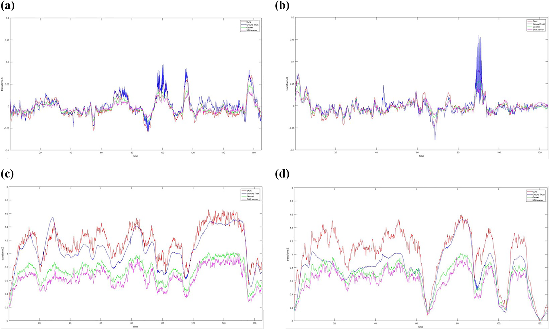
(a to d) The relative camera trajectory.

As shown in Table 2, better performance is achieved by our model in camera motion prediction than other monocular methods even without scale pre-processing and post-processing. In Figure 8, the relative camera pose of the presented model is closer to the truth trajectories. In particular, for image sequence 09, it is almost the same as ground truth. Moreover, we attempt to plot the absolute camera trajectories of our model and several compared methods, but the results cannot give an intuitive description of the camera motion, as shown in Figure 9. We think the reason is that each relative camera pose has a minor error compared with the ground truth, the error of the absolute trajectory increase with repeatedly inner products. Consequently, we transform the absolute trajectory of the ground truth to five relative camera poses to show the performances of our model and some compared methods (as shown in Figure 8).

Figure 9.

(a and b) Absolute camera trajectory.

The accuracy of the absolute camera trajectory of our model is inferior to ORB-SLAM. The phenomenon is caused by several reasons such as our neural networks use mini-batch frames as input to train the model, and the lack of relocalization and loop closing stages. Until now, for absolute camera trajectory prediction, deep CNNs are still falling behand SLAM algorithms.

Dynamic object localization

We choose the KITTI raw datasets for training, and the KITTI flow2015 dataset is chosen for evaluation of the dynamic object localization. These datasets consist of 200 training and testing scenes, respectively. In the testing process, only monocular video is required. The corresponding flow non-occlusion and occlusion datasets are also needed.

Optical flow represents the motion information of relative pixels. Because of the pixel-wise characteristics, it has become an important technology for non-rigid pixel localization. General optical flow techniques compute the dynamic objects without fully utilizing the geometric constraints of the static regions, which we have completed in advance. The depth and pose CNNs compute the 3D scene information of the static region, it gives a good starting point for dynamic object localization. Based on the results of these two CNNs, we fix the parameters of the depth and pose CNNs, then we train the flow CNN (full-flow CNN) to localize the dynamic objects and through the scene optical flow. To verify the influence of static regions, we also train the flow CNN (direct-flow CNN) directly without any information on the depth and pose CNNs. Figure 10 gives the results of the two flow CNN models. The optical flow results which are generated by the direct-flow and direct-flow CNNs are direct and residual results, respectively. As shown in Figure 10, the residual results give a more detailed structure of the optical flow especially in the edge regions. However, in this view synthesis process, some problems such as occlusions may be unavoidable. To show the effectiveness of our forward-backward consistency in mitigating these impacts, we give the visualization results in Figure 11 with quantitative results shown in Table 3.

Figure 10.

Comparison of optical flow in (b) GT, (c) the direct method with the raw stereo image sequences as input, and (d) the residual method with the raw stereo image sequences and the results of the static region as (a) input. GT: ground truth.

Figure 11.

Comparison of optical flow in GT, results without and with forward-backward consistencies: (a) input image, (b) GT, (c) result without f-b, and (d) result with f-b. GT: ground truth.

Table 3.

Average EPE on the KITTI flow 2015 dataset over NOC and ALL.

Method	Dataset	NOC	ALL
FlowNet	C + S	8.12	14.19
FlowNet2	C + T	4.93	10.06
GeoNet	K	8.05	10.81
Direct result	K	8.23	12.06
Result without f-b	K	7.49	11.25
Final result	K	6.45	9.87

NOC: non-occluded regions; ALL: overall regions.

Figure 11 provides several examples of visual comparison between results with and without forward-backward consistency. These comparisons show that our forward-backward consistency improves the effectiveness of the algorithm. Even though this forward-backward consistency has no significant improvement in visual effect, we can get quantitative comparisons in Table 3.

To measure the model’s performance, we compare our dynamic object localization results with GeoNet. ²² The end-point error is used over non-occluded regions and overall regions for quantitative comparisons. The same KITTI stereo/flow split as GeoNet is used to achieve fair qualitative and quantitative comparisons (as shown in Table 3). The visual results are shown in Figure 12.

Figure 12.

Comparison of optical flow in (b) GT, (c) GeoNet and (d) ours. The (a) input images and ground truth are captured from the KITTI stereo2015 datasets. GT: ground truth.

As a pixel-wise strategy, optical flow is a crucial strategy to calculate the geometric relationship of pixels in non-static regions. In this part, we establish the corresponding relationship between scene flow and optical flow, then use the flow CNN to localize the dynamic objects through the optical flow. Even though the visual effect is not obvious, dynamic object localization is a challenging problem and we provide an important method for this topic.

Comparison of real-time performance

In robotic and autonomous vehicle applications, real-time performance is crucial. We use one of the most famous real-time methods which is ORB-SLAM ² as a baseline to measure our model’s real-time performance. Moreover, we also compare it with a deep CNN model. ²² ORB-SLAM includes multiple stages such as feature extracting, mapping and bundle adjustment. Only the depth information of each feature point is generated by ORB-SLAM system, so we use the processing time of the local mapping as depth estimation stage.

During navigation process, the depth information of a feature point is similar to that of an image pixel. The processes of map point creation and local bundle adjustment are 66.79 and 296.08 ms, the processing time of GeoNet and our model are 15 and 25 ms, respectively. Even though only the map point creation stage is used for comparison, our model is faster than that stage.

The stage of camera motion prediction is corresponding to the tracking stage of ORB-SLAM, which is composed of ORB extraction, pose estimation and track local map. The total time of the tracking stage is 30.57 ms and our model only uses 4.5 ms to predict the camera pose. Only considering the pose of a single point, ORB extraction and pose estimation takes 14.48 ms, which is slower than our model.

However, during depth estimation and camera motion prediction stages, our model is slower than GeoNet, the reasons are as follows: (1) GeoNet uses a single TitanXP GPU for testing and the GPU of ours is GTX 1080Ti, which is behind TitanXP and (2) to improve the model’s accuracy, we use stereo videos as input which make the configuration is more complex than GeoNet. Though our model is slower than GeoNet, the proposed model can meet the real-time demand of robotics and autonomous vehicle application.

Conclusion

This article proposed an unsupervised learning algorithm to estimate the scene depth, camera motion and optical flow. The supervisory signal is constructed based on various formats of multi-view image synthesis. Stereo videos are used as input to the model to learn the CNNs’ parameters. In the inference stage, we fix the learned parameters, and only monocular videos are required. Compared to other unsupervised approaches and several supervised methods, the experiment results indicate that our method outperforms the previous approaches. Understood as key problems in 3D scene perception, depth estimation, camera motion prediction and dynamic objects localization are solved by the proposed framework. Therefore, the presented method is close to solving the fundamental problems of 3D scene perception through an unsupervised strategy.

There are several subjects for future study. Firstly, the training dataset gives the camera intrinsic matrix, which constrains the use of random videos without camera calibration previously. Secondly, to take advantage of the results of the static region, we have to use a two-stage process to localize the dynamics or occlusion. Lastly, the results of dynamic object localization are fuzzy through the optical flow.

In view of the above disadvantages, in the future, we would like to construct a strict end-to-end framework to localize the dynamic objects with great accuracy and extend our model so that it can learn with random videos.