Sage Journals: Discover world-class research

Abstract

Path planning of lunar robots is the guarantee that lunar robots can complete tasks safely and accurately. Aiming at the shortest path and the least energy consumption, an adaptive potential field ant colony algorithm suitable for path planning of lunar robot is proposed to solve the problems of slow convergence speed and easy to fall into local optimum of ant colony algorithm. This algorithm combines the artificial potential field method with ant colony algorithm, introduces the inducement heuristic factor, and adjusts the state transition rule of the ant colony algorithm dynamically, so that the algorithm has higher global search ability and faster convergence speed. After getting the planned path, a dynamic obstacle avoidance strategy is designed according to the predictable and unpredictable obstacles. Especially a geometric method based on moving route is used to detect the unpredictable obstacles and realize the avoidance of dynamic obstacles. The experimental results show that the improved adaptive potential field ant colony algorithm has higher global search ability and faster convergence speed. The designed obstacle avoidance strategy can effectively judge whether there will be collision and take obstacle avoidance measures.

Keywords

Lunar robot ant colony algorithm artificial potential field dynamic obstacle avoidance

Introduction

There are abundant unexploited resources on the moon. Many countries are promoting the lunar exploration project actively. The lunar robot is an indispensable part of the lunar exploration project, and the path planning is the guarantee for the lunar robot to complete its tasks safely and accurately in the lunar environment. The goal of path planning is to enable the robot to find an optimal path from the start point to the destination. Limited by the energy carried by lunar robot, seeking the shortest path is the optimal goal of the path planning algorithm.

In various traffic planning problems, route planning has been widely studied and discussed. These algorithms mainly include A* algorithm, simulated annealing algorithm, genetic algorithm, differential evolution algorithm, particle swarm optimization algorithm, ant colony algorithm, and so on. Those algorithms have been widely used in engineering practice. A* algorithm¹ determines the next path grid step-by-step by comparing eight adjacent heuristic function values of the current path grid. In the simulated annealing algorithm,² by controlling the temperature parameter T and using the Metropolis criterion, the attenuation function is used to change the temperature t to minimize the objective function and determine the next target point. Genetic algorithm³ uses crossover and mutation to determine the next target point and to achieve the optimal path selection. The differential evolution algorithm based on the evolution idea of genetic algorithm⁴ solves the shortest path problem through hybridization, mutation, and selection. Particle swarm optimization algorithm⁵ is to know the next iteration position of particles using the current position, global extremum, and single extremum. Ant colony algorithm⁶ is a kind of bionic algorithm that simulates the way ants search for food in nature. The basic idea is to find the shortest path according to the concentration of pheromone left by ants. In these methods, with the increasing complexity of obstacles, the convergence speed of genetic algorithm, simulated annealing algorithm,⁷ A* algorithm,⁸ and differential evolution algorithm⁹ will slow down. The robustness of particle swarm optimization algorithm is poor slightly, and the optimal solution depends on initialization. Ant colony algorithm has advantages in positive feedback, robustness, and so on. It is easy to combine with various heuristic algorithms to speed up convergence speed and reduce resource consumption when the algorithm is running, so it has been widely used in robot path planning.

Considering the energy consumption and dynamic obstacle avoidance, the grid method is used to process the simulated map data. Then the adaptive potential field ant colony algorithm is used to do the path planning. This method adjusts the heuristic function dynamically by introducing the inducing heuristic factor, so as to improve the global optimization ability and accelerate the convergence speed. The proposed adaptive potential field ant colony algorithm is called A-APFACO. In addition, predictable and unpredictable obstacle avoidance strategies are also considered. Therefore, we propose a geometric method for detecting dynamic obstacles.

The organizational structure of the article is as follows. The second section describes the related work. The third section mainly describes the environment modeling based on grid map method and an A-APFACO. The fourth section describes the dynamic obstacle avoidance strategy. The fifth section describes the experiments and results. The sixth section summarizes the whole paper.

Related work

Ant colony algorithm has been proved as good performance in path planning. However, it still has unavoidable shortcomings, such as long search time, slow convergence speed, and falling into local optimum easily. To improve the performance of ant colony algorithm, many researchers proposed improvement schemes. Stutzle and Hoos¹⁰ proposed the maximum and minimum ant system algorithm, which introduced the definite maximum and minimum trajectories into the path. By constraining the maximum and minimum trajectories, the problem of stagnation was solved. Liu et al.¹¹ proposed an algorithm for path planning of mobile robots. This algorithm uses grid method to simulate the environment, and in the process of global optimization, pheromone diffusion and geometric local optimization are combined to accelerate the convergence speed of ant colony algorithm. Cheng et al.¹² combined simulated annealing algorithm with ant colony algorithm to speed-up pheromone updating. Long et al.¹³ combined the evaluation function of A* algorithm with ant colony algorithm to improve the speed of convergence and the smooth of planned path. As can be seen, the methods mentioned in the literature^10

–13 have improved the state transition rule and accelerated the convergence speed of ant colony algorithm, but they cannot adjust the state transition rule adaptively, which made the algorithm easily fall into local optimum. Akka and Khaber¹⁴ used new pheromone updating rule to adjust the evaporation rate dynamically, accelerated convergence speed, and expanded the search space of ant colony algorithm. Yang et al.¹⁵ proposed a double-deck ant colony optimization algorithm, which consisted of a parallel elite ant colony optimization algorithm and smoothness optimization algorithm. It was mainly used for autonomous navigation of robots. This method can generate better collision-free paths effectively and consistently. However, the method mentioned in the literature^14,15 can only be applied to fixed environment, which means the distribution of obstacles is fixed. Once the environment changes, the parameters of algorithm need to be readjusted.

Dynamic obstacle avoidance problem is also a key point for robot. Many scholars have proposed solutions. Aiming at distributed robots, Javier et al.¹⁶ proposed a method of combining constrained nonlinear optimization with consistency to avoid static and dynamic obstacles. However, this method can only be applied to predictable dynamic obstacle, it is invalidation for unpredictable obstacle. Hu et al.¹⁷ used global routes to construct centerlines, generated a set of candidate paths in the s–q coordinate system, and converted them into Cartesian coordinates. The optimal path was selected by considering the total energy consumption. Wang et al.¹⁸ proposed a probabilistic model for three kinds of robot dynamic obstacle avoidance based on Markov decision algorithm in uncertain dynamic environment. With PRISM software, the minimum time and energy consumption of each obstacle avoidance strategy were obtained, and the optimal obstacle avoidance strategy under different conditions was determined. However, only a single form of dynamic obstacle avoidance is considered in the studies by Hu et al.¹⁷ and Wang et al.,¹⁸ just codirectional motion is considered in the study by Hu et al.,¹⁷ while intersecting motion is considered in the study by Wang et al.¹⁸ Sun et al.¹⁹ proposed a new artificial potential field algorithm danger index artificial potential field (DIAPF) based on hazard index, which considered the relative distance as well as the relative velocity between the robot and the moving obstacle. However, when encountering dynamic obstacle, this method needs to replan the path according to the speed of dynamic obstacle. Wang²⁰ proposed an autonomous obstacle avoidance optimization algorithm. The problem of autonomous obstacle avoidance of unmanned aerial vehicle is transformed into the problem of solving quadratic equation of one variable, and the expected speed and angle are calculated to achieve obstacle avoidance. However, the premise of this method is that the robot and obstacles need to maintain a fixed speed. If the speed changes, it will lead to the failure of obstacle avoidance.

An adaptive potential field ant colony algorithm

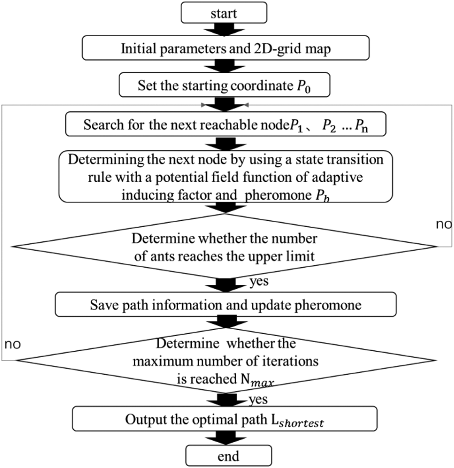
Aiming at the problems of falling into local optimum, slow convergence, and dynamic obstacle avoidance in ant colony algorithm, firstly, we propose an improved potential field ant colony algorithm based on dynamic obstacle avoidance. Then, we improve the heuristic function in the transfer probability based on the ant colony algorithm. Finally, a dynamic transfer strategy, which enables robots to avoid obstacle in dynamic environment, is proposed. The main flowchart is as shown in Figure 1.

Figure 1.

Flowchart of A-APFACO based on dynamic obstacle avoidance strategy.

Environment modeling based on grid method

Considering that, the lunar environment is relatively simple and full of ring mountains and plains. The environment model is simplified to a two-dimensional (2D) grid map, and the moving path of robot is planned in map as shown in Figure 2.

Figure 2.

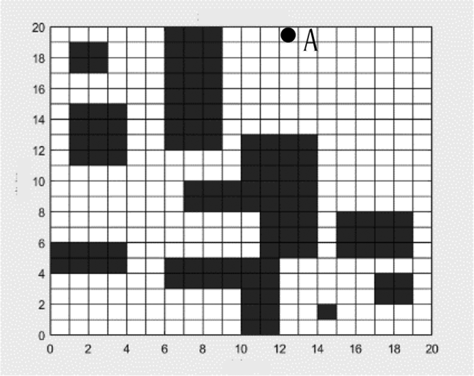
Grid map.

Figure 2 shows a 2D grid map with 20 rows and 20 columns, where black grid represents obstacle and white grid represents accessible space. In the 2D plane, the coordinates of each grid are calculated in the orthogonal reference coordinate XOY. Assuming that the entire grid is marked with integer and their length are equal to the unit length of coordinate, the following coordinate can be obtained as

\{\begin{cases} x_{i} = mod (i, N_{x}) \\ y_{j} = mod (j, N_{y}) \end{cases}

Among them, N_x denotes the number of grids of each row, N_y denotes the number of grids of each column, and mod is the remainder operation. Here, N_x = 20, N_y = 20, the coordinate of point A is x_i = 13, y_j = 19.

Adaptive potential field ant colony algorithm

Ant colony algorithm

Dorigo et al.⁶ proposed an ant colony algorithm (ACO) in 1996, which is a heuristic algorithm for finding the optimal solution. It simulates the foraging behavior of ants. Assume at time t, the ant k chooses the next node according to formula (2)

P_{i j}^{k} (t) = \{\begin{cases} \frac{{(τ_{i j} (t))}^{α} {(η_{i j} (t))}^{β}}{\sum_{s \in {allow}_{k}} {(τ_{i j} (t))}^{α} {(η_{i j} (t))}^{β}} \\ 0 \end{cases}

Here, $P_{i j}^{k} (t)$ denotes the probability of ants moving from point i to point j, $τ_{i j} (t)$ represents the remaining pheromone from point i to the next node, $j \in {allow}_{k}$ denotes the point that has been allowed by ant k, $η_{i j} (t)$ is a heuristic function, and α and β denote the importance of pheromone and heuristic function in the state transition rule, respectively. Heuristic function is defined as

η_{i j} (t) = \frac{1}{d_{i j}}

where d_ij denotes the distance from point i to point j, d_ij is defined as

d_{i j} = \sqrt{{(x_{j} - x_{i})}^{2} + {(y_{j} - y_{i})}^{2}}

The updated pheromone is determined by the volatile pheromone and the pheromone left by ants. The updated formula of pheromone is as follows

τ_{i j} (t + 1) = (1 - ρ) τ_{i j} (t) + \sum_{k = 1}^{m} Δ τ_{i j}^{k}

Here, ρ represents the evaporation rate of pheromone, m is the number of ants, and $Δ τ_{i j} (t)$ represents the pheromone left by ants under the current iteration round, which can be expressed as

Δ τ_{i j}^{k} = \{\begin{cases} \frac{Q}{L_{k}} L_{k} \in shortest path \\ 0 otherwise \end{cases}

Improvement of heuristic function

(1) Improvement of heuristic function based on artificial potential field method.

Artificial potential field method is an effective method to solve the problems of slow convergence caused by blind search in the early stage of the ant colony algorithm. Artificial potential field is a virtual force field exerting on the environment, usually consisting of gravity and repulsion. Let the gravitational function be G(t), which is defined as the relative distance between the robot and the target. The calculation formula is as follows

G (t) = \frac{1}{1 + \sqrt{{(x_{s} - x_{i})}^{2} + {(y_{s} - y_{i})}^{2}}}

Among them, $(x_{i}, y_{i})$ is the coordinate of the current node, $(x_{s}, y_{s})$ is the coordinate of the target point. If the current point is close to the target point, the denominator will be zero. The denominator introduces a constant of 1 to ensure computability. Here, the gravitational function is equivalent to the heuristic function $η_{i j}$ in the original ant colony algorithm. Compared with the formula (3), the gravitational function as the heuristic function only needs to consider the distance between the current node and the end, instead of the location of the next node. That is, the selection of the next node can be directly obtained by the gravitational function, which can speed up the convergence rate.

The repulsion function in the artificial potential field is R(t). The repulsion function takes advantage of the position information of the obstacle. It is defined as a function between the robot and the obstacle. The calculation formula is as follows

R (t) = \{\begin{cases} 1 (x_{i}, y_{j}) is not in the obstacles \\ 0 otherwise \end{cases}

$(x_{i}, y_{j})$ is the coordinate of the node to be moved to, when there is obstacle in this node, R(t) = 0 and the robot will not move to the node. On the contrary, R(t) = 1, it will not affect the calculation of the state transition rule.

After introducing artificial potential field, the heuristic function is as follows

η_{i j} = G (t) R (t)

(2) Improvement of heuristic function based on adaptive inducement heuristic factor.

The heuristic function solves the problem of convergence speed for the original heuristic function in ant colony algorithm, but it is still unable to solve the problem of weak global search ability in the later stage of the algorithm. In this article, iteration is considerate as the negative feedback coefficient to make the pheromone change adaptively, which ensures the consistency between the optimization ability and the convergence speed. We define λ as an adaptive inducing heuristic factor

λ = 0.7 + log (1 + \frac{N_{max} - N}{N_{max}})

Here, N _max and N are the maximum and current number of iterations, respectively. In the prophase, the heuristic factor is more than 1, the heuristic function is dominant, and the heuristic function is strengthened, which leads ants to move in a directional manner. In the anaphase, N becomes larger and the heuristic factor is less than 1. At this time, the heuristic function will be weak and the pheromone will play a main role in the stage, which helps ants to find a new way based on pheromone updating.

Finally, the heuristic function after introducing adaptive inducing heuristic factor is as follows

η_{i j} = λ G (t) R (t)

A-APFACO compared with the maximum and minimum ant colony algorithm proposed in the study by Stutzle and Hoos¹⁰; although the maximum and minimum ant colony algorithm improves the local optimization ability to a certain extent, this article combines the artificial potential field with the ant colony algorithm, which has better convergence and global optimization characteristics. Compared with the ant colony optimization with pheromone diffusion model and geometrical optimization path method (ACO-PDG) algorithm proposed in the study by Liu et al.¹¹, the convergence speed of the algorithm in Liu et al.’s work will be slower in the later stage, and the adaptive heuristic function designed in this article can further accelerate the convergence speed of the algorithm in the later stage.

Adaptive artificial potential field ant colony algorithm

The flowchart of the A-APFACO is as shown in Figure 3. The pseudocode of the adaptive artificial potential field ant colony algorithm is presented in Table 1.

Figure 3.

Flowchart of ant colony algorithm.

Table 1.

Algorithm of A-APFACO.

Algorithm 1. A-APFACO

Robot dynamic obstacle avoidance strategy

Obstacle avoidance strategy

Ant colony algorithm can plan to avoid known static obstacles. However, the dynamic obstacle avoidance between lunar robots should also be considered when a lunar robot cluster appears. Since the scene is set on the surface of the moon, the number of lunar robots is limited at present. Assuming that the number of robots is n, $1 \leq n \leq 3$ , all of these robots obey the control from the same organization.

In the case of dynamic obstacle avoidance, moving obstacle can be divided into predictable obstacle and unpredictable obstacle. Since all lunar robots have path planning, and their moving speed is fixed or known, the collision point is predictable. We define this kind of obstacle avoidance problem as predictable obstacle avoidance. However, if something goes wrong while robot is moving, the obstacle avoidance problem will be unpredictable.

Defining robot R has a set of traveling attributes {direction, action, velocity, priority, interaction}, in which direction is the moving direction of robot, direction = {forward, backward, left, right, left up, left down, right up, right down}. The action is the motion state of the robot, action = {move, stop}. The velocity is the speed of the robot, usually it is a known quantity. The priority is the priority of the robot. According to the number of robots, priority = {1, 2, 3}. The collision state of robots can be defined as interaction = {opposite motion, codirectional motion, intersectional motion}.

Predictable dynamic obstacle avoidance strategy

1. Minimum safe distance.

For multi-robot working environment, collision avoidance rule should be given to enable robots to work cooperatively and improve work efficiency. To avoid collision, the distance between two lunar robots should be greater than the minimum safety distance.

Assuming that the two robots are R ₁ and R ₂, and their current coordinates on the 2D grid map are $(x_{1}, y_{1})$ and $(x_{2}, y_{2})$ . The collision avoidance strategy will be initiated when the distance d between the two robots is less than the minimum safe distance h. ²¹

d = \sqrt{{(x_{1} - x_{2})}^{2} + {(y_{1} - y_{2})}^{2}} < h

2. Obstacle avoidance strategy.

To avoid obstacles, priority-based alternative traffic strategy is adopted in this article.

Let two robots be R ₁ and R ₂ respectively, because obstacles are predictable and their trajectories are known. The obstacle avoidance strategies are as follows:

i. Strategy 1:

If interaction = opposite motion, R ₁ move up and down and R ₂ move up and down on the 2D grid map, R ₁.action = move, R ₂.action = move.

At time t, the distance d between R ₁ and R ₂ is less than h. If R ₁.priority > R ₂.priority, R ₂ judges whether there are obstacles on its left or right side based on the map information.

If bilateral or unilateral obstacle-free, at moment t + 1, R ₂ conducts lateral avoidance. R ₂.direction = left or right. Then R ₂.action = stop until R ₁ passes through. Then R ₂.action = move, R ₂ returns to the original route and continues to drive.

If there are obstacles on both sides, at moment t + 1, R ₂.action = move, R ₂.direction = backward, until R ₂ retreats to the barrier-free area, R ₂.direcrion = left or right, R ₂ executes lateral avoidance, R ₂.action = stop, until R ₁ passes through, R ₂.action = move, R ₂ returns to the original route and continues to drive.

ii. Strategy 2:

If interaction = codirection, R ₁ and R ₂ move up and down from the 2D grid map, R ₁.action = move, R ₂.action = move.

If R ₁ is in front of R ₂, R ₁.velocity > R ₂.velocity, no evasion is required.

If R ₁ is in front of R ₂, R ₁.velocity < R ₂.velocity, R ₁ executes lateral avoidance.

Firstly, R ₂.action = stop. Secondly, R ₁ judges whether there are obstacles around it. If there is no obstacle, R ₁.direction = left or right, and then R ₁.action = stop, R ₁ executes lateral avoidance. R ₂ restarts to move, R ₁.action = move. Finally, R ₁ restart to move until R ₂ pass through. If there are obstacles, R ₁.direction = forward, R ₁ drives to obstacle-free point, then executes lateral avoidance until R ₂ passes through, R ₁.action = motion, R ₁ returns to the original route and continue to move.

iii. Strategy 3:

Intersectional motion can be regarded as an extension of the opposite motion. By setting priority, obstacle avoidance strategy can be applied to multi-robots.

If interaction = intersectional motion, R ₁.velocity > R ₂.velocity, according to strategy 1, let R ₂ stop moving at collision point until R ₁ passes through.

Unpredictable obstacle avoidance strategy

When robots moving on the moon, the most complex situation is obstacles are unpredictable. This article presented a geometric method based on moving route of robot to detect the location of the unpredictable obstacle. The method mainly calculates the distance between two objects. If the distance between two robots is less than the minimum safe distance, it is considered that there will be a collision. The geometric model is shown in Figure 4. Figure 4(a) is based on R ₁ and Figure 4(b) is based on the ground.

Figure 4.

Collision detection model. (a) is based on R1 and (b) is based on the ground.

In Figure 4(a), let robot R ₁ be a reference. R ₂ moves relative to R ₁, and the arrow represents the direction of the robot’s movement. Then there exists a minimum distance L _min between two robots along the motion route at some moment.²²

According to the geometric relationship in Figure 4(a), it can be deduced that the minimum distance between two robots is

L_{min} = \frac{L_{1} L_{2} sin (θ_{1} - θ_{2})}{\sqrt{L_{1}^{2} + L_{2}^{2} - 2 L_{1} L_{2} cos (θ_{1} - θ_{2})}}

In Figure 4(b), the lunar surface is taken as the reference. Suppose that the robot R ₁ locates at point A $(x_{1}, y_{1})$ at t − 1 moment, point B $(x_{2}, y_{2})$ at t moment, robot R ₂ locates at point C $(x_{3}, y_{3})$ at t − 1 moment, and point D $(x_{4}, y_{4})$ at t moment. The L ₁, L ₂, L ₃, L ₄, L ₅, and L ₆ are distances of A–C, B–D, B–C, A–B, A–D, and C–D, respectively. Among them

L_{1} = \sqrt{{(x_{3} - x_{1})}^{2} + {(y_{3} - y_{1})}^{2}}

The calculation formulas of L ₂, L ₃, L ₄, L ₅, and L ₆ are similar with L ₁ and will not be described again.

$θ_{1}$ , $θ_{2}$ are the azimuth angles of R ₁ at t and t − 1 moment, respectively. The calculation formula is as follows

θ_{1} = arccos (\frac{L_{3}^{2} - L_{4}^{2} - L_{1}^{2}}{2 L_{4} L_{1}})

θ_{2} = arccos (- \frac{L_{5}^{2} - L_{4}^{2} - L_{2}^{2}}{2 L_{4} L_{2}})

If it is predicted that R ₁ will collide with R ₂ at t moment, R ₁ will be stopped. The minimum distance is changed to the distance $L_{min}^{'}$ between B and E at this time. The definition of $L_{min}^{'}$ is as follows:

L_{min}^{'} = L_{2} sin (arccos (\frac{L_{3}^{2} - L_{2}^{2} - L_{6}^{2}}{2 L_{2} L_{6}}))

Assuming that the lunar robot always travels along a straight line (non-curve), the moving direction of R ₁ is ${direction}_{R_{1}} = (x_{2} - x_{1}, y_{2} - y_{1})$ , that of R ₂ is ${direction}_{R_{2}} = (x_{4} - x_{3}, y_{4} - y_{3})$ . If ${direction}_{R_{1}} = K {direction}_{R_{2}}$ , K is a constant, which means the relative movement of robots is opposite or codirectional. If $K > 0$ , it is codirectional movement, on the contrary, it is opposite movement. If ${direction}_{R_{1}}! = K {direction}_{R_{2}}$ , then the relative movement is intersection movement. When codirectional or cross-directional motion occurs, the robots execute strategy 1 and 2 according to predictable obstacle avoidance method, and when cross-directional motion occurs, the robots execute strategy 3 according to predictable obstacle avoidance method.

In this method, the distance and azimuth angle are measured by binocular camera, radar, or other equipment on the lunar robot and can also be estimated by the position of the robot in the grid map.

Experimental results and analysis

Experimental environment and evaluation indicators

In the following experiments, the ant colony algorithm is implemented in a 20 × 20 2D grid map. To verify the effectiveness of the proposed algorithm, the proposed algorithm is compared with the initial ant colony algorithm, the improved algorithm in the study by Liu et al.,¹¹ the genetic algorithm, and the A* algorithm under the same environment.

The main evaluation index of the experiment is the parameter evaluation degree. It is a comprehensive evaluation criterion under which the algorithm can obtain both a higher success rate of the shortest path and fewer average iterations

Evaluate = \frac{S (x)}{N}

Among them, N represents the average number of iterations and S(x) is the shortest path success rate when the parameter value is x.

In this article, experiment platform is Python 3.7. The computer operating system is Windows 10, the CPU is Core i7-8750H, and the memory is 8.00 GB.

Ant colony algorithm experiment

Experiment 1: Parameter choice

This experiment is used to seek the appropriate pheromone parameter α, heuristic information parameter β, pheromone evaporation parameter ρ to make the algorithm obtain high success rate, and fewer number of iterations. The obstacle environment is shown in Figure 5, the number of ants is 20, the number of iterations is 100, the start point is (5, 18), and the end point is (19, 0). The initial parameters α = 1.0, β = 18, and ρ = 0.5 are specified. The experimental results are presented in Tables 2 to 4. When the algorithm runs 50 times, the proportion of the shortest path is planned.

Figure 5.

Test environment diagram.

Table 2.

Control parameters β and ρ, the success rate in shortest path and average iteration number evaluation with change of parameter α.

Parameter α	Success rate (%)	Iteration	Evaluate (α)
0.8	90	65	1.377
0.9	86	38	2.263
1.0	80	35	2.286
1.1	60	55	1.083
1.2	8	No convergence	0

Table 3.

Control parameters α and β, the success rate in shortest path and average iteration number evaluation with change of parameter β.

Parameter β	Success rate (%)	Iteration	Evaluate (β)
24	90	34	2.687
25	82	21	3.868
26	80	51	1.575
27	94	24	4.017
28	86	30	2.848

Table 4.

Control parameters α and β, the success rate in shortest path and average iteration number evaluation with change of parameter ρ.

Parameter ρ	Success rate (%)	Iterations	Evaluate (ρ)
0.1	88	74	1.193
0.2	90	16	5.745
0.3	84	41	2.049
0.4	86	59	1.470
0.5	76	37	2.043

In the table, the number of iterations represents the average number of iteration. It can be seen that the maximum parameter evaluation is achieved when the parameters are α = 1.0, β = 27, and ρ = 0.2, respectively. With these parameters, the convergence curve of the algorithm is shown in Figure 6. The convergence curve is stable, and the algorithm converges at the 12th iteration. In addition, the success rate of the shortest path is 96%.

Figure 6.

Curve of convergence with selected parameter.

Experiment 2: Scene simulation

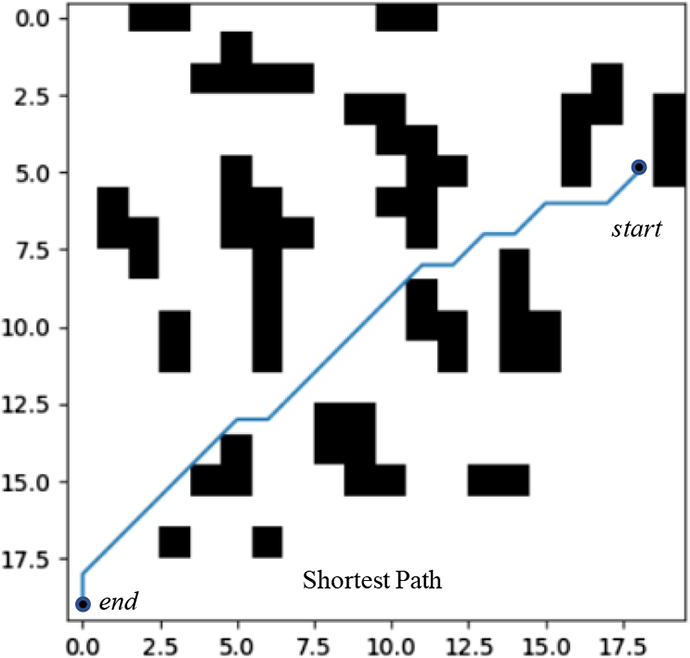
To verify the effectiveness of the proposed algorithm, this experiment compares other path planning algorithms in four different typical obstacle scenes. These scenarios are shown in Figure 7, four kinds of obstacle environments.

Figure 7.

((a) to (d)) Four obstacles with different scenes.

They separately express the location of obstacles locate near the starting point, near the terminating point, in the middle of path with simple distribution, and in the middle of path with complex distribution. Assuming that the start point is (0,0) and the end point is (19,19), the experiment runs 100 times. The planned shortest paths are shown with the straight line in Figure 7.

Here, the number of population is 40, α = 1, β = 27, ρ = 0.2 in the traditional ACO and A-APFACO algorithm, α = 1.1, β = 12, ρ = 0.5 in the ACO-PDG algorithm, crossover probability is 0.8, mutation probability is 0.2 in GA algorithm, inertia weight is 0.9, and learning factor c ₁ = 2, c ₂ = 2 in the PSO algorithm.

From Table 5, in the scene (a), all the paths are 28.042, but A* algorithm cannot converge. In the scene (b), the shortest path planned by ACO-PDG, A-APFACO, and PSO is 28.042. In the scene (c), the entire algorithm can plan the shortest path, which is 27.456. In the scene (d), the shortest path is planned by A-APFACO and genetic algorithm. Compared to other algorithms, our A-APFACO algorithm gets all the shortest path in the four scenes. As a result, A-APFACO has better performance of path planning in the four obstacle scenes.

Table 5.

The shortest path length under four obstacle scenes.

	Scene (a)	Scene (b)	Scene (c)	Scene (d)
Traditional ACO	28.042	28.870	27.456	29.213
ACO-PDG	28.042	28.042	27.456	29.213
A-APFACO	28.042	28.042	27.456	28.627
GA	28.042	29.456	27.456	28.627
PSO	28.042	28.042	27.456	29.213
A*	/	/	27.456	29.213

The convergence curves of traditional ACO, ACO-PDG, A-APFACO algorithms in complex scenes are shown in Figure 8. In scene (c), the convergence iterations of the three algorithms are 7, 11 and 8 respectively with similar performance. In the scene (d), only A-APFACO can plan a better path, and the algorithm converges only after four iterations. Experimental results show that the proposed method has better robustness for complex scene.

Figure 8.

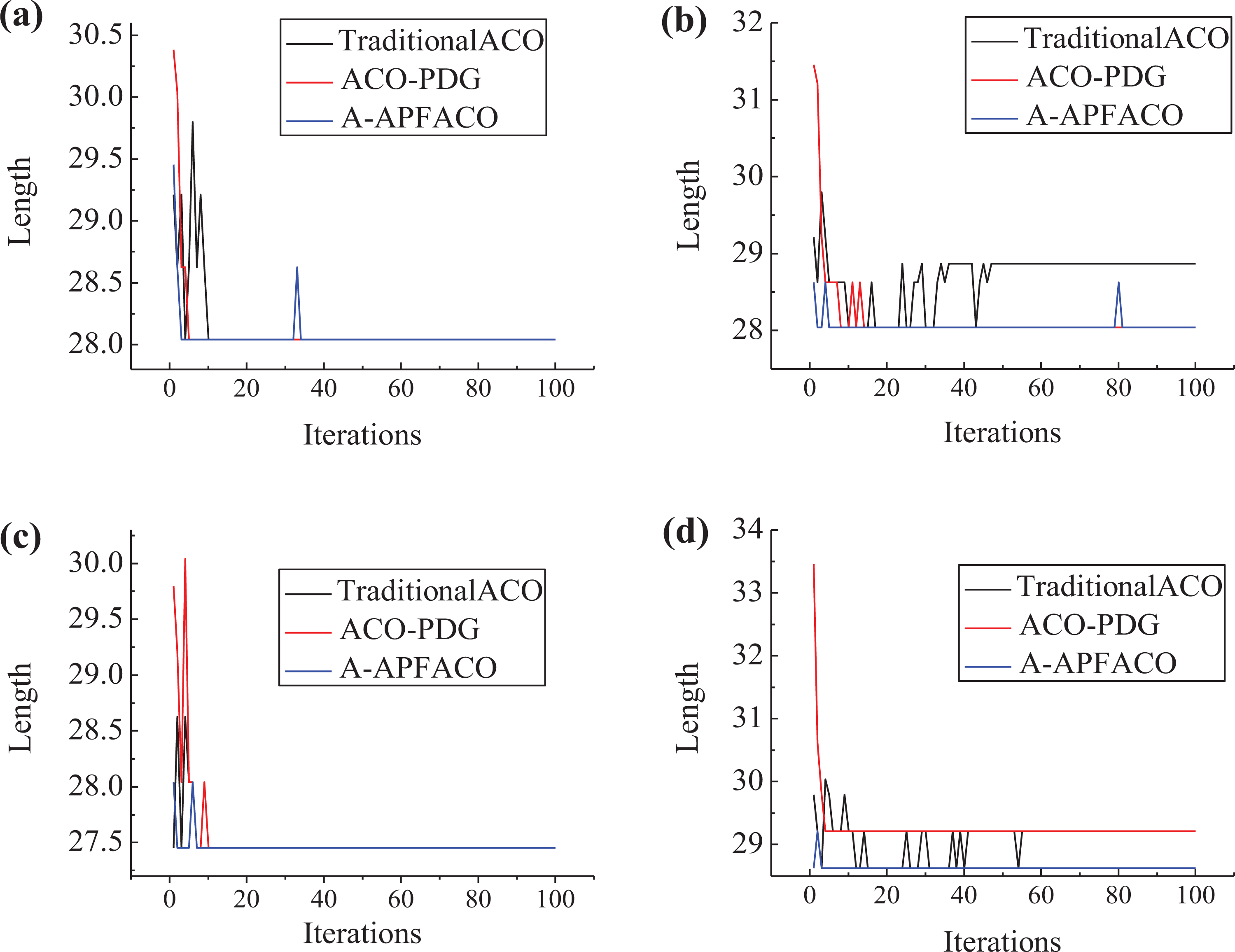
((a) to (d)) Convergence curves of three algorithms under complex scenes.

Dynamic obstacle avoidance experiment

This experiment is used to verify the effectiveness of the strategy for predictable dynamic obstacle avoidance. In the experiment, a 20 × 20 grid map was used with a moving speed of one step per second.

Experiment 3: Predictable obstacle avoidance of two targets

1. Opposite motion.

This experiment verifies the strategy of obstacle avoidance when two targets collide in opposite motion. In Figure 9, the red “*” represents R ₁, and the blue “•” is R ₂, represents the collision point.

Figure 9.

((a) and (b)) The opposite movement of two targets under obstacles.

The starting point of robot R ₁ is (19, 10) and the ending point is (1, 10). The starting point of robot R ₂ is (1, 10) and the ending point is (19, 10). The priority of R ₁ is higher than that of R ₂. The motion path planned by ant colony algorithm of R ₁ is 7 → 6 → 5 → 3 → 2, and that of R ₂ is 1 → 3 → 5 → 6 → 7. It can be seen in Figure 9, there will be a collision in opposite directions at the position of node 5, and there are obstacles beside the collision point.

Implement obstacle avoidance strategy 1, the motion path of R ₁ is 7 → 6 → 5 → 3 → 2, and that of R ₂ is 1 → 3 → 5 → 4 → 4 → 4 → 5 → 6 → 7, as shown in Figure 9(b). Here the second “4” in the path of R ₂ represents that R ₂ stopped a step at node 4. In the later experiments, if there are many identical nodes in the traveling path of robot, it means the same thing, and no further explanation is given.

2. Codirectional motion.

This experiment verifies the strategy of obstacle avoidance when two targets collide in codirectional motion. In Figures 4 to 9, the red “*” is R ₁, and the blue “•” is R ₂, is the collision point.

The starting point of robot R ₁ is (19, 10) and the ending point is (0, 10). The starting point of robot R ₂ is (13, 10) and the ending point is (0, 10). The priority of R ₁ is higher than that of R ₂. The speed of R ₁ is two steps per second and R ₂ is one step per second. The motion path planned by ant colony algorithm of R ₁ is 1 → 3 → 5 → 7 → 9, and that of R ₂ is 3 → 4 → 5 → 6 → 7 → 8 → 9. It can be seen from Figure 10 that there will be a collision in codirection at the position of node 5.

Figure 10.

((a) and (b)) The codirectional movement of two targets under obstacles.

Implement obstacle avoidance strategy 1, the motion path of R ₁ is 7 → 6 → 5 → 3 → 2, and that of R ₂ is 1 → 3 → 5 → 4 → 4 → 4 → 5 → 6 → 7, as shown in Figure 10(b).

3. Intersectional motion.

This experiment verifies the strategy of obstacle avoidance when two targets collide in intersection motion. In Figure 11, the red “*” represents R ₁, and the blue “•” is R ₂, is the collision point.

Figure 11.

((a) and (b)) The intersection movement of two targets under obstacles.

The starting point of robot R ₁ is (0, 14) and the ending point is (9, 7). The starting point of robot R ₂ is (0, 6) and the ending point is (9,15). The priority of R ₁ is higher than that of R ₂. It can be seen in Figure 11, according to the route planned by ant colony algorithm, there will be a collision at the position of node 10.

Implement obstacle avoidance strategy 3, R ₂ with low priority stops two steps at node 4 until R ₁ passes and R ₂ continues to move forward. The motion path of R ₁ is 6 → 7 → 8 → 9 → 10 → 11 → 12, and that of R ₂ is 1 → 2 → 3 → 4 → 4 → 4 → 10, as shown in Figure 11(b).

Experiment 4: Comprehensive movement of three targets

This experiment verifies the strategy of obstacle avoidance when three targets collide. In Figure 12, the green “+” represents R ₁, the blue “•” is R ₂ and the red “*” represents R ₃, represents the collision point.

Figure 12.

((a) and (b)) Comprehensive movement of three targets.

The starting points of robot R ₁, R ₂, and R ₃ are (19,0), (19,1), and (19,10), respectively, and the ending points of robot R ₁, R ₂, and R ₃ are (0,19), (6,14), and (0,10).

The motion path planned by ant colony algorithm of R ₁ is 9 → 10 → 11 → 4 → 12 → 13 → 14, and that of R ₂ is 7 → 6 → 5 → 4 → 3 → 2 → 1, R ₃ is 1 → 2 → 3 → 4 → 5 → 6 → 7. It can be seen in Figure 12, there will be a collision at the position of node 4.

As can be seen from Figure 12, at node 4, R ₁ will intersect with R ₂ and R ₃, while R ₂ and R ₃ are in opposite motion. If the priority is R ₂ > R ₃ > R ₁, R ₁ adopts the stop obstacle avoidance strategy in the safe range, while R ₃ with the second priority avoids at node 8. After robot R ₂, which has the highest priority, moves out of the safe range, R ₃ and R ₁ move in turn according to the original planning path. The process of obstacle avoidance is completed.

Implement obstacle avoidance strategy 1 and 3, the motion path of R ₁ is 9 → 10 → 11 → 11 → 11 → 11 → 11 → 11 → 11 → 11 → 4 → 12 → 13 → 14, and that of R ₂ is 7 → 6 → 5 → 4 → 8 → 8 → 8 → 4 → 3 → 2 → 1, R ₃ is 1 → 2 → 3 → 4 → 5 → 6 → 7.

Experiment 5: Dynamic avoidance of unpredictable obstacles

This experiment is designed to verify the strategy of dynamic avoidance of unpredictable obstacles. In Figures 4 to 9, the red “*” represents R ₁, and the blue “•” is R ₂, represents the collision point. Suppose the robot R ₁ cannot predict where it will collide with R ₂. And the priority of R ₂ is higher than that of R ₁.

In Figure 13, the distance and angle are calculated based on the grid in the map. Assuming the detection radius r of the robot R ₁ is 8, the safe distance h = 1.5. At t + 1 moment, when the robot R ₁ reaches point A, it detects that R ₂ reaches point C. At the next moment, R ₁ moves to point B and R ₂ moves to point D. According to formula (13), L _min ≈ 0, L _min is less than the safe distance, which means that the two robots will collide at some point. At this time, robot R ₁ stops at point B, R ₂ continues to move to point E. Here, according to formula (17), $L_{min}^{'}$ was calculated again, $L_{min}^{'} = 1.41 < h$ , so R ₁ keeps stopping at point B until R ₂ passes through. Then R ₁ moves following the original route.

Figure 13.

((a) and (b)) Dynamic prediction model.

After completing the obstacle avoidance, the motion path of R ₁ is A → B → B → B → E.

Table 6 presents the shortest distance predicted by R ₂. Because R ₁ stops avoiding at point B, the azimuth angle $θ_{1}$ between R ₂ and R ₁ is null.

Table 6.

Geometric model table.

Location of R ₂	Distance between R ₂ and R ₁ (unit)	cos θ ₁	d _min	Measure
C	4	0.785	Null	Move
D	2	0.785	2.6 × 10⁻¹⁵	Avoid
E	1.41	Null	1.41	Avoid

Comparative experiment of dynamic obstacle avoidance

In this section, the effectiveness of the proposed method is further verified by comparing the unpredictable dynamic obstacle avoidance strategy with the dynamic obstacle avoidance strategy in the literature.^18,20.

Figure 14 shows the 2D grid environment map used in the comparative experiment. The rectangular box in the figure is the area involved in the subsequent obstacle avoidance experiment.

Figure 14.

Grid map of comparative experiment.

Experiment 6: Dynamic obstacle avoidance of robot with constant velocity

As shown in Figure 14, the red “*” represents R ₁, and the blue “•” is R ₂, represents the collision point. The speed of R ₁ is one step per second, R ₂ is two steps per second, and the speed remains constant. The detection radius of R ₂ is 8, and the priority of R ₁ is higher than that of R ₂.

Figure 15(a) shows the robot’s path map formed according to our obstacle avoidance strategy. Within the detection radius of the robot, the collision will be judged according to formula (13) for each position the machine travels. When R ₁ moves to position 3 and R ₂ moves to position 11, R ₂ calculates L _min ≈ 0. And the two robots will collide at a point in front. At this time, R ₂ stops at position 11 and starts obstacle avoidance. Finally, the motion path of R ₁ is 1 → 2 → 3 → 4 → 5 → 6 → 7 → 8, the motion path of R ₂ is 9 → 10 → 11 → 11 → 11 → 12 → 5 → 13 → 14 → 15. R ₂ avoid obstacle successfully.

Figure 15.

((a) to (c)) Contrast experiment with constant speed.

Figure 15(b) is a path map of the robot formed by adopting the obstacle avoidance strategy in the study by Wang et al.¹⁸ Because the hypothesis of the strategy is that the dynamic collision point is known, the algorithm cannot calculate the collision point for the obstacles suddenly appearing in the path, and the obstacle avoidance fails. R ₁ and R ₂ collide at position 5. The motion path of R ₁ is 1 → 2 → 3 → 4 → 5, and that of R ₂ is 6 → 7 → 8 → 9 → 5.

Figure 15(c) shows the path map of the robot formed by the obstacle avoidance strategy in the study by Wang.²⁰ Since the speed of the robot remains the same, according to the obstacle avoidance algorithm, we can calculate that collision will occur, start the obstacle avoidance strategy, R ₂ accelerates the movement, and the speed will return to the original after the obstacle avoidance is successful. The motion path of R ₁ is 1 → 2 → 3 → 4 → 5 → 6 → 7 → 8, and that of R ₂ is 9 → 10 → 11 → 5 → 12 → 13.

Experiment 7: Dynamic obstacle avoidance in case of sudden change of robot speed

As shown in Figure 16, the red “*” represents robot R ₁, and the blue “•” represents robot R ₂, is the collision point. The initial velocity of R ₁ is two steps per second, R ₂ is one step per second. The detection radius of R ₂ is 8, and the priority of R ₁ is higher than that of R ₂. When R ₁ is in position 3, the speed changes suddenly for some reason, and R ₁ speed changes to one step per second.

Figure 16.

((a) to (c)) Contrast experiment with variable speed.

Figure 16(a) is the path map of the robot formed according to our obstacle avoidance strategy. Within the detection radius of robot R ₂, the collision will be judged according to formula (13) for each position the machine travels. When R ₂ is in position 8, R ₁ is in position 1 and enters R ₂ detection range. Then, R ₂ moves to position 9, R ₁ moves to position 2, and the speed suddenly changes to one step per second. Then, when R ₁ is at 4, R ₂ is at 12 and R ₂ is calculated to be L _min ≈ 0, the collision will occur at a later position. R ₂ starts obstacle avoidance strategy 3, stops two steps at position 12 and continues to move. The movement path of R ₁ was 1 → 2 → 3 → 4 → 5 → 6 → 7, and that of R ₂ was 8 → 9 → 10 → 10 → 10 → 4 → 11 → 12 → 13. R ₂ avoided obstacles successfully.

Figure 16(b) is a path map of the robot formed by adopting the obstacle avoidance strategy in the study by Wang et al.¹⁸ Because the assumption of the strategy is that the collision point is known, the algorithm cannot calculate the collision point for the obstacles that suddenly appear in the path and the speed changes. The obstacle avoidance fails, R ₁ and R ₂ collide at position 4. The motion path of R ₁ is 1 → 2 → 3 → 4, and that of R2 is 5 → 6 → 7 → 4.

Figure 16(c) is the path map of the robot formed according to the obstacle avoidance strategy in the study by Wang.²⁰ Because of the sudden change of R ₁’s speed in position 3, and the change of moving obstacle’s speed is not considered in the obstacle avoidance strategy. It is impossible to use acceleration or deceleration strategy to avoid obstacles. The obstacle avoidance fails, and R ₁ and R ₂ collide in position 4.

Conclusion

In this article, for the issue of lunar robot path planning, a heuristic function of ant colony algorithm is improved by adjusting the heuristic function dynamically. By adding adaptive parameters, the success rate of shortest path planned by ant colony algorithm is improved, while the convergence speed is reduced in complex environments. For the predictable and unpredictable dynamic collision problems in the moving route of lunar robot, the corresponding obstacle avoidance strategies are proposed. Especially for detecting unpredictable dynamic obstacles, a collision prediction model based on geometric estimation is proposed, which can avoid collision between robots. The simulation results show the effectiveness of the proposed method. The proposed method enables the lunar robot to travel in the s energy-saving path, that is, the shortest path, and effectively avoids collisions with each other.

Footnotes

Declaration of conflicting interests

The author(s) declared no potential conflicts of interest with respect to the research, authorship, and/or publication of this article.

Funding

The author(s) disclosed receipt of the following financial support for the research, authorship, and/or publication of this article: This work was supported by Shanghai Aerospace Science and Technology Innovation Fund (SAST2018-086).

ORCID iD

Shinan Zhu

References

Ammar

Bennaceur

Châari

, et al. Relaxed Dijkstra and A* with linear complexity for robot path planning problems in large-scale grid environments. Soft Comput 2016; 20(10): 4149–4171.

Hayat

Kausar

. Mobile robot path planning for circular shaped obstacles using simulated annealing. In: 2015 international conference on control, automation and robotics, Singapore, 20–22 May 2015, pp. 69–73. IEEE.

Patle

Parhi

DRK

Jagadeesh

, et al. Matrix-binary codes based genetic algorithm for path planning of mobile robot. Comput Electr Eng 2018; 67: 708–728.

Storn

Price

. Differential evolution—a simple and efficient heuristic for global optimization over continuous spaces. J Global Optim 1997; 11(4): 341–359.

Shao

Peng

, et al. Efficient path planning for UAV formation via comprehensively improved particle swarm optimization. ISA Trans 2020; 97: 415–430.

Dorigo

Maniezzo

Colorni

. Ant system: optimization by a colony of cooperating agents. IEEE Trans Syst Man Cybern B Cybern 1996; 26(1): 29.

Wang

Shi

. Comparative analysis of ant colony algorithm with simulated annealing and genetic algorithm. Wirel Interconnect Technol 2015; (13): 126–127.

Garip

Karayel

Ozkan

, et al. Path planning for multiple mobile robots using A* algorithm. Acta Physica Polonica 2017; 132(3): 685–688.

Wang

Yang

, et al. Optimization of dynamic shared bike scheduling based on ant colony. J Nanchang Inst Eng 2019; 38(3): 71–76.

10.

Stutzle

Hoos

The MAX-MIN ant system and local search for the traveling salesman problem. In: Proceedings of IEEE international conference on evolutionary computation, Indianapolis, IN, USA, 13–16 April 1997, pp. 309–314.

11.

Liu

Yang

Liu

, et al. An improved ant colony algorithm for robot path planning. Soft Comput 2017; 21(19): 5829–5839.

12.

Cheng

Miao

, et al. An improved ACO algorithm for mobile robot path planning. In: 2016 IEEE international conference on information and automation (ICIA), Ningbo, China, 1–3 August 2016, pp. 963–968. IEEE.

13.

Long

Gong

Dai

, et al. Mobile robot path planning based on ant colony algorithm with A* heuristic method. Front Neurorobotics 2019; 13: 15.

14.

Akka

Khaber

. Mobile robot path planning using an improved ant colony optimization. Int J Adv Robot Syst 2018; 15(3): 1–7.

15.

Yang

Miao

, et al. A new robot navigation algorithm based on a double-layer ant algorithm and trajectory optimization. IEEE Trans Ind Electron 2018; 66: 8557–8566.

16.

Alonso-Mora

Montijano

Nägeli

, et al. Distributed multi-robot formation control in dynamic environments. Auton Robot 2018; 43: 1079–1100.

17.

Chen

Tang

, et al. Dynamic path planning for autonomous driving on various roads with avoidance of static and moving obstacles. Mech Syst Signal Process 2018; 100: 482–500.

18.

Wang

Guan

, et al. Modeling and analysis of the obstacle-avoidance strategies for a mobile robot in a dynamic environment. Math Probl Eng 2015; 2015: Article ID 837259.

19.

Sun

Liu

Tian

, et al. Smart obstacle avoidance using a danger index for a dynamic environment. Appl Sci 2019; 9(8): 1589.

20.

Wang

. The optimization study on avoidance algorithm for UAV autonomous obstacle avoidance flight. Network New Media Technol 2019; 8(04): 36–39 + 51.

21.

Wang

Yang

Zhang

, et al. Robot path planning based on improved ant colony algorithm with potential field heuristic. Control Decision Making 2018; 33(10): 50–56.

22.

Jing-Gang

Hong-Lun

Chang

, et al. Modeling of dynamic collision avoidance zone for UAVS. Electron Opt Control 2014; 21(12): 30–35.

Path planning of lunar robot based on dynamic adaptive ant colony algorithm and obstacle avoidance

Abstract

Keywords

Introduction

Related work

An adaptive potential field ant colony algorithm

Environment modeling based on grid method

Adaptive potential field ant colony algorithm

Ant colony algorithm

Improvement of heuristic function

Adaptive artificial potential field ant colony algorithm

Robot dynamic obstacle avoidance strategy

Obstacle avoidance strategy

Predictable dynamic obstacle avoidance strategy

Unpredictable obstacle avoidance strategy

Experimental results and analysis

Experimental environment and evaluation indicators

Ant colony algorithm experiment

Experiment 1: Parameter choice

Experiment 2: Scene simulation

Dynamic obstacle avoidance experiment

Experiment 3: Predictable obstacle avoidance of two targets

Experiment 4: Comprehensive movement of three targets

Experiment 5: Dynamic avoidance of unpredictable obstacles

Comparative experiment of dynamic obstacle avoidance

Experiment 6: Dynamic obstacle avoidance of robot with constant velocity

Experiment 7: Dynamic obstacle avoidance in case of sudden change of robot speed

Conclusion

Footnotes

Declaration of conflicting interests

Funding

ORCID iD

References