Sage Journals: Discover world-class research

Abstract

Initial position estimation in global maps, which is a prerequisite for accurate localization, plays a critical role in mobile robot navigation tasks. Global positioning system signals often become unreliable in disaster sites or indoor areas, which require other localization methods to help the robot in searching and rescuing. Many visual-based approaches focus on estimating a robot’s position within prior maps acquired with cameras. In contrast to conventional methods that need a coarse estimation of initial position to precisely localize a camera in a given map, we propose a novel approach that estimates the initial position of a monocular camera within a given 3D light detection and ranging map using a convolutional neural network with no retraining is required. It enables a mobile robot to estimate a coarse position of itself in 3D maps with only a monocular camera. The key idea of our work is to use depth information as intermediate data to retrieve a camera image in immense point clouds. We employ an unsupervised learning framework to predict the depth from a single image. Then we use a pretrained convolutional neural network model to generate depth image descriptors to construct representations of the places. We retrieve the position by computing similarity scores between the current depth image and the depth images projected from the 3D maps. Experiments on the publicly available KITTI data sets have demonstrated the efficiency and feasibility of the presented algorithm.

Keywords

Initial position estimation visual localization multimodal data matching

Introductions

Localization is an essential ability for mobile robot systems such as self-driving cars. It is the prerequisite for autonomous navigation of such robots.^1,2 While global positioning system (GPS) signals can provide position estimates at a global scale, it suffers from substantial errors in urban canyons and does not provide sufficiently accurate estimates indoors.³ An effective approach to mobile robot localization is to match sensor data against a previously acquired map. Today, map providers already capture 3D light detection and ranging (LiDAR) data to build large-scale maps. LiDARs provide accurate range measurements in point cloud data type but are typically expensive and bulky. Meanwhile, monocular cameras are low-cost, lightweight, and widely available, but do not directly provide range information. Using a LiDAR for mapping and a monocular camera for localization exploits the advantages of both sensors.

However, correlational studies are not aiming for global localization, and they need a rough estimate of the initial position in the map to perform a precise localization.⁴ Initial position estimation, which is usually gained by GPS, is generally given as a prior information in tracking tasks of a full six-degree-of-freedom (6-DoF) camera pose. Initial position estimation is similar to place recognition in the field of computer vision, and it aims at locating a mobile robot in a larger scale environment.

In this article, we present a method to estimate the initial position of a camera within a given 3D LiDAR map using a convolutional neural network (CNN). It enables a mobile robot to estimate a coarse position of itself in 3D maps with only a monocular camera and no GPS assistance. The key idea of our work is to use depth information as intermediate data to retrieve a camera image in point clouds. With a satisfying result of predicting the depth information from the single camera image, it is possible to match such depth information from the camera with the depth projected from the LiDAR map by computing similarities of the two depth images.

We employ an unsupervised learning framework to predict the depth from a single image. Meanwhile, we make a set of depth images projected from the given point clouds maps, whose positions are already known. Then we use a pretrained CNN model to generate the representations of the depth images. We retrieve the position by computing similarity scores between the current depth image and the depth images projected from the 3D maps. The overview of the proposed method is shown in Figure 1. Experiments on the publicly available KITTI data sets have demonstrated the efficiency and feasibility of the presented algorithm.

Figure 1.

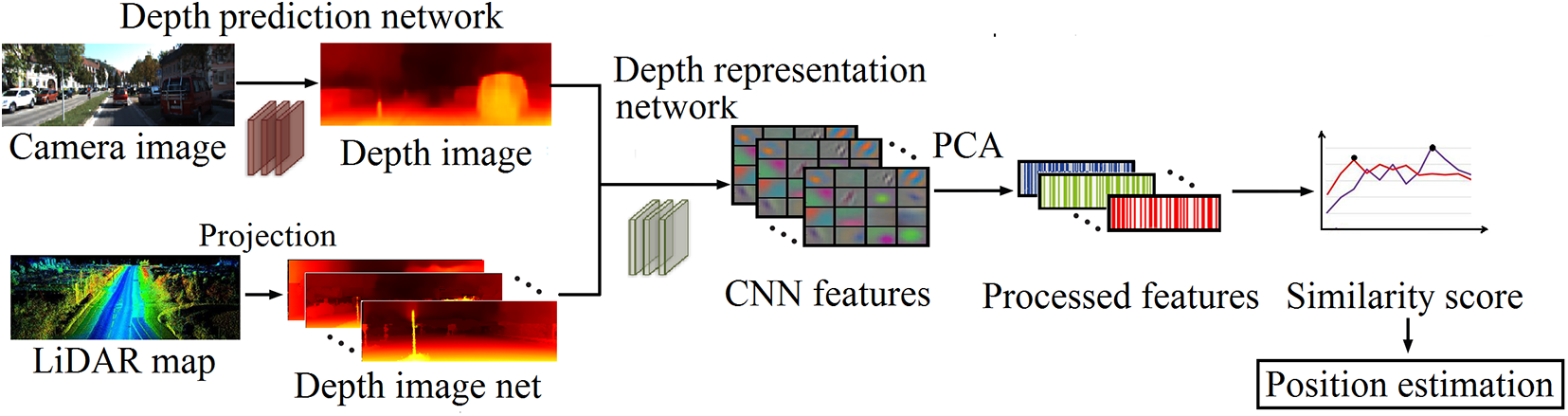
Overview of the proposed CNN-based position estimation system. The camera images are predicted to depth image through a depth prediction network and the 3D LiDAR map is projected to a set of depth images. We use a pretrained CNN model to obtain CNN feature to construct representations of the depth images. The features are then dimensionally reduced and are used to compute similarity score, based on which we estimate the positions. CNN: convolutional neural network; LiDAR: light detection and ranging.

In summary, we propose a coarse estimation of initial position of a monocular camera in 3D LiDAR maps. Our contributions can be summarized as follows:

We design a coarse initial position estimation method of a monocular camera in 3D LiDAR map with no prior localization information in a large-scale environment.

We solve the multimodal data-retrieving problem by using depth information as intermediate data. We use an unsupervised learning network to get the depth of a monocular image, and then match it to the depth map of the point cloud projection by a CNN model. Our method is versatile with no retraining of the network in different scenarios.

Related work

Visual localization has received great attention in computer vision. However, it still remains a challenging problem. It can be categorized into initial position estimation and precise localization.

Initial position estimation is similar to place recognition. Given a query image and a set of database images, the approaches retrieve the closest place in the map by leveraging different feature matching strategies. Most of the state-of-the-art place recognition algorithms take advantage of Bag-of-Visual-Words (BoVW)^5
–7 model, which is applied to image classification initially. BoVW model clusters the feature descriptors, such as scale-invariant feature transform or speeded up robust features,^8,9 using a large number of images, and produces a dictionary that contains many “words,” and a word can be considered as a representative of several similar features. When a new image comes, the feature descriptors are computed, and the image is represented based on whether the features occur in the dictionary. However, BoVW-based approaches have several drawbacks because they usually rely on traditional features. Some features are invariant toward illumination or scale but complex in computing while others may be efficiency but less distinctive, they may fail when there are significant variations in appearance between images.

Due to the enormous development of CNNs and deep learning,^10
–12 a recent trend in autonomous robots is to exploit learned features instead of traditional handcrafted features to tackle visual problems. CNN has been used to achieve excellent performance on a variety of tasks, such as image classification¹³ and image retrieval.¹⁴ Since place recognition is substantially similar to image classification and image retrieval (the critical step of these problems are all obtaining good representations for images), it is reasonable to expect that CNN features can be used to detect loops for visual short for simultaneous localization and mapping (SLAM) systems. Chen et al.¹⁵ presented a method using features learned by CNN models with spatial and sequential filter. The method outperformed most traditional handcrafted features-based techniques. Arandjelovic et al.¹⁶ designed a new CNN architecture to tackle large-scale place recognition problem. The model was trained in an end-to-end manner, and results showed that their representations significantly outperformed off-the-shelf CNN features on two particular data sets. All these methods are proposed to solve the initial position estimation problem based on camera images, not focusing on large-scale initial position estimation based on heterogeneous data.

For precise localization of a robot, it need a coarse estimation of initial position. With range scanning devices becoming standard equipment in mobile robotics, a large number of research have been done on exploiting the 3D LiDAR data in robotic tasks including localization, mapping, and object detection.¹⁷ Feng et al.¹⁸ proposed a 2D-3D data match method, 2D3D-MatchNet, which is an end-to-end deep network architecture to jointly learn the descriptors for 2D and 3D keypoint from image and point cloud. It is able to directly match and establish 2D-3D correspondences from the query image and 3D point cloud reference map for visual pose estimation and other recognition applications.

Some studies focus on precisely localizing a camera in LiDAR maps, which concentrate on solving the differences between camera data and LiDAR data.^19,20 Stewart and Newman²¹ used minimized normalized information distance for matching the camera and LiDAR intensities. Wolcott and Eustice²² used LiDAR reflectance images, and matched them to a camera intensity image to seek the maximum normalized mutual information. Naseer and Burgard²³ proposed a metric monocular localization using CNNs in an end-to-end fashion. It was focusing on localization of a camera in a local place like hospital and church, and was not suitable for city scale pose regression. Another work of tracking 6-DoF camera pose, CMRNet²⁴, need an initial estimate from a global navigation satellite system device. For precisely tracking, it compared RGB images and a synthesized depth image projected from a LiDAR map. Our previous work²⁵ tracked a 6-DoF pose of a monocular camera within a LiDAR map by matching sparse camera point clouds acquired from direct sparse odometry (DSO-SLAM) with an a priori LiDAR map to find corresponding points. This work is also in need of a coarse estimation of initial position as a prior information.

Although these methods had satisfying results in localization problem among multimodal sensor data, they were merely suitable for local localization with a coarse estimation of initial position needed. The robot has to recognize the initial position before performing a precise localization. In this article, we use a CNN model to estimate the coarse initial position of a robot in a large-scale environment. We process the 3D point cloud map into a set of depth images with position tag and try to retrieve a monocular camera image in it.

Proposed method

In this section, we present in detail our method to construct, train, and utilize a novel CNN for estimating the initial rough position of a monocular camera within a large-scale 3D LiDAR map. The given map can cover entire neighborhoods or even entire city, with numerical range reaching tens of kilometers.

We employ an unsupervised learning framework to predict the depth from a single camera image. On the other hand, we project the 3D LiDAR map into a set of depth images with ground-truth position. Then we use a pretrained CNN model to generate depth image descriptors to construct representations of the places, which are high-dimensional vectors. After that, we define similarity score based on the processed vectors and retrieve the position by computing similarity score between current depth image and the depth map set.

Single image depth prediction

There are some recent significant works on unsupervised training of single image depth prediction.²⁶ Zhou et al.²⁷ introduce joint unsupervised learning of ego-motion and depth from multiple unlabeled frames. It performs comparably with supervised methods that use either ground-truth pose or depth for training. Ranjan et al.²⁸ exploit consistency between depth and optical flow to improve performance. Inspired by the framework in the literature,²⁷ we use an end-to-end learning pipeline that utilizes the task of view synthesis for the supervision of single-view depth. Our method uses single-view depth and multi-view pose constraints, with a loss based on warping nearby views to the target using the computed depth and pose. The framework is shown in Figure 2.

Figure 2.

Depth prediction framework. The depth network takes in view image at time $t, t - 1, t + 1$ and outputs a per-pixel depth map $D_{t}, D_{t - 1}, D_{t + 1}$ . The pose network outputs the relative camera poses ( $T_{t \to t - 1}, T_{t \to t + 1}$ ). The projection ${D^{'}}_{t} (p)$ can be calculated by $D_{t - 1} (p), D_{t + 1} (p)$ and the poses using bilinear interpolation.

We adopt the DispNet²⁹ as depth network with multi-scale side predictions. The structure of the network is shown in Figure 3, it is a typical encoder-decoder architecture. The width and height of each rectangular block indicate the output channels and the spatial dimension of the feature map at the corresponding layer, respectively. The kernel size is 3 for all the layers except for the first four conv layers with 7, 7, 5, 5, respectively, and the number of output channels for the first conv layer is 32.

Figure 3.

Structure of the depth prediction network. We use encoder-decoder architecture. The width and height of each rectangular block indicate the output channels and the spatial dimension of the feature map at the corresponding layer, respectively.

All conv layers are followed by rectified linear unit (ReLU) activation except for the last two layers, where we use $α = 10$ and $β = 0.1$ in the activation function

f (x) = \frac{1}{α * sigmoid (x) + β}

This constrains the predicted depth to be always positive within a reasonable range.

As for pose constraints, it estimates the relative poses between the current view and each of the other view based on optical flow constraints. The projection loss is defined as the loss function to train the CNN. For training image sequence $< I_{1}, \dots, I_{N} >$ , the loss function is

L = \sum_{N} \sum_{p} | {D^{'}}_{t} (p) - D_{t} (p) |

The framework can be trained simply using sequences of images with no manual labeling ground-truth depth.

Depth images from point cloud projections

Now we have the depth information of the camera image. To correlate the depth of the camera with the 3D point cloud map, we divide and project the 3D point cloud map into a set of depth images.

The 3D point cloud map was divided along the road into a collection of small complementary point cloud areas. Since the scenario of our study is position estimation of unmanned vehicles and other ground robots, we project the divided point cloud map into a virtual image plane, positioned at the initial guess of the camera pose that perpendicular to the robot’s motion. That is, if the robot moves along the X axis, the 3D point cloud needs to be projected onto the plane formed by the Y–Z axis.

We use Point Cloud Library to project the points onto a plane model. The parametric model is given through a set of coefficients. For plane model, the coefficients equation should be

a x + b y + c z + d = 0

In the urban environment, the map would be projected vertically to the road. In that case, the 3D map can be preprocessed offline to reduce the time of online calculation and improve the processing speed. Otherwise, in a roadless environment, map projection needs to know the robot’s motion direction and project the map onto a plane perpendicular to the robot’s motion direction. The motion can be learned by optical flow constrains in sequential images as described in single depth prediction. We define the depth sets projected from the 3D point cloud map as

\hat{D} = {{\hat{D}}_{i} | {\hat{D}}_{i} \in ℝ^{2}, i = 1, \dots, D}

Since the given map initially has accurate location information, each of the processed depth images is marked with a corresponding position label for subsequent estimation.

CNN-based depth feature representation

To match the depth information of the camera image and the point cloud, we propose a pretrained CNN to calculate the whole depth image-level representations. We use a publicly available pretrained CNN called OverFeat,³⁰ which has been released as a feature extractor to provide powerful features for computer vision research. Figure 4 illustrates the architecture of the network, which consists of convolutional, max-pooling, and fully connected layers. For different convolutional layers, each contain 96–1024 kernels of size $3 \times 3$ to $7 \times 7$ . ReLU³¹ is used as a nonlinear activation function and max-pooling layers are used to build robustness to intra-class deformations with $3 \times 3$ to $5 \times 5$ kernels. We detail the architecture sizes in Table 1. Each image is divided to $256 \times 256$ pixels so that the smallest dimension is 256 pixels. We then extract five random crops (and their horizontal flips) of size $221 \times 221$ pixels and present these to the network.

Figure 4.

Architecture for depth representation network. The network takes images of size $221 \times 221$ as input, and the output is a 4096-element vector corresponding to score. We use the output as depth image representation.

Table 1.

Architecture specifics for the depth description network.

Layer	1	2	3	4	5	6	7	8
Stage	Conv + max	Conv + max	Conv	Conv	Conv	Conv + max	Full	Full
Channels	96	256	512	512	1024	1024	4096	4096
Filter size	$7 \times 7$	$7 \times 7$	$3 \times 3$	$3 \times 3$	$3 \times 3$	$3 \times 3$	—	—
Conv stride	2	1	1	1	1	1	—	—
Pooling size	$3 \times 3$	$2 \times 2$	—	—	—	$3 \times 3$	—	—
Pooling stride	3	2	—	—	—	3	—	—

Conv: convolution; max: max-pooling operation; full: fully connected layer.

To improve the power of representing images, we perform principal components analysis (PCA)³² to the output vector. In PCA, we find the directions in the data with the most variation, that is, the eigenvectors corresponding to the largest eigenvalues of the covariance matrix, and project the data onto these directions. By doing so, we project those high-dimension features into a lower-dimensional space, which makes the detecting process more efficient and more accurate. In this work, we reduce the dimensionality of feature from 4096 to 500.

Similarity score

The crucial part of the position estimation problem is the estimation of the similarity between the depth images. For this purpose, we calculate the distance between CNN feature vectors of different depth images and define the similarity score for pairwise images. We use the Euclidean distance of vectors to measure the similarity between depth images.

For the final CNN feature vectors $V^{D_{i}} \in ℝ^{500}$ of input depth image D_i , we normalize the vectors and calculate the Euclidean distance as follows

d (i, j) = | | \frac{V^{D_{i}}}{∥ V^{D_{i}} ∥_{2}} - \frac{V^{D_{j}}}{∥ V^{D_{j}} ∥_{2}} ∥_{2}

where $d (i, j)$ is the distance between image D_i and D_j , and $∥ ∥_{2}$ is the $ℓ_{2}$ -norm of the vector. Hence, if depth image D_i and D_j have a higher similarity, the $d (i, j)$ will be smaller. Then we define the similarity score between depth images as

S (i, j) = 1 - \frac{d (i, j)}{max d (i, j)}

Larger values indicate higher similarity scores, and they are more likely to be the same position for the corresponding depth images and vice versa. By calculating the similarity score of the current camera depth D_i and the depth images in the map set $\hat{D}$ , we can obtain the highest similarity score which we regard as the same position. A normalized distance is used in our case to obtain the score values lies in [0, 1] for measurement purpose.

Experiments and evaluation

In this section, we describe the details of the conducted experiments and evaluate their results. We evaluated our method on the publicly available KITTI data set.³³ The KITTI odometry data set provides sequences of images from a monocular camera, Velodyne HDL-64E LiDAR scans, and the ground-truth poses. Extrinsic calibration between the camera and the LiDAR as well as intrinsic calibration for the monocular camera are also provided.

We selected images from KITTI sequence 00–07, including crowded block, broad street, highway, and landscaping scenarios. We first test the single image depth prediction result and point cloud map projection result. Then we test the validity of the proposed similarity score. At last, we compare the proposed CNN-based position estimation method against the original OverFeat³⁰ network using a precision–recall curve metric.

Single image depth prediction

We train our image depth prediction framework on KITTI image data set captured by color camera 02. The original camera image size is $1242 \times 375$ pixels, and we resized it to $416 \times 128$ pixels during training, but the depth network can be run fully convolutional for images of arbitrary size at test time. We fix the length of image sequences to be three frames and treat the central frame as the current view and the $\pm 1$ frames as the nearby views. In the training stage, we use three frames in images sequence to train the network, and use the pose constraints of the optical information in the images to optimize the depth network. In the test stage, the network can generate depth image for single image.

We implemented the system using the publicly available TensorFlow³⁴ framework.

Figure 5 shows the prediction result of a single camera image.

Figure 5.

The result of single image depth prediction. The comparison of single image depth prediction between the ground-truth depth supervision and our result. The sparse part of sky area in the ground-truth depth map is removed for visualization purpose.

We can see that although trained in an unsupervised manner, the results fit to the ground truth well, and can preserve the depth boundaries and thin structures such as trees and streetlights.

To evaluate the versatility of our depth prediction model, we directly apply our model trained on KITTI to the images of real scenes that were unseen during training (see Figure 6). Our predictions are able to capture the global scene layout reasonably well without any training on the new images.

Figure 6.

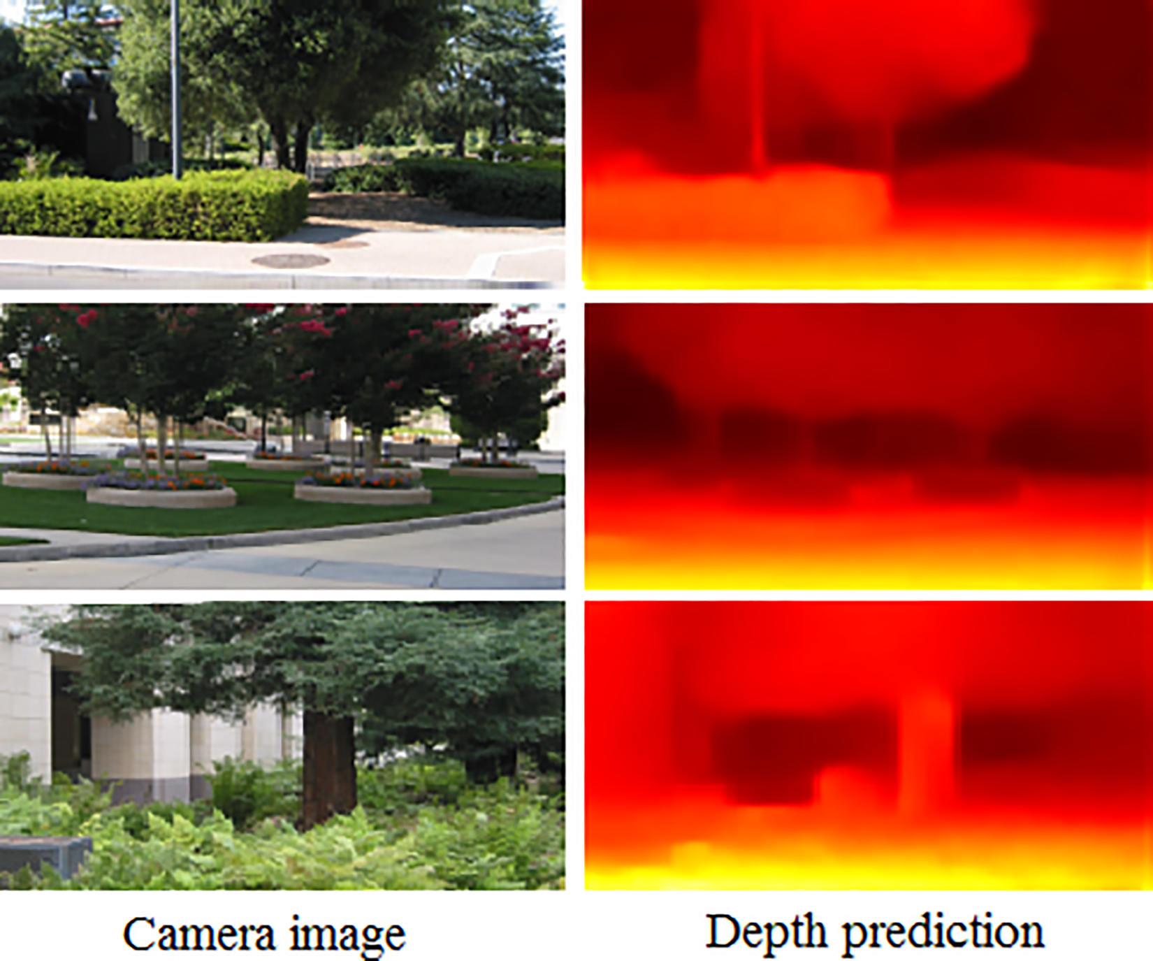
Our depth predictions on real scenes. The framework is trained on KITTI, and directly tested on real scenes.

Point cloud map projection

We perform the point cloud map projection at the segmentation distance of 20 m. We found that this threshold is better in retaining the depth characteristics without excessive segmentation.

Figure 7 shows the result of the point cloud map projection. The robot moves along the X axis, and the point clouds project onto the plane formed by the Y–Z axis. Since the data set does not have a similar point cloud projection work, there is no corresponding ground truth.

Figure 7.

The result of point cloud map projection. Three different scenes have different depth appearances.

We select three different road sections as examples, including normal road, broad space, and narrow street. After the projection, the depth images with different features are generated. We can see different features of road sections from the comparison. Different sections would have different CNN descriptors to distinguish their locations.

One hundred map segments are divided from eight sequences, KITTI 00–07, generating a candidate set of depth maps with the number of 100. This step greatly reduces the amount of map data, making it possible to quickly locate a camera in large-scale maps.

Since the map is projected based on the motion direction of the robot, we only deal with the straight road sections. The turnings have been neglected due to the change of motion direction. If the robot does not get a good matching result at the corner, it can keep matching along the movement until a better result on straight road. This operation can greatly reduce the amount of map data, making it possible to quickly locate in large-scale maps. Since our goal is to determine the coarse position of the robot in the large map, we believe that such a trade-off is reasonable.

Position estimation accuracy

We use camera images in KITTI sequence 00 as test images. The depth images produced by the above steps are the size of $832 \times 256$ pixels. We divided each depth image into three images of $256 \times 256$ pixels to fit the network and take the average of the three output vectors as the representation of it.

According to the steps described in the similarity score, we calculate the similarity score for the input depth image using processed CNN features and find the best match with the highest score.

Figure 8 shows the similarity score results of three example images D_A , D_B , D_C within the map candidates’ sequence. The candidate that has the highest score is considered the corresponding place. For the result that the score difference is less than a threshold, camera images should be included for further calculation. If continuous camera images correspond to the same result at a higher average score, or the results are continuous, the result is considered more likely the right position. All camera images in the data set have the corresponding score curve like these three examples, and we can find the best result with the highest score.

Figure 8.

Similarity score results of depth images D_A , D_B , and D_C . Each candidate has different similarity score. The candidate that has the highest score is most similar to the input sample. Thus the corresponding position of selected candidate is the rough position of the input image.

Figure 9 shows the estimation result according to the similarity score. It shows the input sample image, the depth image generated by the sample image, and the map projection corresponding to the highest score after the calculation.

Figure 9.

The estimation result according to the similarity score. I_A , I_B , and I_C are the original image of camera view. D_A , D_B , and D_C are the corresponding depth image predicted by the depth network. ${\hat{D}}_{J}$ , ${\hat{D}}_{K}$ , and ${\hat{D}}_{Q}$ are the depth projection that has the highest corresponding similarity score.

In terms of the accuracy of the position estimation method, the method solves a multi-classification problem of finding a best solution in multiple candidates. Since the most common evaluation methods in image classification are aimed at binary classification problem, we test the method by pairing a camera image and a random chosen map depth image to see if they match. There are only two cases: yes or no. In that way, the original multi-classification problem is converted into a binary classification problem and can be evaluated by general methods.

The performance of binary classification problem is typically evaluated according to precision, recall metrics, and precision–recall curve. The matches consistent with the ground truth are true positives (TP), the matches inconsistent with the ground truth are false positives (FP), and the matches erroneously discarded by the position estimation algorithm are false negative (FN) matches. Precision is the proportion of matches recognized by the place recognition algorithm as TP matches, and recall is the proportion of TP matches to the total number of actual matches in the ground truth, that is

Precision = \frac{TP}{TP + FP}, Recall= \frac{TP}{TP+FN}

A perfect system would be one that achieves a precision of 100% and recall of 100%. By observing both of these values, we utilize the precision–recall curve, a standard method to evaluate binary classification, to quantify effectiveness of our proposed method.

Figures 10 shows the recall rate and precision rate of the method on the whole test images. The precision indicates the accuracy of the position estimation method. If the performance is better, the precision rate will remain at a high level while the recall rate increases, while a poor performance may sacrifice precision rate to improve the recall rate. From the definition of precision and recall, we can see that if the precision and recall are higher, the algorithm will be more effective, and the precision–recall curve will be closer to the upper right. As we can see from the figure, our approach achieves a higher precision and outperforms the original OverFeat method without PCA procedure.

Figure 10.

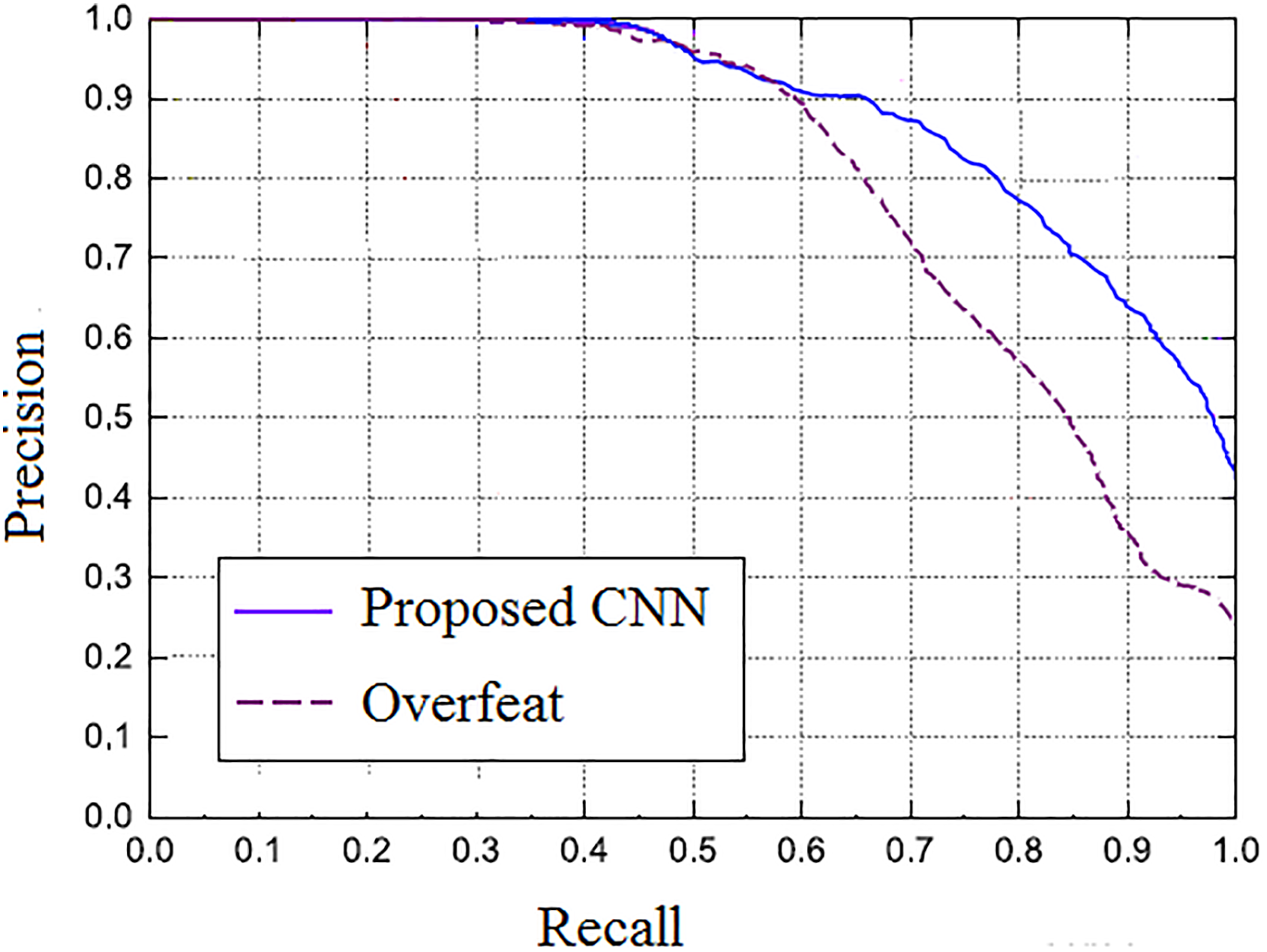
Comparison of precision–recall curves between our method and the original OverFeat network on KITTI data sets.

Conclusion

In this article, we propose a coarse initial position estimation method of a monocular camera in 3D LiDAR map with no prior localization information in a large-scale environment. Built upon unsupervised CNN framework, our method solves the multimodal data-retrieving problem by estimating depth image of a monocular image and match the depth image to the depth map projected from the point cloud, to locate the monocular image in the point cloud. Experiments on open data sets KITTI sequences have demonstrated the feasibility of the presented algorithm. Our approach achieves a high accuracy in initial position estimation. The approach uses an unsupervised framework for depth prediction, which has shown satisfying results in different scenes, and a pretrained CNN model for depth image description. Thus the model is robust and versatile with no retraining of the network in different scenarios. Further improvement toward improvement to efficiency and invariance to dynamic object changes should be considered.

Footnotes

Declaration of conflicting interests

The author(s) declared no potential conflicts of interest with respect to the research, authorship, and/or publication of this article.

Funding

The author(s) disclosed receipt of the following financial support for the research, authorship, and/or publication of this article: This work was partially supported by the National Natural Science Foundation of China (nos 61803375 and 91648204), the National Key Research and Development Program of China (nos 2017YFB1001900 and 2017YFB1301104), and the National Science and Technology Major Project.

ORCID iD

Manhui Sun

References

Yang

Scherer

, et al. Multi-camera visual SLAM for autonomous navigation of micro aerial vehicles. Robot Auton Syst 2017; 93: 116–134.

Zhang

Liu

Yin

, et al. Intelligent collaborative localization among air-ground robots for industrial environment perception. IEEE Trans Ind Electron 2019; 66(12): 9673–9681.

Liu

Zhang

Chen

, et al. Towards SLAM-based outdoor localization using poor GPS and 2.5D building models. In: 2019 IEEE international symposium on mixed and augmented reality (ISMAR), Beijing, China, 14–18 October 2019, pp. 14–18. IEEE.

Zhang

Chen

, et al. Distributed and collaborative monocular simultaneous localization and mapping for multi-robot systems in large-scale environments. Int J Adv Robot Syst 2018; 15(3): 1729881418780178.

Galvez-Lopez

Tardos

. Bags of binary words for fast place recognition in image sequences. IEEE Trans Robot 2012; 28(5):1188–1197.

Filliat

. A visual bag of words method for interactive qualitative localization and mapping. In: IEEE international conference robotics and automation, Roma, Italy, 10–14 April 2007, pp. 3921–3926. IEEE.

Yang

Jiang

Hauptmann

A G

, et al. Evaluating bag-of-visual-words representations in scene classification. In: Proceedings of the international workshop on multimedia information retrieval, Augsburg, Bavaria, Germany, 24–29 September 2007, pp. 197–206. ACM.

Sukthankar

. PCA-SIFT: A more distinctive representation for local image descriptors. In: IEEE conference on computer vision and pattern recognition, Washington, DC, USA, 27 June–2 July 2004, pp. 506–513. IEEE.

Bay

Ess

Tuytelaars

, et al. Speeded-up robust features (SURF). Comput Vis Image Und 2008; 110(3): 346–359.

10.

LeCun

Bengio

Hinton

. Deep learning. Nature 2015; 521(7553): 436–444.

11.

Bengio

Courville

Vincent

. Representation learning: a review and new perspectives. IEEE Trans Pattern Anal Mach Intell 2013; 35(8):1798–1828.

12.

Rastegari

Ordonez

Redmon

, et al. XNOR-Net: ImageNet classification using binary convolutional neural networks. In: European conference on computer vision, Amsterdam, The Netherlands, 8–16 October 2016, pp. 525–542. Cham: Springer.

13.

Krizhevsky

Sutskever

Hinton

. ImageNet classification with deep convolutional neural networks. In: Advances in neural information processing systems. Curran Associates Inc, 2012, pp. 1097–1105.

14.

Babenko

Slesarev

Chigorin

, et al. Neural codes for image retrieval. In: European conference on computer vision, Zurich, Switzerland, 6–12 September 2014, pp. 584–599.Springer International Publishing.

15.

Chen

Lowry

Jacobson

, et al. Distance metric learning for feature-agnostic place recognition. In: IEEE/RSJ international conference on intelligent robots and systems (IROS), Hamburg, Germany, 28 September–2 October 2015, pp. 2556–2563. IEEE.

16.

Arandjelovic

Gronat

Torii

, et al. NetVLAD: CNN architecture for weakly supervised place recognition. IEEE Trans Pattern Anal Mach Intell 2018; 40: 1437–1451.

17.

Levinson

Thrun

. Robust vehicle localization in urban environments using probabilistic maps. In: IEEE international conference on robotics and automation, Anchorage, AK, USA, 3–7 May 2010, pp. 4372–4378. IEEE.

18.

Feng

Ang

, et al. 2D3D-MatchNet: learning to match keypoints across 2D image and 3D point cloud. preprint 2019. arXiv: 1904.09742.

19.

Caselitz

Steder

Ruhnke

, et al. Monocular camera localization in 3D LiDAR maps. In: IEEE/RSJ international conference on intelligent robots and systems (IROS), Daejeon, South Korea, 9–14 October 2016, pp. 1926–1931. IEEE.

20.

Jaramillo

Dryanovski

Valenti

, et al. 6-DoF pose localization in 3D point-cloud dense maps using a monocular camera. In: IEEE international conference on robotics and biomimetics (ROBIO), Shenzhen, China, 12–14 December 2013, pp. 1747–1752. IEEE.

21.

Stewart

Newman

. LAPS-localisation using appearance of prior structure: 6-DoF monocular camera localisation using prior point clouds. In: IEEE international conference on robotics and automation, Saint Paul, MN, USA, 14–18 May 2012, pp. 2625–2632. IEEE.

22.

Wolcott

Eustice

. Visual localization within LIDAR maps for automated urban driving. In: IEEE/RSJ international conference on intelligent robots and systems (IROS), Chicago, IL, USA, 14–18 September 2014, pp. 176–183. IEEE.

23.

Naseer

Burgard

. Deep regression for monocular camera-based 6-dof global localization in outdoor environments. In: IEEE/RSJ international conference on intelligent robots and systems (IROS), Vancouver, BC, Canada, 24–28 September, 2017, pp. 1525–1530. IEEE.

24.

Cattaneo

Vaghi

Ballardini

, et al. CMRNet: Camera to LiDAR-Map Registration. preprint 2019. arXiv: 1906.10109.

25.

Sun

Yang

Liu

. Scale-aware camera localization in 3D LiDAR maps with a monocular visual odometry. Comput Animat Virt W 2019; 30(3–4): 1879.

26.

Eigen

Puhrsch

Fergus

. Depth map prediction from a single image using a multi-scale deep network. Adv Neur Inform Proc Syst 2014; 3: 2366–2374.

27.

Zhou

Brown

Snavely

, et al. Unsupervised learning of depth and ego-motion from video. In: Proceedings of the IEEE conference on computer vision and pattern recognition, Honolulu, HI, USA, 21–26 July 2017, pp. 1851–1858. IEEE.

28.

Ranjan

Jampani

Balles

, et al. Competitive collaboration: joint unsupervised learning of depth, camera motion, optical flow and motion segmentation. In: Proceedings of the IEEE conference on computer vision and pattern recognition, Long Beach, CA, USA, 16–20 June, 2019, pp. 12240–12249. IEEE.

29.

Mayer

Ilg

Hausser

, et al. A large dataset to train convolutional networks for disparity, optical flow, and scene flow estimation. In: Proceedings of the IEEE conference on computer vision and pattern recognition, Las Vegas, NV, USA, 27–30 June, 2016, pp. 4040–4048. IEEE.

30.

Sermanet

Eigen

Zhang

, et al. Overfeat: integrated recognition, localization and detection using convolutional networks. preprint 2013. arXiv: 1312.6229.

31.

Hara

Saito

Shouno

. Analysis of function of rectified linear unit used in deep learning. In: International joint conference on neural networks (IJCNN), Killarney, Ireland, 12–17 July 2015, pp. 1–8. IEEE.

32.

Geladi

Kowalski

. Partial least-squares regression: a tutorial. Anal chim acta 1986; 185: 1–17.

33.

Geiger

Lenz

Urtasun

. Are we ready for autonomous driving? The KITTI vision benchmark suite. In: IEEE conference on computer vision and pattern recognition, Providence, RI, USA, 16–21 June 2012, pp 3354–3361. IEEE.

34.

Abadi

Agarwal

Barham

, et al. Tensorflow: large-scale machine learning on heterogeneous distributed systems. preprint 2016 . arXiv: 1603.04467.

Convolutional neural network-based coarse initial position estimation of a monocular camera in large-scale 3D light detection and ranging maps

Abstract

Keywords

Introductions

Related work

Proposed method

Single image depth prediction

Depth images from point cloud projections

CNN-based depth feature representation

Similarity score

Experiments and evaluation

Single image depth prediction

Point cloud map projection

Position estimation accuracy

Conclusion

Footnotes

Declaration of conflicting interests

Funding

ORCID iD

References