Sage Journals: Discover world-class research

Abstract

In this study, we propose an improved iterated greedy algorithm for solving the distributed permutation flowshop problem, where there is a single robot in each factory and the makespan needs to be minimized. In the problem considered, the robot is used to transfer each job from the predecessor machine to the successor machine. A blocking constraint between machines is considered, thus jobs should remain on the completed machine while waiting for the robot. The loading and unloading times are considered and different for all of the jobs conducted by the robot, and the deteriorating time is also considered. In the proposed algorithm, first, four types of neighborhood structures are developed. Then, the simulated annealing algorithm is embedded in the proposed algorithm to enhance the exploration abilities. Furthermore, a problem-specific destruction and construction strategies are investigated. Finally, several realistic instances were generated to test the proposed algorithm, and its competitive performance was verified based on detailed experimental comparisons.

Keywords

Distributed flowshop problem deteriorating processing time iterated greedy algorithm robotic transportation

Introduction

During recent years, the intelligent manufacturing has gradually penetrated into both the industrial and academic fields.^1

–4 It is a common understanding that the intelligent manufacturing is a new production model which integrates lots of new technical means, such as intelligence production, intelligent scheduling, and integration. In the realistic production, the scheduling is generally one of the key issues in the intelligent manufacturing. The distributed permutation flowshop scheduling problem (DPFSP), as an extension of the classical flowshop scheduling problem (FSP), has gained more and more research focuses during recent years.

The definition and several types of mathematical models for the DPFSP were first proposed by Naderi and Ruiz.⁵ The DPFSP involves two main important tasks comprising assigning jobs to suitable factories and scheduling the jobs in the assigned factories.^6
–8 In the DPFSP, in addition to the number of job and factory, the factory includes a number of machines, while the machine number and other factors must also be considered.^9,10 The sequence of jobs assigned to factory f was given, where each job on each machine has a processing time.¹¹ The general objective is to minimize the total processing time.^12,13

The method to solve related DPFSP has attracted much attention. Generally, the artificial bee colony (ABC) algorithm^14

–17 and shuffled frog-leaping algorithm¹⁸ were used to solve the job shop scheduling. However, Li et al.¹⁹ used hybrid ABC algorithm to solve the problem of parallel batch distributed flowshop with deteriorating jobs. Many algorithms have been proposed for solving the DPFSP, such as tabu search (TS) algorithm,²⁰ genetic algorithm (GA),²¹ simulated annealing (SA) algorithm,²² and iterated greedy (IG) algorithm^23

–28 solved a casting scheduling problem by a new coevolutionary artificial bee colony that proposed by Pan (P-ABC). Li et al.²⁹ used a multi-objective algorithm to solve the problem of batch mixed flowshop with variable sub-batches. Deng and Wang³⁰ presented a competitive memetic algorithm to solve the multi-objective DPFSP as well as developed several local search operators in proposed algorithm. However, few studies have considered that robotic distributed flowshop problem.

At present, artificial intelligence (AI) applications are infiltrating into various industries, especially the robot that can transport jobs. In some industries, such as logistics warehouses, steel ball factories, and automobile parts factories, robots transport jobs between machines for reducing costs and worker requirements and then greatly improve the throughput in factories. He et al.³¹ and Dong et al.³² studied on the dynamics of robot system and the accuracy of robot control system. In robot scheduling and path planning, real-world flowshop systems often involve uncertainty; however, various types of metaheuristics have been developed for solving realistic optimization problems. Hurink and Knust³³ considered that jobs must be transported between machines by a single robot in the flowshop factory. Subsequently, they applied the TS algorithm to minimum manufacturing time.³⁴ Arviv et al.³⁵ developed a collaborative reinforcement learning method to solve the problem of two robots transporting jobs between successive machines on a parallel trajectory, where the objective was to obtain a robot scheduling table that minimizes the manufacturing cycle time on the machines. Che and Chu³⁶ and Che et al.³⁷ presented a multiple degrees of freedom cyclic scheduling algorithm for two robots in a no-wait flowshop with the objective of minimizing the cycle time. Che et al.³⁸ proposed an efficient bicriteria algorithm to consider a robot transportation time with an allowed small disturbance. Gultekin et al.³⁹ also considered the objectivity of minimizing cyclic time of robots and maximizing the throughput and developed a hybrid metaheuristic algorithm that combined GA with TS algorithm. Kats and Levner⁴⁰ discussed the robot path with the minimum cycle time for two-loop scheduling. Nouri et al.^41,42 proposed two NP-hard problems, that is, the flexible job shop scheduling and robot path, and they used hybrid metaheuristics to solve these problems simultaneously. Zabihzadeh and Rezaeian⁴³ considered the limitation caused by blocking in a mixed flowshop with robot, where their main contribution was to use two metaheuristic algorithms. Both Elmi and Topaloglu take into account the loading and unloading time of robots.^44,45 Chen et al.^46,47 designed two algorithms to systematically schedule the multi-robot to obtain resources and objective to improve the cost efficiency.

These literatures provide a good idea to solve the robot scheduling problem, but do not provide a good solution for the practical problems of distributed factory scheduling in the intelligent manufacturing. According to our knowledge, there is few literature aimed at solving the robot scheduling problem in DPFSP and none have applied the improved iterated greedy (IIG) algorithm to solve this problem: (1) most of the literatures about the intelligent scheduling problems consider the production in one factory; however, the distributed manufacturing features in the realistic manufacturing should be considered; (2) in the realistic production, considering the weight of jobs, the transportation process of a robot or crane should be investigated, which has less been studied; and (3) most of the studies considered to minimize the time-related objectives, such as makespan and earliness/tardiness values. However, the energy consumptions during the processing and robotic transportations should be considered simultaneously. Therefore, the IIG algorithm is proposed to solve the NP-hard problem, that is, the single-robot scheduling of distributed flowshop in this study. In the study, we add a single robot to the traditional DPFSP to transform it into an NP-hard problem and consider deteriorating time of jobs.^48
–50 The blocking constraint between machines is also considered, and jobs should remain on the completed machine while waiting for the robot. Finally, the IIG algorithm is compared with the cooperative ABC (CABC) algorithm,⁵¹ P-ABC algorithm, and TS algorithm.

The remainder of this article is organized as follows. Firstly, the constraints, mathematical models, and problem description are briefly described. Next, the canonical IG algorithms and the elaborated proposed algorithms with strategies in detail are introduced. Then, the results obtained in experiments and parameter analysis are illustrated. Finally, the study conclusions are given.

Problem formulation

Problem description

The robotic distributed permutation flowshop scheduling problem (RDPFSP) involves scheduling each job in a factory selected from multiple candidate factories and minimizing the maximum completion time for all factories. The production line considered comprises $F = {1, 2,... f}$ factories, $M = {1, 2,... m}$ machines, and $N = {1, 2,... n}$ jobs. All of the factories have the same processing machines, that is, the machine set is the same in each factory. In each factory, one robot services each job to complete the transportation task from the predecessor machine to the successor machine. We make the following assumptions.

All of the jobs follow the same processing sequence from the first machine to the last machine in the assigned factory.

The processing times for all jobs are nonnegative, known, deterministic, and uninterrupted.

Each machine can process only one job at one time and one job can be processed on one machine at most at one time.

Each job can be transferred to the next machine only after the completion time on the previous machine.

The loading and unloading time for each job should be considered, which are related to the processing time for the job.

There is only one robot in each factory. The job should remain on the completed machine if a robot is not available.

The setup times for jobs are relatively short, and thus they can be considered in the loading times.

Preemption is not permitted, so any job should remain on the assigned machine until the work is completed.

Some jobs may be deteriorating jobs, so they generate deteriorating time on some machines.

Problem model

The model is an expansion of the DPFSP with a robot system. Different binary variables to handle the sequence of jobs between the factories and the processing sequence in the factory are defined, as well as robot-related constraint variables. The variables in the model are defined in Table 1.

Table 1.

The variable definitions.

Variables	Comment
n	Number of jobs
$M_{m}$	Number of machines
$F_{f}$	Number of factories
k	Position of the job in the sequence
$R_{r}$	Whole path of the robot in the flowshop
$J_{j}$	Order number of job, j = 0, 1,…, n
$L_{j}$	Load time for $J_{j}$
$U_{j}$	Unload time for $J_{j}$
$D_{r}$	Jobs deleted during the destruction phase
$C_{max}$	Maximum completion time for all jobs
$R_{M_{i}}^{J_{j}, M_{m}}$	Operations path for robot transporting each job
$p i (j)$	Job processing sequence in the factory
$X_{i, k}$	Set to 1 if job i is at position k; otherwise, 0
$Y_{k, i}$	Set to 1 if job i is processed in factory f at position k; otherwise, 0
$Z_{j, j^{'}, m}$	1 if jth job is processed before jth job on machine m; otherwise, 0
$Z_{j, k, m}$	1 if job j on machine m is the hth operation that will be transferred by the robot to the next machine; otherwise, 0
$Y_{j, m, f}$	1 if job j on machine m in factory f will be transferred by the robot to the next machine; otherwise, 0
$E_{j, f}$	Set of eligible machines in factory f that can process jth job
$P_{i, j}$	Processing time of jth job
$C_{i}$	Completion time for all jobs
$C_{k, m}$	Completion time for job j at position k on machine m
U	Number of operations that robot engages with for unloading
BB	A very large number

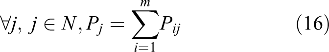
The objective function (1) is minimizing the makespan. Constraints (2) to (4) involve searching for and determining the job position. Constraint (5) indicates that the mth machine of the fth factory has the ability to process the $J_{j}$ . Constraint (6) ensures that the jobs are assigned to the factory, and it cannot be assigned to another factory. The maximum completion times of all jobs are compared by constraints (7) and (8). Constraints (9) and (10) determine the position of the job. Constraint (11) ensures that the robot transfers only one job at a time. Constraint (12) defines the completion time for job at position k on a machine. Constraint (13) indicates that the loading and unloading order of the job in the factory is determined according to the processing time of the job. Constraint (14) determines whether the robot is idle after one job is processed. The most common criterion for the optimal assessment is minimizing the maximum completion time. After the job processing sequence has been determined ( $π_{(j), i}$ , where the sequence is $π_{j}$ and the position of the job is j), the completion time is calculated by formula (15).

In addition, the corresponding formulas are shown in Table 2.

Table 2.

The corresponding formulas.

Objective:
$M i n C_{max} = max {C_{i} \| i = 1, 2,..., n}$		(1)
Subject to:
$\sum_{k = 1}^{n} X_{i, k} = 1$	$\forall i$	(2)
$\sum_{i = 1}^{n} X_{i, k} = 1$	$\forall k$	(3)
$\sum_{f = 1}^{f} Y_{k, f} = 1$	$\forall k$	(4)
$\sum_{f = 1}^{f} E_{j, m, f} = 1$	$\forall j, m, f > 0$	(5)
$(\sum_{j = 1}^{n} \sum_{m = 1}^{m} Z_{j, m, f}) = 1$	$f \in {1, 2, ..., f}$	(6)
$C_{max} \geq C k, m$	$\forall k, m$	(7)
$C_{k, m} \geq 0$	$\forall k, m$	(8)
$X_{i, k} \in {0, 1}$	$\forall i, k$	(9)
$Y_{k, f} \in {0, 1}$	$\forall k, f$	(10)
$(\sum_{m = 1}^{U} Z_{j, m}) = 1$	$j \in {1, 2, ..., n}; m \in {1, 2, ..., m}$	(11)
$C k, m \geq C_{l, m} + \sum_{i = 1}^{n} X_{i, k} = 1 \times P_{i, j} - B (1 - Y_{k, f}) - B (1 - Y_{l, f})$	$\forall k > 1, l < k, j, f$	(12)
$1 \times P_{i, j} - (3 - B \sum_{i = 1}^{n} X_{i, k} - U (1 - Y_{k, f}) - B (1 - Y_{m - 1, f})) \geq 0$	$\forall k > 1, i < k, j, f$	(13)
$1 \times P_{i, j} - (2 - U (1 - X_{i, k}) - B (1 - X_{i - 1, m})) \leq 1$	$\forall k > 1, i < k, j, m$	(14)
$C_{π (j), i} = max {C_{π (j), i} - 1, C_{π (j - 1), i}} + P_{π (j), i}$	$C_{π (j),0} = 0, C_{π (j), j} = 0, \forall i \in M, \forall j \in N$	(15)

Illustrative example

The 10 jobs are assigned to the three factories and each factory has a processing sequence for the jobs (Figure 1). Each factory has a robot that is responsible for transporting the jobs (Figure 2). Each job has a processing time, loading time, and unloading time. The processing time on the machine may differ for jobs. The time required by the robot to transport the job is ignored and the robot can only transport one job at the same time. The robot unloads the job and the robot requires a loading time to transport it to the next machine, after a job is completed on the previous machine. The longer the wait time of jobs, the longer the deterioration time. If the job is completed on two machines at the same time and the robot is idle, the robot randomly selects a machine to transport the processed job.

Figure 1.

The sequence of jobs in factories.

Figure 2.

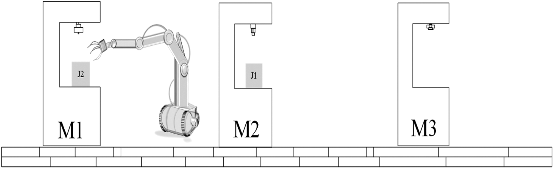
Illustrative example.

The transit time and the distances between the machines are negligible. An example was given to illustrate problem. The jobs are assigned to the factory F₁, then the processing sequence for M₁ is {1,2,3}, the processing sequence for M₂ is {1,2,3}, and the processing sequence for M₃ is {1,2,3}. As shown in Table 3, the time required for loading J₁ is 1 and its unloading time is 1. However, the processing completion time for J₁ on M₁ and the processing time for J₃ on M₃ are the same, and the transport of J₁ or J₃ for the robot is to judge.

Table 3.

The various time of jobs.

F₁	M ₁	M ₂	M ₃	$L_{j}$	$U_{j}$
J ₁	8	3	4	1	1
J ₂	4	6	5	1	2
J ₃	5	7	6	2	1

In addition, if the job has been processed and no robot can unload it, then the job will stay on the original machine for a waiting time. We objectively consider the green manufacturing process under the condition of deterioration time in jobs processing.

As shown in Figure 3, the whole path of the robot is given as follows

$L_{11} \to U_{11} \to L_{12} \to L_{21} \to U_{21} \to L_{31} \to U_{12} \to L_{22} \to L_{13} \to U_{31} \to U_{22} \to L_{32} \to U_{13} \to L_{23} \to U_{32} \to U_{23} \to L_{33} \to U_{33}$

Figure 3.

Gantt graph of problem description.

The canonical algorithm

The Nawaz-Enscore-Ham (NEH) variant used in most studies might not obtain new solutions that are better than the existing solutions,⁵² but it can still be accepted in probability in a similar manner to SA so the solutions in other regions can be explored.⁵³ Therefore, assigned jobs by the NEH strategy to each factory and obtained jobs sequence by the destruction and construction phases. The NEH heuristic algorithm or a variant of the NEH algorithm has been employed frequently to initialize the DPFSP when assigning factories to jobs.^53
–55 The NEH method can be described in the following steps. Finally, the SA algorithm is selected as the acceptance criterion.

(1) For each job compute the total processing time on m machines as follows

\forall j, j \in N, P_{j} = \sum_{i = 1}^{m} P_{i j}

(2) Next, the first operation is selected and evaluated for n jobs with the largest operation processing times.

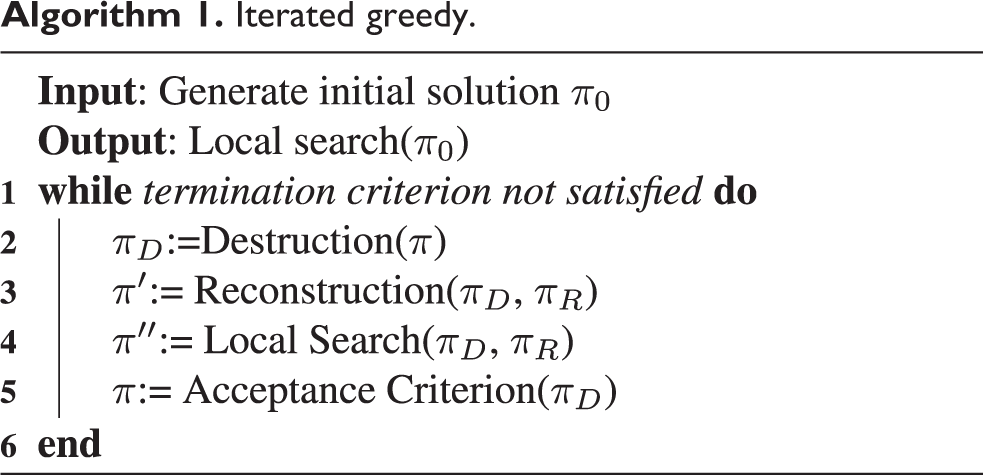
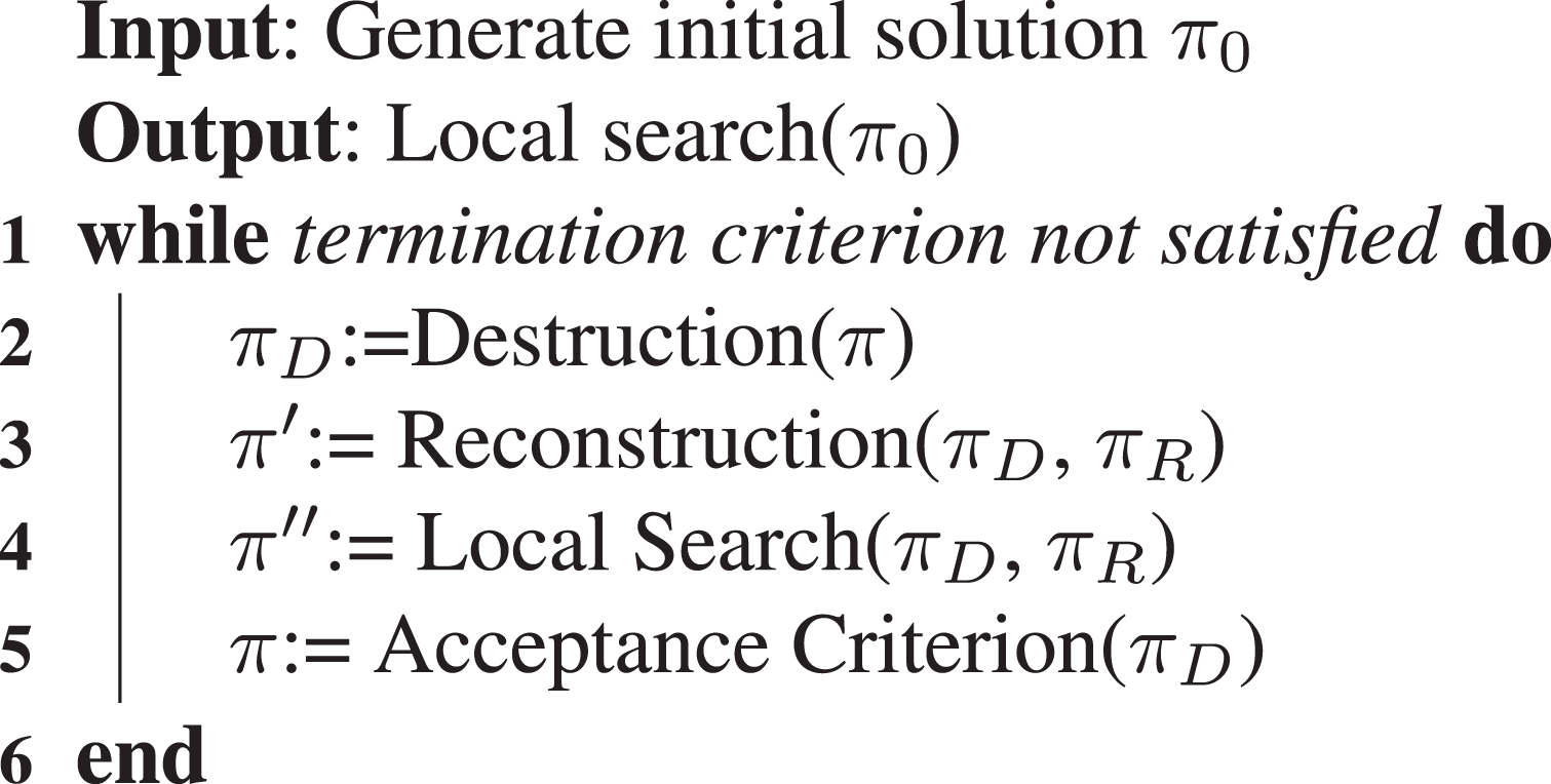
The IG algorithm was not applied to scheduling problems until its implementation was presented by Ruiz and Stützle.⁵⁶ IG is a simple stochastic metaheuristic algorithm, which starts with the initial solution and then improves the current solution by iterating in three main phases: destruction, construction, and acceptance phases.⁵⁷ Ruiz and Stützle⁵⁸ proposed a new IG algorithm, which they applied to randomly select d non-repetitive jobs from the sequence $π_{D}$ in the destruction phase. Pan and Ruiz⁵⁹ considered that d jobs are removed from π in the order that they are selected. The construction phase begins with the sequence $π_{D}$ and step d is performed, where the job in $π_{R}$ is reinserted into $π_{D}$ . The first job in $π_{R (1)}$ is inserted into all possible n − d + 1 positions in $π_{D}$ , and the best position in $π_{R (1)}$ is the best position for producing the minimum $C_{max}$ . Many studies have used the optimized or variable IG algorithm to solve scheduling problems.⁶⁰ The canonical framework of IG is given in Algorithm 1.

Algorithm 1

Iterated greedy.

The proposed algorithm

Framework of the proposed algorithm

In the proposed Algorithm 2, in the first stage, some elements are randomly removed from the current solution to obtain partial solutions. In the second stage, a greedy constructive heuristic method is used to reinsert the deleted elements to form a new complete solution. After the candidate solution is obtained, the acceptance criteria determine whether the new solution replaced the current solutions. To further improve the performance of the IIG algorithm, we add four kinds of neighborhood structures to generate new solutions, and use SA algorithm to jump out of the local optimal solution. Finally, the current solution is replaced by a better new solution.

Algorithm 2

Improved iterated greedy.

Problem encoding

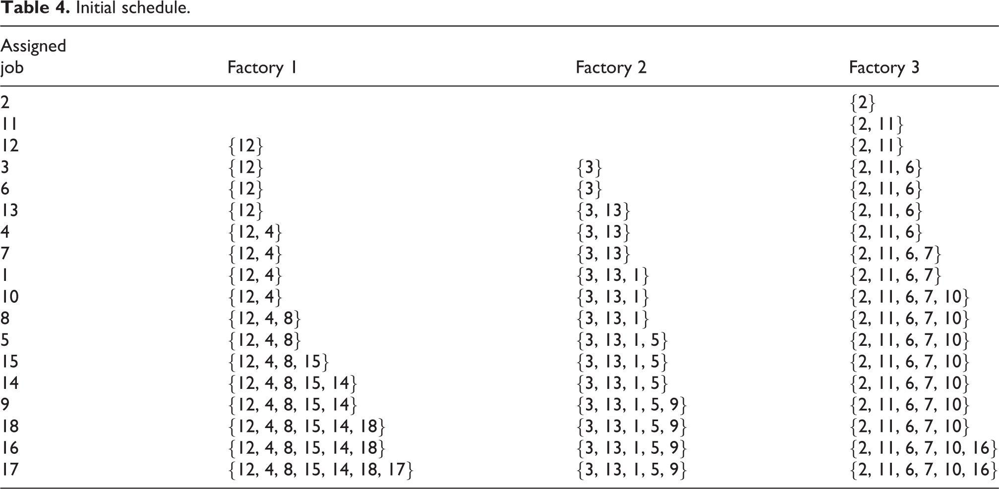
The jobs are scheduled and assigned to the factories randomly according to the NEH strategy (Table 4). Next, we consider the constraints on the problem where two vectors are utilized to encode the solution, that is, a two-dimensional (2-D) vector and a time matrix. To address the problem where the number of jobs is much larger than the number of factories, the jobs are randomly assigned to the factories. The first dimension of the 2-D vector is used to represent each factory and the second dimension represents each job that needs to be processed. The processing time, loading time, and unloading time of each job store in a 1-D vector, and the example is shown in Figure 4. Three factories each process six jobs. The processing sequence for a job in F₁ is {12,4,8,15,14,18,17} and that for a job in F₂ is {3,13,1,5,9}, and the job sequence in F₃ is {2,11,6,7,10,16}. The processing time of $J_{12}$ is 8, the loading time is 1, and the unloading time is 2, and the processing time of $J_{12}$ is 5, the loading time is 1, and the unloading time is 3.

Table 4.

Initial schedule.

Assigned job	Factory 1	Factory 2	Factory 3
2			{2}
11			{2, 11}
12	{12}		{2, 11}
3	{12}	{3}	{2, 11, 6}
6	{12}	{3}	{2, 11, 6}
13	{12}	{3, 13}	{2, 11, 6}
4	{12, 4}	{3, 13}	{2, 11, 6}
7	{12, 4}	{3, 13}	{2, 11, 6, 7}
1	{12, 4}	{3, 13, 1}	{2, 11, 6, 7}
10	{12, 4}	{3, 13, 1}	{2, 11, 6, 7, 10}
8	{12, 4, 8}	{3, 13, 1}	{2, 11, 6, 7, 10}
5	{12, 4, 8}	{3, 13, 1, 5}	{2, 11, 6, 7, 10}
15	{12, 4, 8, 15}	{3, 13, 1, 5}	{2, 11, 6, 7, 10}
14	{12, 4, 8, 15, 14}	{3, 13, 1, 5}	{2, 11, 6, 7, 10}
9	{12, 4, 8, 15, 14}	{3, 13, 1, 5, 9}	{2, 11, 6, 7, 10}
18	{12, 4, 8, 15, 14, 18}	{3, 13, 1, 5, 9}	{2, 11, 6, 7, 10}
16	{12, 4, 8, 15, 14, 18}	{3, 13, 1, 5, 9}	{2, 11, 6, 7, 10, 16}
17	{12, 4, 8, 15, 14, 18, 17}	{3, 13, 1, 5, 9}	{2, 11, 6, 7, 10, 16}

Figure 4.

Two-dimensional vector and one-dimensional vector.

Problem decoding

In the decoding, the 2-D vector is used for decoding, and we determine the corresponding positions for the jobs in the 2-D vectors according to the job number. Only one robot can transport each job and a block of time is available for a robot. A 2-D vector is needed to store each factory, the idle time of the robot, and one robot in each factory. If all of the jobs in a factory are deleted during the destruction phase in the IIG algorithm, the factory does not exist. We must assess whether the robot is transporting or not when a job is processed, as well as comparing the processing time after the robot loads or unloads the previous job. If the former is less than the latter, the job needs to continue to wait on the machine, and thus a waiting time and deteriorating time are considered, so the processing time period for the job is the exact time block available to the robot.

Each job number in the vector corresponds to the processing time, load time, and unload time for the jobs in the time matrix. The jobs may be processed at the same time on different machines. We need a strategy to solve the problem where two jobs finish at the same time and they must be transported by the robot. After a job has been processed, it is necessary to determine whether the robot is idle to obtain the entire path of the robot. Thus, on each machine, there is a time for unloading, another job, and a loading time after processing a job. If a job is processed, the robot will move to the current machine to load and unload the job. Robots cannot unload when they are loading. The deteriorating time is processing time multiplied by a coefficient so that some jobs have not only loading time and unloading time, waiting time, but also deteriorating time. The decoding heuristic is given in Algorithm 3.

Algorithm 3

Decoding heuristic.

Problem-specific neighboring structures

For solving the DPFSP, the neighborhood structures commonly used in the literature are insertion, such as insertion, swap, pairwise exchange, and variable neighborhood search algorithm.^61
–63 Considering the characteristics of the problem in this article and the development and exploration ability of the proposed algorithm, we propose four kinds of neighborhood structures, namely two kinds of insertion and two kinds of swap neighborhood structure, as given in Algorithm 4. In the neighborhood structures, we use two kinds of search operators, namely insertion operator and exchange operator. Considering the balance between the problem structure and the exploration and development ability, we will randomly select one of the four neighborhood structures for job scheduling in the RDPFSP. Algorithm 4 gives an example of neighborhood structure in local search, and Figure 5 shows four examples of neighborhood structure.

The first kind of insertion neighborhood structure: randomly select a factory, and randomly select two positions x and y from the job list, then insert the job of y position into the x position.

The second kind of insertion neighborhood structure: randomly select a job of a factory and insert it into a different factory, four kinds of insertion are as follows: (a) append to the last position of the new factory, (b) insert to the first position, (c) maintain the previous position, and (d) try to select a good position. Figure 5(b) shows one of the examples.

The first swap neighborhood structure: randomly select two positions x and y from the job list in a randomly selected factory and swap the two elements in the two positions.

The second swap neighborhood structure: randomly select two position x and y from the job list in two different factories, which are also randomly selected, and swap the two elements in the two positions.

Algorithm 4

Local search strategy.

Figure 5.

Four neighboring structures: (a) the first kind of insertion neighborhood structure, (b) the second kind of insertion neighborhood structure, (c) the second kind of swap neighborhood structure, and (d) the second kind of swap neighborhood structure.

From the steps of the four neighborhood structures presented in Algorithm 4, it is obvious that the time complexity of these structures are all of O(1). Therefore, the proposed neighborhood structures are simple and efficient.

Destruction heuristic

The random deletion of jobs from the generated sequence and the distributed sequence that was proposed by Tavares-Neto and Nagano.⁶⁴ Finally, the reconstruction phase is completed by applying the same insertion heuristic to the partial solution.

In the proposed IIG algorithm, the core phases are the destruction phase and the construction phase. These two phases optimize the solution by searching new regions in the solution space during each iteration. In the destruction phase, calculating the completion time for each factory by adding the time spent on jobs in each factory at first, where each job has a processing time on each machine and all of the jobs are distributed to each factory as shown in Figure 6(a).

Figure 6.

The destruction and construction phase: (a) the first kind of insertion neighborhood structure, (b) the second kind of insertion neighborhood structure, and (c) the second kind of swap neighborhood structure.

The strategy of destruction phase is conducted as follows. Calculate the maximum completion time for each factory and give priority to deleting the jobs from the factory with the largest $C_{max}$ . We randomly delete range of [d/2, d] jobs of selected factories. All of the jobs may even be deleted for a factory, then the equivalent of this factory has been deleted. A sequence of deleted jobs $D_{r}$ is then obtained. It is desirable to obtain a partial schedule that retains some of the characteristics of the schedule obtained in the previous iteration. Therefore, the solution is constructed incompletely.

Construction heuristic

In the construction phase, an example to illustrate how the construction phase starts with a partial plan is considered, before then reassigning one job at a time using greedy insert heuristics in Figure 6(b). Each job in the $D_{r}$ that deleted jobs during the destruction phase is tested at every position in all f factories, calculating the maximum completion time after inserting the job. After a job in $D_{r}$ is placed in the best position of the best factory (C _max increases to a minimum value), a new deletion sequence $D_{r}$ and job sequence of factory are generated, and the partial solution is updated. We continue to randomly select the next job in the $D_{r}$ and test the job at all positions in the factory to select the best position for insertion. The complete solution was not built until jobs of $D_{r}$ were reinserted into some of the solutions. Final position is the best position for inserting the job, so as to complete each factory almost have a minimum $C_{max}$ as shown in Figure 6(c).

Acceptance criterion

Acceptance criterion is able to avoid local best solutions, and thus random factors are introduced during the local search process. A worse solution than the current solution with a certain probability is accepted, so it is possible to escape from a local best solution and reach the global best solution. The SA algorithm is calculated according to Osman and Potts,⁶⁵ formula (17) is the method to calculate temperature, where T is an adjustable parameter. Ding et al.⁶⁶ explained the method of setting the initial temperature and cooling rate in formula (18), where $C_{max} (π)$ is the $C_{max}$ of sequence π of jobs, $C_{max} (π^{'})$ is the $C_{max}$ of sequence $π^{'}$ of a virtual job that processing time is 0

Temperature = T \cdot \frac{\sum_{i = 1}^{m} \sum_{j = 1}^{n} P_{i j}}{n \cdot m \cdot 10}

p = min {exp (\frac{C_{max} (π) - C_{max} (π^{'})}{T}),1}

SA starts at a relatively high temperature, before continuously decreasing the temperature parameter, where probability jump characteristics are also considered in the solution space to find the global optimization for the objective function. To avoid local optimization, we conduct global optimization according to the characteristics of the probability of escaping.

Experimental analyses

Experimental instances

In this article, to test the performance of the proposed IIG algorithm by solving robotic distributed flowshop problem, we randomly generated 20 instances according to the actual production data, where the test cases for the problem ranged in size between 20 and 500 jobs. The experimental instances comprised 20 instances denoted as “inst1” to “inst20.” The scale of the problem is as follows: (1) the number of factories is set to 2 and the number of machines is set to 3 for all the 20 instances, the number of jobs is different in each instance; (2) all of the jobs had a set of data that processing time and the processing time of each job is randomly generated in the range of [30, 50] in each instance; (3) each instance also included a set of data for each loading and unloading time, then the load time and unload time of jobs are randomly generated in the range of [0.5, 2]. The instances can be found in the website https://www.researchgate.net/publication/334735267_IJARS-realistic_instances.

Experimental parameter analysis

This section discusses the computational experiments used to evaluate the performance of the proposed algorithm. Our algorithm was implemented in C++ on an Intel Core i7 3.4-GHz PC with 16 GB of memory. To verify the effectiveness and efficiency of the proposed algorithm, after 30 independent runs, the resulting best solutions were collected for performance comparisons.

In the proposed algorithm, there are two main parameters as follows: (1) number of deleted jobs d, which determined the number of jobs deleted in the deletion phase; and (2) temperature T, that is, the temperature set in the acceptance criterion. Similar to Ruiz and Stützle,⁵⁶ in the proposed IIG algorithm, SA heuristic is also used for the acceptance criterion, and therefore to enhance the algorithm with the ability to escape from the local best solution. In this study, we also adapt a very simple constant temperature acceptance, as in the following formula (19), and T is a parameter and to be calibrated. According to many literatures and our detailed experimental comparisons, the two parameters are set as follows: d = 3 and T = 0.2

Temperature = \frac{T \cdot \sum_{k = 1}^{f} \sum_{j = 1}^{m} \sum_{i = 1}^{n} P_{i, j, k}}{n \cdot m \cdot f \cdot 10}

Efficiency of the local search

In the proposed algorithm, four neighborhood search strategies to enhance the search ability are proposed. To study the effectiveness of local search, we implement the IIG algorithm proposed in the “The canonical algorithm” section and the IIG without local search (IIG-NL) algorithm. The parameter settings of the two comparison algorithms are the same as the sections of experimental parameter analysis. The two comparative algorithms are tested with the same instance on the same PC. After 30 independent runs, the average results of each instance are collected and compared, as presented in Table 5. Table 5 records the data for the IIG and the IIG-NL algorithm. The last two columns give the percentage deviation obtained by the two algorithms, and the calculation formula is given as

dev = (f_{c} - f_{b}) / f_{b} \times 100 %

Table 5.

Comparison of best fitness between IIG and IIG-NL.^a

Instance	Best	Algorithm		Deviation
Instance	Best	IIG	IIG-NL	IIG	IIG-NL
Inst1	652.14	661.28	652.14	0.01	0.00
Inst2	957.83	960.40	957.83	0.27	0.00
Inst3	1632.76	1635.36	1632.76	0.16	0.00
Inst4	2665.31	2665.31	2693.84	0.00	1.07
Inst5	3462.90	3465.46	3462.90	0.07	0.00
Inst6	4394.45	4396.37	4394.45	0.04	0.00
Inst7	5873.79	5873.79	5901.20	0.00	0.47
Inst8	9082.24	9082.24	9135.97	0.00	0.59
Inst9	18242.10	18242.10	18548.40	0.00	1.68
Inst10	57754.10	57754.10	58928.10	0.00	2.03
Inst11	3949.35	3949.35	3962.62	0.00	0.34
Inst12	4421.03	4421.03	4440.89	0.00	0.45
Inst13	4896.54	4896.54	4913.33	0.00	0.34
Inst14	5390.29	5390.29	5391.73	0.00	0.03
Inst15	6054.09	6054.09	6054.44	0.00	0.01
Inst16	6540.84	6540.84	6568.14	0.00	0.42
Inst17	7018.35	7018.35	7062.90	0.00	0.63
Inst18	7760.69	7784.60	7760.69	0.31	0.00
Inst19	8395.56	8398.05	8395.56	0.03	0.00
Inst20	9071.09	9071.09	9085.74	0.00	0.42
mean	8410.77	8413.03	8497.18	0.11	0.42

IIG: improved iterated greedy; IIG-NL: IIG without local search.

^aThe best values are in bold.

The results in Table 5 can be summarized as follows: (1) IIG algorithm obtains 13 best solutions in a given 20 instances, while the IIG-NL algorithm obtains only 7 best solutions. (2) From the last two columns in Table 5, it can be seen that the average percentage of deviation obtained by the IIG algorithm is smaller than the IIG-NL algorithm. (3) Therefore, the performance of the proposed IIG algorithm is better than that of the IIG-NL algorithm.

To further test whether the differences in the above tables are significant, we have also made a detailed comparison, as shown in Figure 7. Figure 7 shows the fitness and 95% Fisher's Least Significant Difference (LSD) intervals from IIG and IIG-NL, and the p value = 0.0445. Obviously, IIG has a statistically significant advantage over the IIG-NL algorithm.

Figure 7.

Means and 95% LSD interval for the values of the two compared algorithms (p value = 0.0445).

Efficiency of the SA acceptance criterion

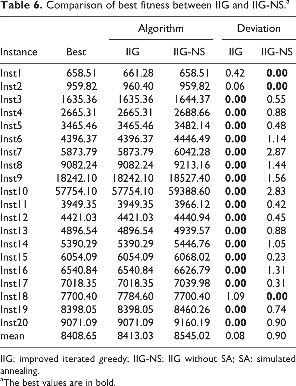
To study the effectiveness of the IIG algorithm, we implement the IIG algorithm proposed and the IIG without SA (IIG-NS) algorithm. The parameter settings of the two comparison algorithms are the same as the sections of experimental parameter analysis. The only difference between IIG and IIG-NS is that we use SA algorithm in the IIG algorithm proposed in this article; however, the IIG-NS algorithm does not use the SA algorithm when using the IIG algorithm to solve the problem. The two comparative algorithms are tested with the same instance on the same PC. After 30 independent runs, the average results of each instance are collected and compared, as shown in Table 6. In Table 6, the first column provides the name of the instance, and the second lists the best solution of the two algorithms. In the last two columns, the percentage deviation of the two algorithms is given, and the calculation formula is given in formula (20).

Table 6.

Comparison of best fitness between IIG and IIG-NS.^a

		Algorithm		Deviation
Instance	Best	IIG	IIG-NS	IIG	IIG-NS
Inst1	658.51	661.28	658.51	0.42	0.00
Inst2	959.82	960.40	959.82	0.06	0.00
Inst3	1635.36	1635.36	1644.37	0.00	0.55
Inst4	2665.31	2665.31	2688.66	0.00	0.88
Inst5	3465.46	3465.46	3482.14	0.00	0.48
Inst6	4396.37	4396.37	4446.49	0.00	1.14
Inst7	5873.79	5873.79	6042.28	0.00	2.87
Inst8	9082.24	9082.24	9213.16	0.00	1.44
Inst9	18242.10	18242.10	18527.40	0.00	1.56
Inst10	57754.10	57754.10	59388.60	0.00	2.83
Inst11	3949.35	3949.35	3966.12	0.00	0.42
Inst12	4421.03	4421.03	4440.94	0.00	0.45
Inst13	4896.54	4896.54	4939.57	0.00	0.88
Inst14	5390.29	5390.29	5446.76	0.00	1.05
Inst15	6054.09	6054.09	6068.02	0.00	0.23
Inst16	6540.84	6540.84	6626.79	0.00	1.31
Inst17	7018.35	7018.35	7039.98	0.00	0.31
Inst18	7700.40	7784.60	7700.40	1.09	0.00
Inst19	8398.05	8398.05	8460.26	0.00	0.74
Inst20	9071.09	9071.09	9160.19	0.00	0.90
mean	8408.65	8413.03	8545.02	0.08	0.90

IIG: improved iterated greedy; IIG-NS: IIG without SA; SA: simulated annealing.

^aThe best values are in bold.

The results in Table 6 can be summarized as follows: (1) IIG obtains 17 best solutions in a given 20 instances, while IIG-NS has 3 best solutions. (2) The percentage deviation of the two algorithms in the last two columns shows that the performance of IIG is better than IIF-NS.

To further test whether the differences in the above tables are significant, we have also made a detailed comparison, as shown in Figure 8. Figure 8 shows the fitness and 95% LSD intervals from IIG and IIG-NS, and the p value = 0.0001. Obviously, IIG has a statistically significant advantage over IIG-NS. The advantages of the SA algorithm are as follows: (1) avoid obtaining the local best solution and jump out of the local best solution to approach the global optimal solution, so as to improve the search ability; (2) the algorithm has a certain probability to accept the solution which is worse than the current solution, so it can jump out of the local optimal to a certain extent; (3) when the algorithm following into a local optimal, a SA-based heuristic is embedded and used to enhance the exploration abilities; (4) the algorithm broadens the search space.

Figure 8.

Means and 95% LSD interval for the values of the two compared algorithms (p value = 0.0001).

Comparisons with efficient algorithms

To verify the effectiveness of the IIG algorithm in solving the problems considered in this study, we compared its performance with the P-ABC, CABC, and TS algorithm. Numerous computational tests were conducted to compare the three algorithms. The four algorithms used the same encoding and decoding strategy, the same initialization function, and the same acceptance criteria. The comparison of the experimental images based on data showed that the proposed algorithm has obvious advantages compared with the other classical algorithms. The reliability of the four algorithms was tested by extending the RDPFSP instances. The fitness values obtained in the experiments are presented in Table 7. Table 7 contains 10 columns with the instance names in the first column. Data of the second column shows the best solution obtained for each instance. In the last four columns, the percentage deviation for each algorithm relative to the corresponding best solution is shown, which was calculated as the calculation formula (20).

Table 7.

Comparison of the best fitness with the different heuristics.^a

Instance	Best	Algorithm				Deviation
Instance	Best	IIG	IIG-NS	IIG	IIG-NS	TS	CABC	P-ABC	IIG
Inst1	654.72	654.72	664.81	657.49	661.28	0.00	1.54	0.42	0.01
Inst2	960.40	962.56	983.03	966.87	960.40	0.23	2.36	0.67	0.00
Inst3	1635.36	1651.00	1676.77	1637.47	1635.36	0.96	2.53	0.13	0.00
Inst4	2665.31	2719.64	2784.82	2683.51	2665.31	2.04	4.48	0.68	0.00
Inst5	3465.46	3506.00	3555.94	3471.27	3465.46	1.17	2.61	0.17	0.00
Inst6	4396.37	4465.00	4531.97	4425.93	4396.37	1.56	3.08	0.67	0.00
Inst7	5873.79	5947.09	6058.78	5892.67	5873.79	1.25	3.15	0.32	0.00
Inst8	9082.24	9249.00	9351.97	9125.53	9082.24	1.84	2.97	0.48	0.00
Inst9	18242.10	18479.90	18830.40	18493.70	18242.10	1.30	3.22	1.38	0.00
Inst10	57754.10	58939.00	58791.90	58524.60	57754.10	2.05	1.80	1.33	0.00
Inst11	3949.35	3987.60	4086.39	3958.81	3949.35	0.97	3.47	0.24	0.00
Inst12	4421.03	4461.18	4535.29	4484.54	4421.03	0.91	2.58	1.44	0.00
Inst13	4896.54	4971.42	5066.08	4912.32	4896.54	1.53	3.46	0.32	0.00
Inst14	5390.29	5458.76	5568.79	5416.73	5390.29	1.27	3.31	0.49	0.00
Inst15	6054.09	6120.59	6215.96	6090.70	6054.09	1.10	2.67	0.60	0.00
Inst16	6540.84	6650.75	6808.00	6573.02	6540.84	1.68	4.08	0.49	0.00
Inst17	7018.35	7140.40	7249.99	7062.63	7018.35	1.74	3.30	0.63	0.00
Inst18	7772.00	7799.00	7853.44	7772.00	7784.60	0.35	1.05	0.00	0.16
Inst19	8387.29	8501.00	8663.37	8387.29	8398.05	1.36	3.29	0.00	0.13
Inst20	9071.09	9207.97	9363.12	9138.24	9071.09	1.51	3.22	0.74	0.00
mean	8411.54	8543.63	8632.04	8483.77	8413.03	1.24	2.91	0.56	0.02

IIG: improved iterated greedy; IIG-NS: IIG without SA; SA: simulated annealing; CABC: cooperative artificial bee colony; TS: tabu search.

^aThe best values are in bold.

The results in Table 7 can be summarized as follows. (1) The P-ABC, CABC, and TS algorithm only calculated one best solution and the other best solutions were calculated by IIG. Compared with the P-ABC, CABC, and TS algorithms, the IIG algorithm obtained better results than the other three algorithms in terms of obtaining the best fitness value. (2) The average percentage deviation with the IIG algorithm was always less than the other three algorithms. Therefore, the results in Table 7 show that the performance of the proposed algorithm is better than that of other classical algorithms when solving the problem in this study.

To test whether there are significant differences between the four algorithms, we performed an analysis of variance, and the results are shown in Figure 9. Figure 9 shows that the performance of IIG of the four algorithms compared is significantly better than that of the other three algorithms.

Figure 9.

Results of comparison algorithms for comparisons with P-ABC, CABC, and TS. CABC: cooperative artificial bee colony; TS: tabu search.

In the next subsection, we analyze the reason why the IIG algorithm is better than the other efficient algorithms, such as P-ABC, CABC, and TS algorithms. IIG algorithm not only maintains the detection ability but also maintains the search ability.

We randomly selected eight instances of “Inst4, Inst6, Inst8, Inst13, Inst14, Inst15, Inst17, and Inst20.” Figure 10(a) to (h) records the convergence curves of these examples, showing the effectiveness of the proposed IIG algorithm. We can clearly see that in the convergence curve of each example, the IIG algorithm is the most effective.

Figure 10.

Convergence curve for instances: (a) Inst4, (b) Inst6, (c) Inst8, (d) Inst13, (e) Inst14, (f) Inst15, (g) Inst17, and (h) Inst20.

Figure 11 shows a Gantt chart of the processing time of the jobs in the two factories in the example, where each rectangle corresponds to one artifact. The jobs assigned to F₁ using the NEH strategy are {0, 1, 2, 12, 5, 6, 7, 11, 13, 15}, and the jobs assigned to F₂ are {4, 9, 10, 3, 14, 16, 17, 18, 19}. Take F₁ as an example, {0, 1, 2, 12, 5, 6, 7, 11, 13, 15} is the processing sequence of the jobs in F₁ on each machine. The robot transports J₀ to M₁ for processing. After the processing of J₀ is completed, the robot unloads J₀ from M₁ to M₂ for further processing, that is, operations path for robot transporting is $R_{m_{1}}^{J_{0}, m_{2}}$ . The J₁ processing on M₁ also needs to be unloaded by the robot, when the robot unloads the J₀ processed by M₂. At this time, the robot is on M₂, so the J₁ on M₁ produces the time to wait for the robot, waiting for the robot to unload J₀ and then unload J₁. As can be seen from Figure 11, the longer the waiting time, the longer the deterioration time.

Figure 11.

Gantt chart for the solution of the example.

Experiments analysis

Through the experimental comparisons, the proposed IIG algorithm shows significant better performance compared with other efficient algorithms. The main reasons that the IIG is superior to the other efficient algorithms, such as P-ABC, CABC, and TS algorithm, are as follows: (a) four neighborhood structures are presented to improve the exploitation abilities of the proposed algorithm; (b) when the algorithm following into a local optimal, an SA-based heuristic is embedded and used to enhance the exploration abilities; and (c) a problem-specific destruction and construction strategies are developed, which can further enhance the exploitation abilities.

Conclusion

In this study, we proposed an IIG algorithm to solve the problem that a robot is used to transport jobs in the DPFSP, where each factory has only one robot and the aim is to minimize the working time for the robot. In this problem, the robot must transfer each job from one machine to the next. The blocking constraint between the machines is considered, so it is necessary to determine whether the robot is idle when the job is completed. If the robot is not idle, the job will wait on the machine. The loading and unloading times are considered and different for all of the jobs conducted by the robot, and deteriorating time is also considered. Firstly, four types of neighborhood structures are developed in the proposed algorithm after studying the characteristics of the problem. Then, the SA algorithm is embedded in the proposed algorithm to enhance the exploration abilities. Furthermore, a problem-specific destruction and construction strategies are investigated. The ultimate objective is to minimize the makespan. We compared the performance of the proposed IIG algorithm in the test problem with three algorithms. The reliability and robustness of the IIG algorithm based on detailed experimental analyses was verified.

In the future research, we will investigate other scheduling methods for robots in various situations such as by (1) considering the scheduling of multi-robot cycle under the condition of saving energy consumption; (2) considering the situation where multiple robots handle the problem, where the objective is to minimize the number of robots used; and (3) considering other realistic application of robot green scheduling to improve the economic benefits.

Footnotes

Declaration of conflicting interests

The author(s) declared no potential conflicts of interest with respect to the research, authorship, and/or publication of this article.

Funding

The author(s) received no financial support for the research, authorship, and/or publication of this article.

ORCID iD

Junqing Li

References

Hou

, et al. Applications of artificial intelligence in intelligent manufacturing: a review. Front Inf Technol Electron Eng 2017; 18(1): 86–96.

Wang

Liu

. Underactuated robotics: a review. Int J Adv Robot Sys 2019; 16(4): 1–29.

Shao

Wang

, et al. Product environmental footprints assessment for product life cycle. J Clean Prod 2019; 233: 446–460.

Liu

Zeng

, et al. Product carbon footprint across sustainable supply chain. J Clean Prod 2019; 118320.

Naderi

Ruiz

. The distributed permutation flowshop scheduling problem. Comput Oper Res 2010; 37(4): 754–768.

Fernandez-Viagas

Framinan

. A bounded-search iterated greedy algorithm for the distributed permutation flowshop scheduling problem. Int J Prod Res 2015; 53(4): 1111–1123.

Zhang

Xing

Cao

. Scheduling distributed flowshops with flexible assembly and set-up time to minimise makespan. Int J Prod Res 2018; 56(9): 3226–3244.

Zhang

Xing

Cao

. Discrete differential evolution algorithm for distributed blocking flowshop scheduling with makespan criterion. Eng Appl Artif Intell 2018; 76: 96–107.

Chan

FTS

Chung

Chan

PLY

. An adaptive genetic algorithm with dominated genes for distributed scheduling problems. Exp Syst Appl 2005; 29(2): 364–371.

10.

Wang

Liu

, et al. An effective estimation of distribution algorithm for solving the distributed permutation flow-shop scheduling problem. Int J Prod Econ 2013; 145(1): 387–396.

11.

Bargaoui

Driss

Ghédira

. A novel chemical reaction optimization for the distributed permutation flowshop scheduling problem with makespan criterion. Comput Ind Eng 2017; 111: 239–250.

12.

Lin

Ying

. Minimizing makespan for solving the distributed no-wait flowshop scheduling problem. Comput Ind Eng 2016; 99: 202–209.

13.

Fernandez-Viagas

Perez-Gonzalez

Framinan

. The distributed permutation flow shop to minimise the total flowtime. Comput Ind Eng 2018; 118: 464–477.

14.

Wang

Zhou

, et al. A hybrid artificial bee colony algorithm for the fuzzy flexible job-shop scheduling problem. Int J Prod Res 2013; 51(12): 3593–3608.

15.

Pan

Tasgetiren

. A discrete artificial bee colony algorithm for the multi-objective flexible job-shop scheduling problem with maintenance activities. Appl Math Model 2014; 38(3): 1111–1132.

16.

Pan

Gao

. Pareto-based discrete artificial bee colony algorithm for multi-objective flexible job shop scheduling problems. Int J Adv Manuf Technol 2011; 55(9–12): 1159–1169.

17.

Liu

Zhang

A path planning approach for crowd evacuation in buildings based on improved artificial bee colony algorithm. Applied Soft Computing, 2018; 68: 360–376.

18.

Pan

Xie

. An effective shuffled frog-leaping algorithm for multi-objective flexible job shop scheduling problems. Appl Math Comput 2012; 218(18): 9353–9371.

19.

Song

Wang

, et al. Hybrid artificial bee colony algorithm for a parallel batching distributed flow shop problem with deteriorating jobs. IEEE Trans Cybern 2019. DOI: 10.1109/TCYB.2019.2943606.

20.

Gao

Chen

Deng

. An efficient tabu search algorithm for the distributed permutation flowshop scheduling problem. Int J Prod Res 2013; 51(3): 641–651.

21.

Chung

Chan

FTS

Chan

. A modified genetic algorithm approach for scheduling of perfect maintenance in distributed production scheduling. Eng Appl Artif Intell 2009; 22(7): 1005–1014.

22.

Naderi

Azab

. An improved model and novel simulated annealing for distributed job shop problems. Int J Adv Manuf Technol 2015; 81(1–4): 693–703.

23.

Lozano

Molina

Garc

. Iterated greedy for the maximum diversity problem. Eur J Oper Res 2011; 214(1): 31–38.

24.

Karabulut

. A hybrid iterated greedy algorithm for total tardiness minimization in permutation flowshops. Comput Ind Eng 2016; 98: 300–307.

25.

Takano

Nagano

. A branch-and-bound method to minimize the makespan in a permutation flow shop with blocking and setup times. Cogent Eng 2017; 4(1): 1389638.

26.

Ribas

Companys

Tort-Martorell

. An iterated greedy algorithm for solving the total tardiness parallel blocking flow shop scheduling problem. Exp Sys Appl 2019; 121: 347–361.

27.

Ruiz

Pan

Naderi

. Iterated greedy methods for the distributed permutation flowshop scheduling problem. Omega 2019; 83: 213–222.

28.

Pan

. An effective co-evolutionary artificial bee colony algorithm for steelmaking-continuous casting scheduling. Eur J Oper Res 2016; 250: 702–714.

29.

Tao

Jia

, et al. Efficient multi-objective algorithm for the lot-streaming hybrid flowshop with variable sub-lots. Swarm Evol Comput 2019.

30.

Deng

Wang

. A competitive memetic algorithm for multi-objective distributed permutation flow shop scheduling problem. Swarm Evol Comput 2017; 32: 121–131.

31.

Hou

Deng

, et al. Workspace analysis of a novel underactuated robot wrist based on virtual prototyping. Int J Adv Manuf Technol 2014; 72(1–4): 531–541.

32.

Dong

Ming

, et al. Design of open-closed-loop iterative learning control with variable stiffness for multiple flexible manipulator robot systems. IEEE Access 2019; 7: 23163–23168.

33.

Hurink

Knust

. A tabu search algorithm for scheduling a single robot in a job-shop environment. Discrete Appl Math 2002; 119(1–2): 181–203.

34.

Hurink

Knust

. Tabu search algorithms for job-shop problems with a single transport robot. Eur J Oper Res 2005; 162(1): 99–111.

35.

Arviv

Stern

Edan

. Collaborative reinforcement learning for a two-robot job transfer flow-shop scheduling problem. Int J Prod Res 2016; 54(4): 1196–1209.

36.

Che

Chu

. Multi-degree cyclic scheduling of two robots in a no-wait flowshop. IEEE Trans Autom Sci Eng 2005; 2(2): 173–183.

37.

Che

Chabrol

Gourgand

, et al. Scheduling multiple robots in a no-wait re-entrant robotic flowshop. Int J Prod Econ 2012; 135(1): 199–208.

38.

Che

Kats

Levner

. An efficient bicriteria algorithm for stable robotic flow shop scheduling. Eur J Oper Res 2017; 260(3): 964–971.

39.

Gultekin

Coban

Akhlaghi

. Cyclic scheduling of parts and robot moves in m-machine robotic cells. Comput Oper Res 2018; 90: 161–172.

40.

Kats

Levner

. A faster algorithm for 2-cyclic robotic scheduling with a fixed robot route and interval processing times. Eur J Oper Res 2011; 209(1): 51–56.

41.

Nouri

Driss

Ghédira

. Simultaneous scheduling of machines and transport robots in flexible job shop environment using hybrid metaheuristics based on clustered holonic multiagent model. Comput Ind Eng 2016; 102: 488–501.

42.

Nouri

Driss

Ghédira

. Hybrid metaheuristics for scheduling of machines and transport robots in job shop environment. Appl Intell 2016; 45(3): 808–828.

43.

Zabihzadeh

Rezaeian

. Two meta-heuristic algorithms for flexible flow shop scheduling problem with robotic transportation and release time. Appl Soft Comput 2016; 40: 319–330.

44.

Elmi

Topaloglu

. A scheduling problem in blocking hybrid flow shop robotic cells with multiple robots. Comput Oper Res 2013; 40(10): 2543–2555.

45.

Elmi

Topaloglu

. Scheduling multiple parts in hybrid flow shop robotic cells served by a single robot. Int J Comput Integr Manuf 2014; 27(12): 1144–1159.

46.

Chen

Zhang

, et al. Hybrid chaos-based particle swarm optimization-ant colony optimization algorithm with asynchronous pheromone updating strategy for path planning of landfill inspection robots. Int J Adv Robot Syst 2019; 16(4): 1729881419859083.

47.

Chen

Mao

Yang

, et al. Cost-efficient inter-robot delivery for resource-constrained and interdependent multi-robot schedules. Int J Adv Robot Syst 2019; 16(1): 1729881419828049.

48.

Lee

Yeh

Chung

. Total tardiness minimization in permutation flowshop with deterioration consideration. Appl Math Model 2014; 38(13): 3081–3092.

49.

Cheng

Tadikamalla

Shang

, et al. Bicriteria hierarchical optimization of two-machine flow shop scheduling problem with time-dependent deteriorating jobs. Eur J Oper Res 2014; 234(3): 650–657.

50.

. Research on no-idle permutation flowshop scheduling with time-dependent learning effect and deteriorating jobs. Appl Math Model 2016; 40(4): 3447–3450.

51.

Bai

Duan

, et al. An improved artificial bee colony algorithm for addressing distributed flow shop with distance coefficient in a prefabricated system. Int J Prod Res 2019: 1–21. DOI: 10.1080/00207543.2019.1571687.

52.

Nawaz

Enscore

Jr Ham

. A heuristic algorithm for the m-machine, n-job flow-shop sequencing problem. Omega 1983; 11(1): 91–95.

53.

Fernandez-Viagas

Valente

Framinan

. Iterated-greedy-based algorithms with beam search initialization for the permutation flowshop to minimise total tardiness. Exp Syst Appl 2018; 94: 58–69.

54.

Taillard

. Some efficient heuristic methods for the flow shop sequencing problem. Eur J Oper Res 1990; 47(1): 65–74.

55.

Hatami

Ruiz

Andrés-Romano

. Heuristics and metaheuristics for the distributed assembly permutation flowshop scheduling problem with sequence dependent setup times. Int J Prod Econ 2015; 169: 76–88.

56.

Ruiz

Stützle

. A simple and effective iterated greedy algorithm for the permutation flowshop scheduling problem. Eur J Oper Res 2007; 177(3): 2033–2049.

57.

Arroyo

JEC

Leung

JYT

Tavares

. An iterated greedy algorithm for total flow time minimization in unrelated parallel batch machines with unequal job release times. Eng Appl Artif Intell 2019; 77: 239–254.

58.

Ruiz

Stützle

. An iterated greedy heuristic for the sequence dependent setup times flowshop problem with makespan and weighted tardiness objectives. Eur J Oper Res 2008; 187(3): 1143–1159.

59.

Pan

Ruiz

. An effective iterated greedy algorithm for the mixed no-idle permutation flowshop scheduling problem. Omega 2014; 44: 41–50.

60.

Karabulut

Tasgetiren

. A variable iterated greedy algorithm for the traveling salesman problem with time windows. Inf Sci 2014; 279: 383–395.

61.

Pan

Mao

. A discrete teaching-learning-based optimisation algorithm for realistic flowshop rescheduling problems. Eng Appl Artif Intell 2015; 37(1): 279–292.

62.

Rifai

Nguyen

Dawal

SZM

. Multi-objective adaptive large neighborhood search for distributed reentrant permutation flow shop scheduling. Appl Soft Comput 2016; 40: 42–57.

63.

Pan

Gao

XinYu

, et al. Effective constructive heuristics and metaheuristics for the distributed assembly permutation flowshop scheduling problem. Appl Soft Comput 2019; 81: 105492.

64.

Tavares-Neto

Nagano

. An iterated greedy approach to integrate production by multiple parallel machines and distribution by a single capacitated vehicle. Swarm Evol Comput 2019; 44: 612–621.

65.

Osman

Potts

. Simulated annealing for permutation flow-shop scheduling. Omega 1989; 17(6): 551–557.

66.

Ding

Song

Gupta

, et al. An improved iterated greedy algorithm with a Tabu-based reconstruction strategy for the no-wait flowshop scheduling problem. Appl Soft Comput 2015; 30: 604–613.

Solving robotic distributed flowshop problem using an improved iterated greedy algorithm

Abstract

Keywords

Introduction

Problem formulation

Problem description

Problem model

Illustrative example

The canonical algorithm

The proposed algorithm

Framework of the proposed algorithm

Problem encoding

Problem decoding

Problem-specific neighboring structures

Destruction heuristic

Construction heuristic

Acceptance criterion

Experimental analyses

Experimental instances

Experimental parameter analysis

Efficiency of the local search

Efficiency of the SA acceptance criterion

Comparisons with efficient algorithms

Experiments analysis

Conclusion

Footnotes

Declaration of conflicting interests

Funding

ORCID iD

References