Linear model predictive control of automatic parking path tracking with soft constraints

Abstract

This study examines how to improve the accuracy of auto parking path tracking control; therefore, a linear model predictive control with softening constraints path tracking control strategy is proposed. Firstly, a linear time-varying predictive model of vehicle is established, and the future state of the vehicle can be predicted. The designed objective function fully considers the deviation between the predictor variable and the reference variable. Also, the relaxation factors are added to the optimization process, and the control increment of each cycle is calculated by the quadratic programming. Through rolling optimization and feedback correction, all kinds of deviations in the control process can be corrected in time. Then, the Simulink/CarSim simulation is carried out jointly. Furthermore, the path tracking simulation based on proportion–integration–differentiation control and no control is also carried out to compare with the model predictive control. Finally, a real vehicle test is carried out for model predictive control algorithm, and a comparative experiment based on proportion–integration–differentiation control and no control is carried out.

Introduction

The automatic parking system (APS) is one of the advanced driver assistant systems (ADAS). Its role is to assist drivers to realize parking safely and quickly, which can reduce the requirements of the driver’s skill and accidents caused by human factors such as vehicle collision. The ADAS technologies usually comprise three steps: the detection, the decision, and the control. ^{1 –4} Similarly, the APS mainly consists of three parts: environment perception, path planning, ⁵ and path tracking. ^6,7 The architecture of APS is shown in Figure 1. The APS controller obtains the information of parking slot and obstacles through the environmental perception section which includes various sensors, such as ultrasonic sensors, camera, wheel speed sensor, and steering angle sensor (Part I in Figure 1). The sensors measure the distance between the car and the obstacles, the real-time visual data, the current car velocity, and the steering angle for further process. It will be decided via multi-sensor data fusion whether the parking slot is available. Meanwhile, the world coordinate system is created and the start position of the car is estimated (Part II, a). The system will generate the parking trajectory using a particular algorithm after the slot is decided (Part II, b). Based on the designed trajectory, the path tracking controller can control the steering wheel, throttle, and brake to decide the parking maneuver (Part II, c). The real-time position of the vehicle is estimated via velocity and steering angle measured by the wheel speed sensor and steering wheel sensor, respectively.

Figure 1.

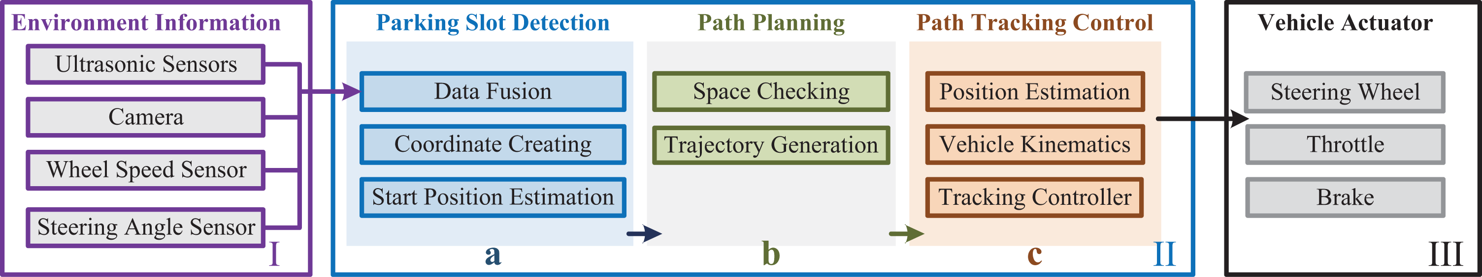
Architecture of automatic parking system.

Path planning and path tracking control complement each other. Path tracking control algorithm is one of the key technologies of APS. The major problems of parking path tracking control include ensuring the accuracy of path tracking, the ride comfort of vehicle navigation, the position and orientation of the vehicle when it finishes parking maneuver. As one of the critical problems of automatic parking technology, a large number of scholars have proposed the related control algorithms. Hua et al. ⁸ suggested an automatic parking path control method considering time delay, which solved the problem of the traditional APS control model not regarding vehicle control delay. Oetiker et al. ⁹ put forward a semi-automatic parking assistant system based on navigation area, which is able to perceive environment information in real time via the environment perceptual sensing device and optimize parking routes to avoid collisions. Demirli et al. ¹⁰ designed an Adaptive Neuro-Fuzzy Inference System. The vehicle does not need to know the desired polynomial path to track, but it will approximate such a way by knowing only the start configuration. Huang et al. ¹¹ proposed a model-free intelligent, self-organizing fuzzy controller for parking path tracking. This intelligent controller has a system-learning mechanism without expert knowledge or a trial-and-error process. The algorithms above is able to track the existing path. However, the current control cannot be optimized according to the changing trend of the parking path in the whole process. Besides, the control of steering wheel and speed are relatively independent. In other words, they are not organic combination during the parking process. As a result, the speed and steering wheel control will be uncoordinated. In addition, there will be adverse effects on the accuracy of path tracking.

Compared with existing algorithms, the model predictive control (MPC) method is capable of optimizing the current control according to the trend of the reference parking path. Besides, the control of steering wheel and speed are of organic combination and coordination. In addition, it has beneficial effects on the accuracy of path tracking. MPC was proposed in the 1970s. It is an advanced control method which is usually used to control a process with constraints. It is a heuristic control algorithm applied in the industrial process and has rich theoretical and practical contents. ^{12 –14} Model predictive controllers depend on models of the process, which are often linear models. There should be desirable properties of approximation accuracy, physical interpretation, suitability for control and easiness of development for a good model. ¹⁵ The most prominent attraction of MPC is that it can handle constraints explicitly. ^16,17 In other words, by predicting the future state of the system and adding constraints to the future input, output, or state variables, the constraints are expressed in an online solving quadratic programming (QP) or nonlinear programming problem. The MPC optimization problem could be solved when the feasible set (the set of possible solutions) is not empty. If the set is not empty, the feasible set may be reduced by any constraints imposed on the manipulated variables. However, depending on the current operating point of the process, unmeasured variables, the model-process mismatch, and existing input constraints, the feasible set of the MPC optimization problem may be empty. ¹⁸ Adding relaxation factors to the constraints (soft constraints) is a good idea. ¹⁹ This method is assumed that the predicted control variables is able to temporarily violate the original hard constraints, which enforces the existing feasible set. The optimization problem is solved online. The essential features of MPC are prediction model, rolling optimization, and feedback correction. MPC is a typical approach in industrial advanced control. It has been widely used in various of domain, such as supply chain management in semiconductor manufacturing, ²⁰ application to autoclave composite processing, ²¹ energy efficiency control in buildings, ²² integrated wastewater treatment systems, ²³ flight control, ²⁴ magnetic spacecraft attitude control, ²⁵ and so on. Moreover, there are many applications of MPC in vehicle control, such as the active front steering, ^{26 –29} automatic vehicle longitudinal control, ³⁰ vehicular adaptive cruise control, ³¹ vehicle yaw and lateral stability control, ³² automatic vehicle braking, and steering control. ³³ It also can efficiently handle multiple optimization objectives and system constraints. Besides, it can make up the model mismatch, time-varying, and interference caused by uncertainty. Hence it is suitable for path tracking control of a vehicle.

Hence, in this article, the parking path is planned based on the vehicle kinematics model, and an automatic parking path tracking based on MPC with soft constraints is proposed. The MPC parking controller controls the speed and the front wheel steering coordinately. It can predict the current control volume according to the change of parking path in the future period so that the speed and steering wheel can be controlled in phase, and the path tracking is of high accuracy.

Parking path planning and simulation

Vehicle kinematics model

Automatic parking is a low-speed process, ⁹ and the speed is less than 3 m·s⁻¹. Considering the comfort of the passengers, ³⁴ the acceleration is usually less than 2.5 m·s⁻². Assuming that the parking conditions are right, ignoring the dynamic characteristics of vehicles, only considering the motion characteristics of vehicles, when the steering wheel meets the Ackerman angle constraint, the front wheel steering angle can be expressed by an angle δ. The kinematic equation of vehicle can be obtained as follows

$\left[\begin{array}{c}\dot{x}\\ \dot{y}\\ \dot{\phi }\end{array}\right]=\left[\begin{array}{cc}\text{cos}\phi & 0\\ \text{sin}\phi & 0\\ \text{tan}\delta /L& 0\end{array}\right]\left[\begin{array}{c}v\\ \delta \end{array}\right]$

1

where v denotes the longitudinal velocity of the vehicle. There (x, y) are the coordinates of O_r which is the midpoint of the rear axle in a Euclidean reference frame. The heading angle of the vehicle is φ. The wheelbase of a vehicle is L.

Figure 2 is a schematic diagram of a vehicle kinematics model, in which the rectangular β represents the vehicle coverage area, where W is the width of a vehicle, δ is the front wheel steering angle, v denotes the longitudinal velocity of the vehicle, L is wheelbase of a vehicle, φ is the heading angle, O_r the midpoint of the vehicle rear axle, L_f and L_r are the length of the front and rear suspension, respectively. Additional, XOY is the world coordinate system.

Figure 2.

Vehicle kinematics model.

Parking path planning

Parking path planning can be divided into three steps:

Determine the minimum length of parking slot L_{p min} based on the geometric parameters of a vehicle.

Detecting obstacles in parking by environmental sensing sensors and determining the actual length of the parking slot L_p . Proceeding to next step when L_p ≥ L_{p min}.

The path planning is carried out according to the actual length of the parking slot and the parameters of the car body.

As shown in Figure 3 is a typical parallel parking scenario. The vehicle usually reverse into the parking slot during parallel parking process. More specifically, the parking process can be divided into three parts, including the acceleration stage, the constant speed stage, and the deceleration stage. ³⁵ The vehicle must avoid collisions with the obstacles in any direction during parking process. ³⁶ The distance between any point of the car and obstacle cannot be less than safety distance: ΔS, which is to ensure maneuvering safety. The safety distance in the parking process is defined as ΔS. There are three situations where collisions are easy to occur during the parking process. Firstly, during the parking maneuver, the vehicle should not exceed the road axis so as to avoid collision with the opposite vehicle. Secondly, the safety distance between the vehicle and the obstacle 2 should be kept to avoid collision. Finally, at the end of parking, vehicle should keep safety distance with obstacle 1 to avoid collision. These conditions must be taken into full consideration when plan the path.

Figure 3.

Typical parallel parking scenario.

As shown in Figure 4, the vehicle will reverse into the parking slot through the path $\overline{ABCO}$ . The size of the vehicle and the parking slot are in the same order of magnitude, so the vehicle cannot be treated as a particle during parking maneuvers. The desired parking result requires that the midpoint of the vehicle rear axle O_r coincides with the original point O, the heading angle is 0° in the world coordinate system XOY, and the left side of the vehicle is flat on the left side of the obstacle 1 and 2, respectively.

Figure 4.

Geometric relationship of parking path planning.

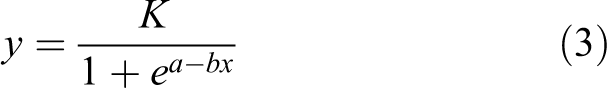
In this article, a smooth connected parallel parking path is designed considering the conditions of the small parking slot and narrow lateral width. As shown in Figure 4, the parking trajectory is composed of three horizontal connected line segments. The line segments are $\overline{AB}$ , $\overline{BC}$ , and $\overline{CO}$ . The point A is the start position of the vehicle. The segment $\overline{CO}$ is a circular arc with the center of O ₁(0, R ₁), where O ₁ is on the Y-axis and R ₁ is the turning radius of the vehicle. The segment $\overline{BC}$ is a straight line that is tangent to $\overline{CO}$ and $\overline{AB}$ , with a length of L_BC and a slope of θ. It can be obtained

$\{\begin{array}{l}{x}_C=R_1\text{sin}\theta \\ y_C=R_1(1-\text{cos}\theta )\\ x_B=x_C+L_{BC}\text{cos}\theta \\ y_B=y_C+L_{BC}\text{sin}\theta \end{array}$

2

where (x_B , y_B ) and (x_C , y_C ) is the coordinate of points B and C in the world coordinate system XOY, respectively.

To ensure safety, the curve segment $\overline{AB}$ is generated by the following equation

$y=\frac{K}{1+e^{a-bx}}$

3

where $e=\underset{n\to \infty }{{\displaystyle \text{lim}}}{(1+\frac{1}{n})}^n$ is the nature base and K, a, and b are constants. The point B determines the position of the segment, and at the point B, it conforms to ${\ddot{y}|}_{x=x_B}=0$ . So, the constants above are obtained

$\{\begin{array}{l}a-b{x}_B=0\\ K=2y_B\\ \text{tan}\theta =Kb/4\end{array}$

4

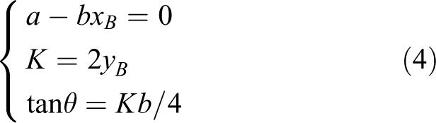
From the equations (2) and (4), it is known that the parking path can be determined entirely by the parameters R ₁, θ, and L_BC .

Parking path simulation

Vehicle parking is a relatively fixed process, and the optimal path can be generated off-line according to the length of the different parking slot. Due to the different geometric parameter of vehicles, the optimal parking path is different in the same parking slot. In this article, the generation of the parking path is based on the parameters of an sport utility vehicle (SUV), and the specific parameters of the vehicle are shown in Table 1.

Table 1.

Parameters of the test vehicle.

Parameters	Values
L	2.807 m
W	1.893 m
Lf	0.912 m
Lr	0.912 m
δ max	39.67°

To protect the vehicle performance, it is essential to avoid the front wheel at the maximum angle. The minimum radius of the planned parking path is as follows

$R_{\text{min}}=\frac{L}{\text{tan}({\delta }_{\text{max}}/1.1)}$

Vehicle parking requires that the narrower the parking slot, the better. Taking ΔS = 0.3 m, according to the path planning method mentioned above, we carried out a path planning simulation, and it is shown in Figure 5. The minimum length of the parking slot is L_{p min} = 6.9 m, and the corresponding parking path parameters are R ₁ = R _min = 3.855 m, θ = 0.52 rad, and L_BC = 1.54 m. The origin is set as the starting point of the path by coordinate transformation to facilitate path tracking control simulation.

Figure 5.

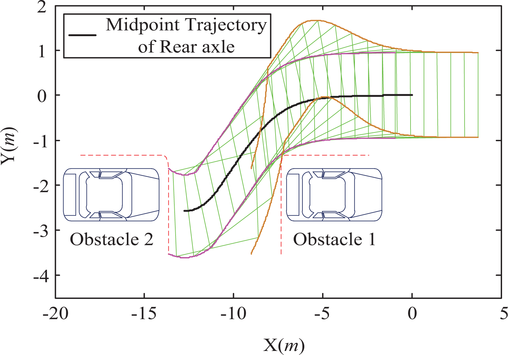
Simulation of parking path planning.

Design of automatic parking controller

The process of parking path tracking control is tracking a series of sampling points one by one on the reference path that is well planned, and point set P_{r set} represents all the sampling points of reference path. Automatic parking control strategy is shown in Figure 6. In the parking process, the algorithm needs several steps to implement. Firstly, the controller obtains current state of the vehicle in real time via various of sensors and the vehicle state can be expressed by state vector χ. Secondly, combining with the last time control variable and the reference path point, the output state of Y in the future for a period can be predicted. Thirdly, the control increment can be obtained by the optimization of QP with softening constraints. Finally, the current control variable u can be obtained with the latest control variable and the current control increment. The method of rolling optimization is used to calculate the latest control variable for path tracking until the end of parking.

Figure 6.

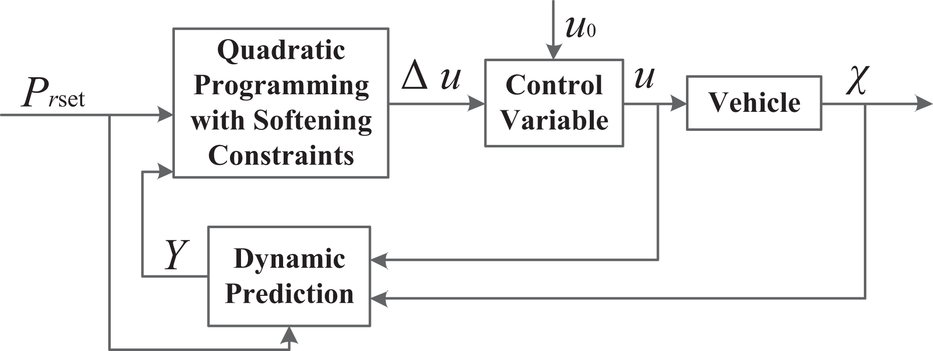
Automatic parking control strategy based on MPC with soft constraints. MPC: model predictive control.

Discretization of vehicle kinematic model

The kinematic model of the vehicle is a linear time-varying model. The kinematic equation of the car is discretized to facilitate the design of the controller. Defining vectors χ = [x, y, φ]^T, u = [v, δ]^T, the equation (1) can be expressed as

$\dot{\chi }=f(\chi ,u)$

5

The equation (5) is carried out at the reference point [χ_r , u_r ], and the higher order is eliminated

$\dot{\chi }=f({\chi }_r,u_r)+A(\chi -{\chi }_r)+B(u-u_r)$

6

In the form, A and B are the Jacobi matrices of f(χ, u) relative to vectors χ and u, respectively.

For

${\dot{\chi }}_r=f({\chi }_r,u_r)$

7

The equation (6) subtract equation (7) and then discrete and reorganize. The following equations can be obtained

$\{\begin{array}{c}\chi (k+1)=A_k\chi (k)+B_{k}u(k)+\text{g}(k)\\ \eta (k)=C\chi (k)\end{array}$

8

where

$\{\begin{array}{l}{A}_k=\left[\begin{array}{ccc}1& 0& -v_r(k)\text{sin}{\phi }_r(k)T\\ 0& 1& v_r(k)\text{cos}{\phi }_r(k)T\\ 0& 0& 1\end{array}\right]\\ \text{g}(k)={\chi }_r(k+1)-A_k{\chi }_r(k)-B_k{u}_r(k)\\ B_k=\left[\begin{array}{cc}\text{cos}{\phi }_r(k)T& 0\\ \text{sin}{\phi }_r(k)T& 0\\ \text{tan}{\delta }_r(k)T/L& \left(v_r(k)T\right)/\left(L{\text{cos}}^2{\delta }_r(k)\right)\end{array}\right]\end{array}$

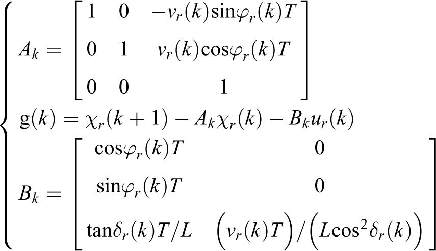
In which *(k) represents the state and control variable of the system at the k sampling time. The * _k represents the state matrix and the control variable matrix corresponding to the k sampling time, and the * _r represents the reference variable. T is the sampling period and vector C = diag(1, 1, 1).

Due to the limitation of the mechanical structure and physical conditions, the control variable and control increment within the sampling period must satisfy the following constraints:

$\{\begin{array}{l}△u_{\text{min}}\le △u\le △u_{\text{max}}\\ u_{\text{min}}\le u\le u_{\text{max}}\end{array}$

9

where the Δu is the control increment vector. The Δu _min and Δu _max are the lower and upper limit of the control increment vector in the sampling period, respectively. The u _min is the minimum control variable vector, and the u _max is the maximum control variable vector.

Dynamic prediction of vehicle’s future state

Due to the constraint condition of control increment in the sampling period, we can introduce the control increment to the optimization method to restrict it. The new state space equation can be taken as follows

$\xi (k)=\left[\begin{array}{c}\chi (k)\\ u(k-1)\end{array}\right]$

10

By considering equations (8) and (10), it can be obtained

$\{\begin{array}{l}\xi (k+1)={\overline{A}}_k\xi (k)+{\overline{B}}_k△u(k)+{\overline{g}}_k\\ \overline{\eta }(k)=\overline{C}\xi (k)\end{array}$

11

where

$\{\begin{array}{c}{\overline{A}}_k=\left[\begin{array}{cc}{A}_k& B_k\\ 0& I\end{array}\right],{\overline{B}}_k=\left[\begin{array}{c}{B}_k\\ I\end{array}\right]\\ \overline{C}=\left[\begin{array}{cc}C& 0\end{array}\right],\overline{g}(k)=\left[\begin{array}{c}g(k)\\ 0\end{array}\right]\end{array}$

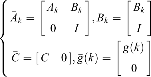
and the I is the unit matrix.

Due to the time-varying factor in equation (11), the time-varying MPC is difficult to meet the real-time requirements of the controller, and it will lead to complex nonlinear constraints. ³⁷ To simplify the calculation, the following assumptions are made

$\{\begin{array}{l}{A}_{k+i,k}=A_k\\ B_{k+i,k}=B_k\end{array}$

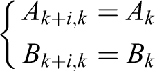
where * _{k+i ,k} represents the prediction matrix of the k+i sampling time at the k sampling time and i = 1,2,….

At sample time k, after predicting the output value in the future for N_p sampling time and the control increment for N_c sampling time, the output of the system in the future sampling time is expressed in matrix form

$Y(k)={\psi }_k\xi (k)+{\Theta }_k\Delta U(k)+{\Phi }_{k}G(k)$

12

where

$\begin{array}{l}Y\left(k\right)=\left[\begin{array}{c}\overline{\eta }\left(k+1|k\right)\\ \cdots \\ \overline{\eta }\left(k+N_p|k\right)\end{array}\right],△U(k)=\left[\begin{array}{c}△u(k|k)\\ \cdots \\ △u(k+N_c-1|k)\end{array}\right],{\Phi }_k=\left[\begin{array}{cccc}\overline{C}& 0& \cdots & 0\\ \overline{C}{\overline{A}}_k& \overline{C}& \cdots & 0\\ ⋮& ⋮& & ⋮\\ \overline{C}{\overline{A}}_k^{N_p-1}& \overline{C}{\overline{A}}_k^{N_p-2}& \cdots & \overline{C}\end{array}\right],{\psi }_k=\left[\begin{array}{c}\overline{C}{\overline{A}}_k\\ \cdots \\ \overline{C}{\overline{A}}_k^{N_p}\end{array}\right]\\ {\Theta }_k\text{=}\left[\begin{array}{cccc}\overline{C}{\overline{B}}_k& 0& \cdots & 0\\ \overline{C}{\overline{A}}_k{\overline{B}}_k& \overline{C}{\overline{B}}_k& \cdots & 0\\ ⋮& ⋮& & ⋮\\ \overline{C}{\overline{A}}_k^{N_p-1}{\overline{B}}_k& \overline{C}{\overline{A}}_k^{N_p-2}{\overline{B}}_k& \cdots & \overline{C}{\overline{A}}_k^{N_p-N_c-1}{\overline{B}}_k\end{array}\right],G(k)=\left[\begin{array}{c}\overline{g}(k|k)\\ \cdots \\ \overline{g}(k+N_p-1|k)\end{array}\right]\end{array}$

where *(k+i|k) represents the predicted value of the k+i sampling time at k sampling time. The corresponding reference output is

$Y_r(k)=\left[\begin{array}{c}{\eta }_r(k+1|k)\\ \mathrm{...}\\ {\eta }_r(k+N_p|k)\end{array}\right]$

13

Optimization of control increment based on QP with soft constraints

The relaxation factor is added to the constraint condition to make the vehicle track the path well and prevent the infeasible solution in the process of solving. ¹⁹ The following objective function is used

$J(k)={\Vert Y(k)-Y_r(k)\Vert }_Q^2+{\Vert \Delta U(k)\Vert }_R^2+{\Vert U\left(k\right)-U_r\left(k\right)\Vert }_F^2+{\Vert \epsilon \Vert }_{\rho }^2$

14

where

${\Vert \ast \Vert }_{\text{Matrix}}^2={\ast }^T\text{Matrix}\ast$

Matrix Q is the weight matrix of prediction deviation. Matrix R is the weight matrix of the predictive control increment. Matrix F is the weight matrix of the deviation of the predictive control variable. The parameter ε = [ε ₁, ε ₂, ε ₃, ε ₄]^T is the vector of the relaxation factor. The parameter ρ is the weight matrix of relaxation factor

$U_r\left(k\right)=\left[\begin{array}{c}{u}_r(k|k)\\ \cdots \\ u_r(k+N_c-1|k)\end{array}\right],U\left(k\right)=\left[\begin{array}{c}u(k|k)\\ \cdots \\ u(k+N_c-1|k)\end{array}\right]$

By considering equations (9) and (14), it can be obtained

$\{\begin{array}{l}△u_{\text{min}}+\left[\begin{array}{cc}{z}_{1\text{min}}& 0\\ 0& z_{2\text{min}}\end{array}\right]\left[\begin{array}{c}{\epsilon }_1\\ {\epsilon }_2\end{array}\right]\le △u\le △u_{\text{max}}+\left[\begin{array}{cc}{z}_{1\text{max}}& 0\\ 0& z_{2\text{max}}\end{array}\right]\left[\begin{array}{c}{\epsilon }_1\\ {\epsilon }_2\end{array}\right]\\ u_{\text{min}}+\left[\begin{array}{cc}{z}_{3\text{min}}& 0\\ 0& z_{4\text{min}}\end{array}\right]\left[\begin{array}{c}{\epsilon }_3\\ {\epsilon }_4\end{array}\right]\le u\le u_{\text{max}}+\left[\begin{array}{cc}{z}_{3\text{max}}& 0\\ 0& z_{4\text{max}}\end{array}\right]\left[\begin{array}{c}{\epsilon }_3\\ {\epsilon }_4\end{array}\right]\end{array}$

15

After the corresponding matrix calculation, the optimization target can be adjusted as follows

$J(k)=\frac{1}{2}{\Vert \begin{array}{c}\Delta U(k)\\ \epsilon \end{array}\Vert }_{H_k}^2+S_k\left[\begin{array}{c}\Delta U(k)\\ \epsilon \end{array}\right]+P_k$

16

where

$\{\begin{array}{c}{S}_k=\left[\begin{array}{cc}2E{(k)}^{T}Q{\Theta }_k+2E_U{\left(k\right)}^{T}FW& 0\end{array}\right]\\ H_k=\left[\begin{array}{cc}2({\Theta }_k^{T}Q{\Theta }_k+R+W^{T}FW)& 0\\ 0& 2\rho \end{array}\right]\\ P_k=E{(k)}^{T}QE(k)+E_U{\left(k\right)}^{T}F{E}_U\left(k\right)\\ E(k)={\psi }_k\xi (k)+{\Phi }_{k}G(k)-Y_r\left(k\right)\end{array}$

$E_U\left(k\right)=U_{current}\left(k-1\right)-U_r\left(k\right)$

$W=\underset{N_c\times N_c}{\underbrace{\left[\begin{array}{cccc}1& 0& \cdots & 0\\ 1& 1& \cdots & 0\\ ⋮& ⋮& & ⋮\\ 1& 1& \cdots & 1\end{array}\right]}}\otimes \left[\begin{array}{cc}1& 0\\ 0& 1\end{array}\right],U_{\text{current}}(k)=\text{ones}\left(N_c,1\right)\otimes u\left(k\right)$

By considering equations (15) and (16), this constrained optimization problem can be transformed into the following QP problems

$\begin{array}{l}\text{min}\frac{1}{2}{\Vert \begin{array}{c}\Delta U\left(k\right)\\ \epsilon \end{array}\Vert }_{H_k}^2+S_k\left[\begin{array}{c}\Delta U\left(k\right)\\ \epsilon \end{array}\right]\\ s.t.\{\begin{array}{c}\left[\begin{array}{cc}-I& Z_{12\text{min}}\\ I& -Z_{12\text{max}}\\ -W& Z_{34\text{min}}\\ W& -Z_{34\text{max}}\end{array}\right]\left[\begin{array}{c}\Delta U(t)\\ \epsilon \end{array}\right]\le \left[\begin{array}{c}-\Delta U_{\text{min}}\\ \Delta U_{\text{max}}\\ U(k-1)-U_{\text{min}}\\ U_{\text{max}}-U(k-1)\end{array}\right]\\ \left[\begin{array}{c}\Delta U_{\text{min}}\\ 0\end{array}\right]\le \left[\begin{array}{c}\Delta U(k)\\ \epsilon \end{array}\right]\le \left[\begin{array}{c}\Delta U_{\text{max}}\\ M\end{array}\right]\end{array}\end{array}$

17

where

$\begin{array}{l}{Z}_{12\text{min}}=\text{ones}\left(N_c,1\right)\otimes \left[\begin{array}{cccc}{z}_{1\text{min}}& 0& 0& 0\\ 0& z_{2\text{min}}& 0& 0\end{array}\right]\\ Z_{12\text{max}}=\text{ones}\left(N_c,1\right)\otimes \left[\begin{array}{cccc}{z}_{1\text{max}}& 0& 0& 0\\ 0& z_{2\text{max}}& 0& 0\end{array}\right]\\ Z_{34\text{min}}=\text{ones}\left(N_c,1\right)\otimes \left[\begin{array}{cccc}{z}_{3\text{min}}& 0& 0& 0\\ 0& z_{4\text{min}}& 0& 0\end{array}\right]\\ Z_{34\text{max}}=\text{ones}\left(N_c,1\right)\otimes \left[\begin{array}{cccc}{z}_{3\text{max}}& 0& 0& 0\\ 0& z_{4\text{max}}& 0& 0\end{array}\right]\\ \Delta U_{\text{min}}=\text{ones}\left(N_c,1\right)\otimes △u_{\text{min}}\\ \Delta U_{\text{max}}=\text{ones}\left(N_c,1\right)\otimes △u_{\text{max}}\\ U_{\text{min}}=\text{ones}\left(N_c,1\right)\otimes u_{\text{min}}\\ U_{\text{max}}=\text{ones}\left(N_c,1\right)\otimes u_{\text{max}}\\ M={\left[\begin{array}{cccc}{m}_1& m_2& m_3& m_4\end{array}\right]}^T\end{array}$

By solving the equation (17), a series of control increment ΔU(k) in the control horizon is obtained after each control period. According to the fundamental principle of MPC, the first element in the control increment sequence is used as the actual control increment to the system

$u\left(k\right)=u\left(k-1\right)+△u\left(k\right)$

18

The system performs this control process until the next period. In the new control period, a new control increment sequence will be obtained through the optimization. It cycles until the vehicle completes the path tracking control process.

Automatic parking path tracking simulation

The controller parameters were adjusting gradually to verify the path tracking effect of the parking controller. The length of the minimum parking slot is L_p = 6.9 m, and the corresponding path parameters were selected. CarSim and Simulink were used to simulate. The optimum parameters of the MPC parking controller during the adjustment process are as follows

$N_p=20,N_c=3,z_{1\text{min}}=-0.01,z_{2\text{min}}=-0.01,z_{3\text{min}}=-0.1,z_{4\text{min}}=-0.01,z_{1\text{max}}=0.01,z_{2\text{max}}=0.01,z_{3\text{max}}=0.1,z_{4\text{max}}=0.01,m_1=0.001,m_2=0.001,m_3=0.001,m_4=0.001,\rho =\text{diag}\left(200,100,200,100\right),R=\text{diag}(100,500)\otimes I_{N_c},F=\text{diag}(100,200)\otimes I_{N_c},Q=\text{diag}(200,300,500)\otimes I_{N_p}$

The path tracking simulation based on proportion–integration–differentiation (PID) control and no control are also carried out under the same condition of the MPC algorithm. The PID controller control the vehicle speed and steering wheel angle, respectively. The PID parameters have been adjusted repeatedly and reached the optimum. The no controller controls the vehicle speed and steering wheel angle by the reference control variable without any algorithm.

All simulations meet the following constraints. The control constraints are as follows

$\left[\begin{array}{c}-3\hspace{0.17em}\text{m}/\text{s}\\ -39.67°\end{array}\right]\le u\le \left[\begin{array}{c}3\hspace{0.17em}\text{m}/\text{s}\\ 39.67°\end{array}\right]$

When the sampling time is T = 0.02 s, the control increment constraints are as follows

$\left[\begin{array}{c}-0.05\\ -0.47°\end{array}\right]\le \Delta u\le \left[\begin{array}{c}0.05\\ 0.47°\end{array}\right]$

Figure 7 shows the deviation between the actual and the reference control variable, in which Figure 7(a) shows the speed deviation. From the graph, we can see that in the whole path tracking control process of MPC controller and PID controller, the speed deviation is minimal; therefore, the actual speed is almost the same as the reference speed. From speed control, the results of the two control methods are both excellent. Because the PID controller will be overshoot when the reference speed changes, the speed deviation of part of the region is slightly more significant than that of the MPC controller, so the MPC controller is a little better. The no controller has a significant deviation of the speed in both the original and the final path tracking process. The main reason is that the vehicle is in the acceleration stage at the very beginning. Due to the nonlinearity and speed lag of vehicle model in CarSim, the actual speed is less than the reference speed (absolute value). Because of the reversing, the velocity deviation is positive in the diagram. At the uniform speed, the deviation between the actual speed and the reference speed is smaller. At the final phase, because the vehicle accelerates first and then decelerates, the speed deviation is more substantial. Therefore, the no controller has the worse effect on the speed control because of the lack of feedback optimization.

Figure 7.

Deviations between actual and reference control variables. (a) Speed deviations of different control methods. (b) Front wheel angle deviations of different control methods.

Figure 7(b) shows the deviation of the front wheel angle. In the simulation environment, the steering motor is very sensitive, so that no control can achieve a good effect. As can be seen from the diagram, the three controllers have a significant deviation between 13 and 15 s. This period corresponds to the C point, which is the tangent point of the straight line section and the arc section of the reference path, and there is a mutation about the reference wheel angle. Due to the restriction of the change rate of the front wheel angle, the actual front wheel turning angle is gradual. Therefore, the deviation of the three methods is almost the same. Further observation shows that there are partial deviations in other place between the reference front wheel angle and the front wheel angle controlled by the MPC controller. These deviations are more significant than the effect of other controllers. The main reason is that the MPC controller takes into account the current state of the vehicle, the speed, and the forecast output at the same time when the front wheel angle is tracked. For the sake of better overall situation, the actual front wheel angle is not the same as the reference front wheel angle.

Figure 8 shows the deviation between the actual and the reference path. Figure 8(a) shows the X-direction deviation, which is mainly influenced by the speed of the car. As can be seen from the diagram, the tracking deviation of the whole simulation process of the MPC controller is small. If the original deviation of the PID controller is small, then the deviation is more prominent. The tracking deviation is mainly due to the deviation of tracking by the vehicle speed, and the influence of this deviation will accumulate in space. The deviation of the no controller is always significant, mainly because the tracking deviation of vehicle speed is significant. Figure 8(b) shows the tracking deviation of the vehicle in the direction of Y, which is mainly influenced by the front wheel angle. The original deviation of the MPC controller is small. Although it has a certain degree of increase after a period, the deviation is small when the vehicle stops at last after automatic adjustment of the algorithm. The PID controller has a minor deviation in the early stage, and the deviation increases gradually latter. There is a wave peak at 15 s. The main reason is that there is a mutation of the front wheel angle, and the deviation will accumulate, which leads to the more significant deviation when the vehicle stop. The deviation of the no controller is small at first. Due to the combined effect of speed and front wheel angle, the deviation fluctuates much later, and the deviation is higher when the vehicle stops at last. Figure 8(c) shows the deviation of the heading angle, which is significantly influenced by the front wheel angle. The deviation of the MPC controller and the PID controller is small at early time, and the latter part of the fluctuation is mainly caused by the mutation of the reference front wheel angle at the C point. At first, the no controller is not entirely different from the PID controller, but at last, the deviation increases sharply. The main reason is that the speed deviation is significant, so at last the vehicle cannot keep up with the reference path.

Figure 8.

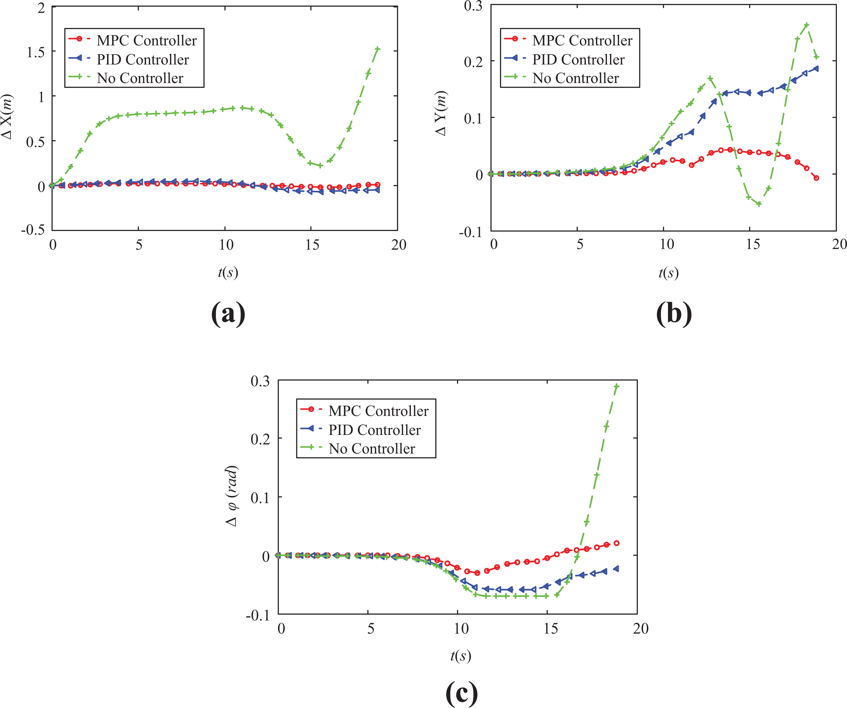
Simulation deviations between actual and reference path. (a) Deviation of X-direction with different control methods. (b) Deviation of Y-direction with different control methods. (c) Deviation of heading angle with different control methods.

The result of parking is considered excellent when the deviation of the heading angle is less than 3°; besides, the deviation of X- and Y-direction are within positive or negative 10 cm when the vehicle is finally stopped. Table 2 lists the deviations between the actual position and the reference position when the vehicle is finally stopped. The deviations of the MPC controller in all directions and the heading angle are minimal, so the parking result is outstanding. The deviations of the PID controller in the X-direction and heading angle are small, while the Y-direction is more significant, therefore the parking result is not satisfactory. The no controller has a significant deviation in all aspects, and it is difficult to meet the requirements of parking.

Table 2.

Parking complete position deviation.

Control algorithm	ΔX end (m)	ΔY end (m)	Δϕ end (rad)
MPC controller	0.0121	−0.0074	0.0207
PID controller	−0.0485	0.1859	−0.0227
No controller	1.5249	0.2066	0.2890

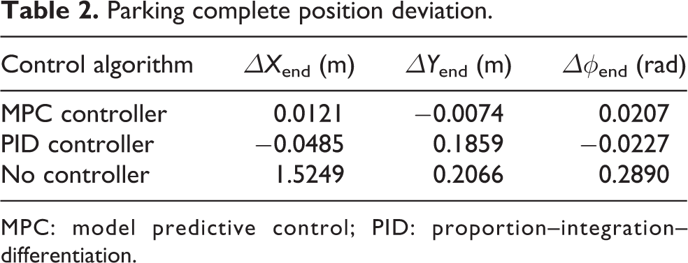
MPC: model predictive control; PID: proportion–integration–differentiation.

Figure 9 is a contrast diagram for different controllers corresponding to the tracking path and the reference path. It can be seen from the diagram that the vehicle can move well along the reference path when the parameters of the MPC controller is reasonable. The final parking position of the vehicle coincides with the reference position. The PID controller is separated from the reference path, and the effect of the parking path tracking is not satisfactory. The tracking effect of the no controller is the worst, and the parking requirement cannot be met.

Figure 9.

Simulation results comparison of path tracking with different control methods.

There are reasons for the different results of the three methods of parking path tracking. Some of the reasons are that the MPC controller directly follows the reference path as the tracking target, considering the deviation of the vehicle’s position and heading angle, speed and front wheel angle, and other reference parameters. Also, the trend of the change in the next period is predicted, and the current control increment is optimized according to the forecast results. Through rolling optimization, the speed of the vehicle and the angle of the front wheel can be coordinated. Therefore, the whole path tracking effect is better. The PID controller is an indirect path tracking control by controlling the speed of the vehicle and the angle of the front wheel. Although the speed of the car can be tracked better, the front wheel angle can be well controlled, however, the two are not organically combined. The factors influencing the accuracy of path tracking considered are simple, and it is blind to pursue the anastomosis of control. It cannot be optimized according to the actual position of the vehicle and the deviation of the position. Therefore, the path tracking result is not satisfactory. The no controller has a significant tracking deviation and no adjustment measures; thus the path tracking result cannot meet the requirements of parking.

Experiment and result analysis

In order to verify the validity and superiority of the proposed MPC algorithm with soft constraints for real vehicle path tracking, the check experiments of path tracking with standard slot whose length is 7 m are carried out. The test prototype is a vehicle which receives control signals to control steering wheel angle, throttle, and brake through controller area network (CAN) bus. The steering wheel angle sensor and the wheel speed sensor are used to collect the steering wheel angle and the vehicle speed, respectively. The inertial navigation device installed on the vehicle is used to collect the real-time position coordinates and heading angles of the vehicle. There are 12 ultrasonic sensors controlled by the parking controller. Eight short-range ultrasonic sensors are installed in front and back of the car body at a certain height which are used to detect obstacles in front or back of the car. Four long-range ultrasonic sensors are installed at the same height on both sides of the car body. The vehicle moves forward along the parking space and the parking slot will be detected by the side ultrasonic sensors. As shown in Figure 10 is the parking controller and inertial navigation device, the parking controller receives the vehicle speed and front wheel angle from the vehicle body CAN bus in real time, meanwhile, it receives the vehicle coordinate and heading angle from the inertial navigation device through serial communication, then calculates the vehicle control variables in the control cycle to control the vehicle.

Figure 10.

Experiment equipment. (a) Parking controller. (b) Inertial navigation device.

The test vehicle and test scenario are shown in Figure 11. The vehicle first stops at the preset position (Figure 11a), then the vehicle starts to reverse along the reference path controlled by the parking controller (Figure 11b), and finally the vehicle stops at the parking slot (Figure 11c). In order to compare the control effects of different algorithms, the parking path tracking experiment based on PID control and no control is carried out, too.

Figure 11.

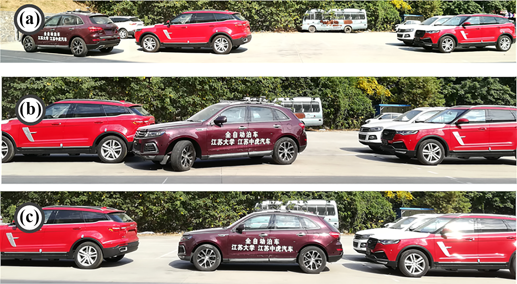
The test scenario of parallel parking. (a) The vehicle stop at the start parking position. (b) Parking process. (c) Parking complete.

The comparison curve between the actual path and the reference path of the real vehicle test is shown in Figure 12. From the diagram, it can be seen that the consistency of the actual path based on MPC controller with the reference path is always high, and the parking effect is fine. There is a larger deviation between the actual path and the reference path based on PID controller. For no control parking path tracking, the actual path significantly deviates from the reference path, therefore, the path tracking effect is poor.

Figure 12.

The experiment results of path tracking with different control methods.

Conclusions

This study is based on the vehicle kinematics model, the linear time-varying path tracking prediction model is derived through a series of transformations such as discretization and Taylor’s formula expansion, which is the basis for the design of the path tracking controller.

The vector relaxation factor is introduced to solve the unfeasible solution problem of the control algorithm. The matrix expression of the predictive optimization problem is derived based on the MPC theory. The linear time-varying model predictive path tracking control is transformed into a linear QP problem with a soft constraint.

The co-simulation is carried out with Simulink/CarSim. The designed controller is used in low-speed parking mode. The simulation results show that the actual path and the reference path are highly consistent in the whole path tracking process, and the final parking result of the vehicle is excellent. The PID control and no control method simulation of path tracking are also carried out in this article. The tracking result is compared with that of the MPC control algorithm. It can be seen that the MPC with softening constraints algorithm is superior to other algorithms in all aspects.

A real vehicle test is carried out for MPC algorithm, and a comparative experiment based on PID control and no control is carried out. The experimental results show that the path tracking effect based on MPC controller is obviously better than that based on PID control and uncontrolled path tracking method.