
Abstract
This article proposes a robust haptics control algorithm for an arm exoskeleton in virtual reality application that guarantees the robustness of the force displaying performance. The developed arm exoskeleton allows the user to sense the profile of virtual objects through joints at wrist, elbow, and shoulder. Forces exerted by the user are directly measured by load cells attached to the links, which are used to determine the corresponding velocity command based on virtual impedance. Due to the imperfection of modeling and the measurement noises from load cells and encoder quantization, the force displaying performance of the device tends to degrade with increasing oscillation, causing permanent damages to the device and user. To solve this problem, a Particle swarm optimization (PSO)-based fixed structure H∞ controller is proposed to control the developed arm exoskeleton. The control performance of the proposed controller is evaluated by both simulation and experiment. The results show that the proposed controller can achieve better tracking performance in comparison with proportional–integral–derivative controller in terms of less oscillation and fast response.
Introduction
With increasing multimedia usage, virtual reality (VR) technology has become more common in daily life, allowing human to interact with virtual environment. A user can see high-quality virtual scene through high-definition screen, hear through surrounding speakers, and interact with virtual environment by using some interacting devices such as keyboards, mouses, or gesture control systems. To fulfill the reality of interaction, force-feedback devices, which can display touch or force-related sensory information from virtual environment to the user, are strongly required. 1
For many years, several force-feedback devices have been released in commercial market for medical surgery training, education, and gaming purposes. Some applications have used VR technology for industrial training to improve workers’ skills in parts assembly, painting and surface finishing. 2 As a result, trainees can practice on virtual parts with no material and model cost. However, one of the key drawbacks of the desktop-type, force-feedback devices available in the market is the limitation to provide only small amount of force which is only suitable for some limited workspaces.
Arm exoskeleton is a structural mechanism that allows users to wear it on their upper limb. It can be used as a force-feedback device for displaying reflection forces at multi-contact points to the user under tele-operation with VR. It can also be used as a power amplifier to manipulate heavy loads. Especially, in haptics applications, the arm exoskeleton can display large reflection forces at shoulder, elbow, and wrist. Workspace for the arm exoskeleton is larger than the desktop type force-feedback device. Furthermore, the arm exoskeleton can be used as either active or passive device.
Even though there have been large numbers of high performance robot arms available in the market, development and control of the arm exoskeleton are still challenging, especially when the large reaction force is required. To achieve the large reaction force, high-performance actuators, appropriate driving mechanisms, and smooth linkages are required. Some of the interesting arm exoskeletons have been developed using different mechanisms and control techniques.
Antonio Frisoli et al. 3 introduced L-Exo which is a tendon driven wearable haptics interface device. In that work, the control of the device was designed based on two impedance controls, acting along tangential and orthogonal directions to the trajectory. The force command was directly converted into the motor torque command using transposed Jacobian method. Tobias Nef et al. developed upper limb exoskeletons in several versions 4,5 for stroke patient rehabilitation. The systems measured the interaction force between human and the robot by a multi-axis force sensor attached at the upper limb. In addition, a force/torque controller with proportional gain was applied as the low-level controller, where its reference force was generated by an impedance controller.
Pierre Letier et al. introduced a 7-degree-of-freedom (DOF) fully portable exoskeleton with a specific kinematics to avoid singularities in the workspace. 6 The device integrated several strain gauges at the joints instead of using multi-axis force/torque sensors. In their work, a technique of friction model compensation using switching mode based on velocity measurement was introduced and implemented in local joint control. The result shows that a hybrid of torque feedback controller can reduce friction in free motion and increase the stability in contact.
Craig Carignan et al. developed a 6-DOF exoskeleton device designed primarily for shoulder rehabilitation and virtual training. 7 The device consisted of three intersection-axis rotary joints mounted on a circular frame surrounding the shoulder. The admittance controller was used to obtain force inputs from the hand.
With regard to the control algorithm point of view, proportional–integral–derivative (PID) controller is widely applied to control forces on the arm exoskeletons to move in the desired position which is generated by either impedance or admittance models. 8 However, the PID controller may not provide the best performance due to the imperfection of modeling, measurement noises, friction, and other disturbance which always degrade performance of the arm exoskeletons. Hence, in this work, PSO-based fixed structure H∞ controller is proposed as the haptics control to solve these problems for the developed arm exoskeleton for VR.
This article is organized as follows. The “Exoskeleton modeling” and “Control architecture” sections describe a dynamic model of the exoskeleton and its control architecture, respectively. The “Controller design” section proposes PSO-based fixed structure H∞ control as the haptics control for the exoskeleton. In the “AIT arm exoskeleton” section, the system architecture of the proposed AIT arm exoskeleton for VR is explained. The “Simulation” and “Experiment” sections provide simulation and experimental results of the control performances of the algorithm, respectively. Finally, the conclusion is made in the “Conclusions” section.
Exoskeleton modeling
Kinematic model
The kinematics configuration of the Asian Institute of Technology (AIT) arm exoskeleton described by Denavit–Hartenberg (D-H) notation is shown in Figure 1. The reference coordinate {0} is assigned at the shoulder joint which is attached to the ground base, and the z-axis of the other reference coordinate is defined along the output shaft of the gearhead of the joint motor. The D-H parameters of the AIT arm exoskeleton are listed in Table 1, where θ is the joint variable, and α, a, and d are the link twist angle, length, and offset, respectively. These parameters are providing in homogenous transformation matrix 9


Coordinate system of the AIT arm exoskeleton.
Denavit–Hartenberg parameters of the AIT arm exoskeleton.

The homogenous transformation matrix that transforms the reference coordinate {6}, which is at the end-effector to the reference coordinate {0}, can be calculated by multiplying individual transformation matrices; that is

Ph
1 and Ph
2 are the positions at which the user’s arm are in contact with the exoskeleton frame at the upper arm and forearm links, respectively. At these positions, three single-axis load cells are installed. The position of reference coordinate {6} is assigned as the haptics interaction point (HIP) and can be directly obtained from the last column of
Dynamic model
The dynamics model of the exoskeleton is derived using Lagrange equation as expressed in equation (3), where
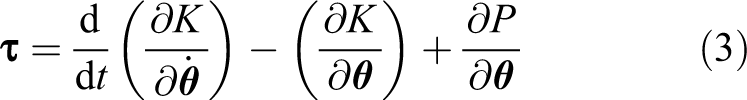
Kinetics and potential energies of the exoskeleton are determined using equations (1), (3), and (5), respectively. We define i as the link index, mi
as the mass of exoskeleton link, irci
∈ R
3×1 as the center of mass (COM) of link i with respect to the ith coordinate, and


The equation of motion is successfully derived in equation (6), where

where
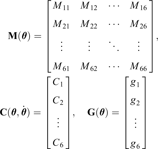
The detail of elements in each terms are given in Appendix 1.
Friction modeling
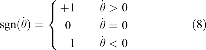
The joint friction is modeled as the combination of both Coulomb and viscosity friction according to Tjahjowidodo et al. 10 and Liu et al. 11 which can be expressed as

Control architecture
In this work, the control architecture of the arm exoskeleton working with VR is illustrated in Figure 2. The human force applying to the device which is sensed by the force sensors is the input of the system. The relationship between input force and the reference position is described by the impedance model. The desired force can be achieved using joint position control.

Control architecture of arm exoskeleton for virtual reality.
Impedance control
An impedance controller is designed to shape the device dynamics to perform the desired behaviors. The desired system dynamics can be described as the relationship between the forces exerting on the virtual object and the result velocities

where

To provide a desired reference point, the system inverse kinematics is applied to determine all joint position command vector
Virtual object dynamics
The force from virtual object in the virtual environment can be modeled according to

where
By taking direct differentiation, the depth rate is determined from
Model compensation
Since the arm exoskeleton system is nonlinear, model linearization is required so that linear controllers can be applied. A computed torque control-based technique is applied in the inner loop to compensate and decouple the nonlinear system, as expressed in equation (12). A block diagram of the feedback linearization is shown in Figure 3. The linear controller is applied in the outer loop for velocity tracking


Feedback linearization block diagram.
Controller design
H∞ robust control
The control block diagram is rearranged into the standard form as shown in Figure 4. The block diagram consists of the generalized plant, P(s), connected with the controller, K(s). P(s) contains the plant together with all weighting functions, while K(s) is the synthesize controller.
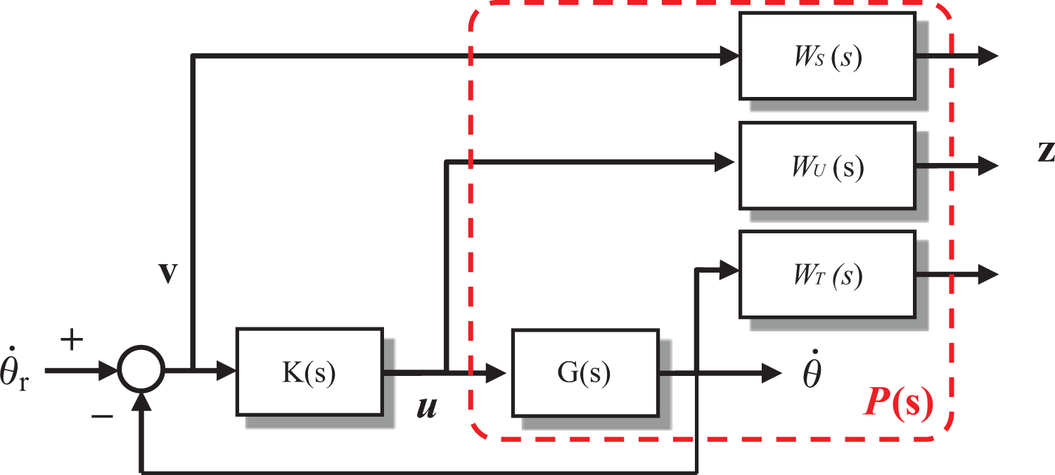
Closed-loop system with performance weights.
The synthesis of H∞ controller consists of finding a state feedback controller K(s) that in any case internally stabilizes the closed-loop system and guarantees that the H∞ norm satisfies the following inequality

S(s) is the sensitivity function which is also the transfer function from the reference signals to the tracking error. T(s) is the complementary sensitivity function and W S(s) is the sensitivity weight, which is desired to have good tracking of reference signal. Thus, the magnitude of W S(s) should be small at low frequencies to reduce the static error, while the filtering cutoff frequency can be interpreted as the minimal system bandwidth. The sensitivity weight, W S(s), is specified as
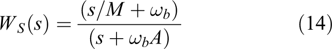
where

where
Robustness is defined by the condition that the closed-loop system is stable for any perturbed system G(s) which can be expressed by

where Gn (s) is the nominal plant and Δ is a stable uncertainty and WT (s) is the complementary sensitivity weight. The direct synthesis of H∞ controller based on solving of a Riccati equation always results in high-order controller which is not appropriate for real implementation. The complexity of the controller synthesis also depends on the selected weight functions. Instead of solving the Riccati equation during the conventional H∞ controller synthesis, a fixed structure H∞ controller alternatively is proposed. PID structure H∞ controller is proposed because of its simple structure. Thus, it is very easy for real implementation but still robust in comparison to the conventional H∞ controller.
However, with the fixed structure H∞ controller, the optimally robust gains cannot be obtained by solving the Riccati equation. Instead, PSO is applied to search for the controller gains that optimize the fitness function which is defined as the system infinity norm.
PSO-based fixed structured H∞ control
A PID controller with a low-pass filter, which has a simple structure, is widely used in several applications. This controller is expressed by
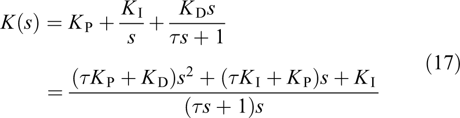
where K P is the proportional gain, K I is the integral gain, K D is the derivative gain, and τ is the time constant of low-pass filter. All parameters are adjusted so that the fitness function in equation (18) is minimum

It is difficult to find the optimal solution if the controller parameters are tuned manually. PSO is a stochastic optimization-based search algorithm based on the simulation of social behavior such as fish schooling and bird flocking. Individual solutions called as particles are “evolved” by cooperation and competition among themselves through generations. Each particle is updated by following two “best” value which is calculated by the fitness or cost function. The particles are manipulated according to the following equations (i denotes the iteration number)


where
AIT arm exoskeleton
Mechanical design
The AIT arm exoskeleton is designed and developed for displaying force feedback rendered by VR at the end-effector which is considered as the HIP with 6-DOFs. The shoulder joint consists of 2-DOF, one with the range of −30°to +90° about the shoulder flexion–extension, and the other with the range of −90° to +30° about the shoulder adduction–abduction. The 1-DOF elbow joint has the range of −90° to 0° about the elbow flexion–extension. Even though the exoskeleton design discards the shoulder medial–lateral rotation due to the complexity of mechanical design, the end-effector of the exoskeleton can move freely along X-, Y- and Z axes in the Cartesian space.
For the 3-DOF wrist joint, a circular link mechanism is designed to surround the user’s forearm with the range of −180° to +90° about the roll direction. The hand holder consists of two intersecting-axis rotary joints with the range of ±30° about the yaw direction and the range of ±45° about the pitch direction.
The exoskeleton frame structure is designed by SolidWorks program (version 2012), which can estimate physical properties of each link such as mass, COM location, and inertia tensor. All these parameters are listed in Table 2.
Physical parameters of the arm exoskeleton.

COM: center of mass.
The real prototype, which is attached to the ground base, is shown Figure 5. The total weight of the device is 21.74 kg. To identify the viscosity coefficient, several fixed currents are applied to the system. The steady-state velocity response and the applied torque, which is proportional to armature current, are then recorded.

Photograph of 6-DOFs AIT arm exoskeleton for virtual reality
At constant speed, the applied torque is equal to the friction torque, 12 which is determined by curve fitting. The identified joint frictions are summarized in Table 3.
Friction coefficients.

System architecture
To provide the rendered force at the end-effector up to a maximum of 100 N, each joint is driven by a DC motor with gearhead. Servo amplifiers are used to drive the motors. The joint angle and its velocity are measured by incremental encoder. Three single-axis load cells are installed to measure the interaction force between the exoskeleton and the user. One load cell is installed at the upper arm bracket and the other two load cells are installed at the forearm bracket. Each load cell has a maximum range of ±100 N. The signal from each load cell is filtered by a second-order low-pass filter with 100-Hz cutoff frequency.
To measure the interaction force between the exoskeleton and the user, the axial forces from three load cells are converted into the interaction joint torques using the following relations
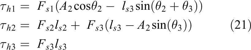
where ls2 and ls3 are the offset distances from the shoulder joint to the upper arm bracket and from the elbow joint to the forearm bracket, respectively.
The main program is run on a PC with PCI interface for data acquisition card (Sensoray 626, Tigard, Oregon, USA) to read the sensing information from all sensors and to send the control signal to the servo amplifiers as shown in Figure 6. The virtual environment and force rendering are developed using Visual C++ with CHAI3D library. This open-source library handles two tasks: graphical rendering task to display the pose of the arm exoskeleton and virtual wall on the screen and force rendering task to detect the collision between the arm exoskeleton and virtual wall to provide the virtual force according to wall stiffness. The force rendering task is executed at the rate of 1000 Hz.

System architecture of the AIT arm exoskeleton.
Simulation
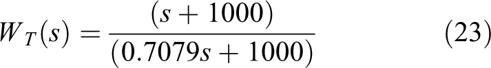
Simulations on the arm exoskeleton are conducted to evaluate the control performances of the proposed PSO-based fixed structure H∞ controller in comparison with the conventional PID controller. To obtain the controller parameters using the proposed control method, firstly the nominal plant model is obtained from the estimated physical parameters. This model is used to determine the fitness function as expressed in equation (18) using MATLAB. In this work, the weight functions, W S(s) and WT (s), are selected as shown in equations (22) and (23), respectively, while Wu (s) is selected as 0.01

The controller parameters are grouped into a position vector p = [K P, K I, K D, τ]T and are searched by the off-line PSO algorithm that minimizes the fitness value. In this work, the inertia w and the learning factors c 1 and c 2 are chosen as 0.9, 0.12, and 1.2, respectively. The optimization terminates if the convergence criteria are satisfied. The cost functions for the first axis, the second axis, and the third axis at each iteration are shown in Figures 7, 8, and 9, respectively.
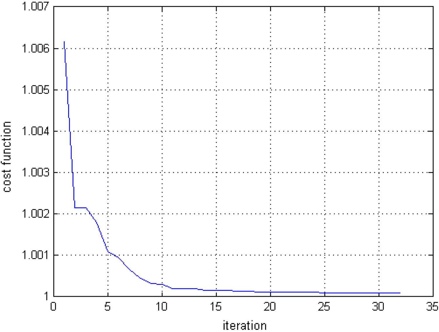
Cost function of each iteration for first axis.

Cost function of each iteration for second axis.

Cost function of each iteration for third axis.
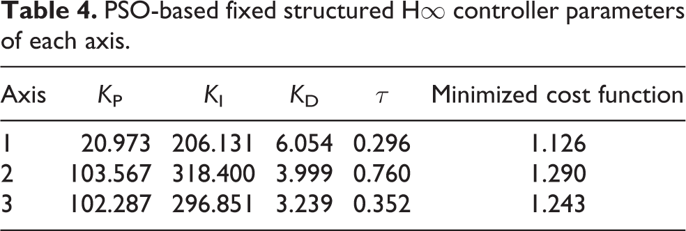
The converged controller parameters of each axis are listed in Table 4.
PSO-based fixed structured H∞ controller parameters of each axis.
The system robustness, time response, and steady-state error are evaluated and compared by simulation on MATLAB Simulink. The external torque is applied to each joint, and finally the reference joint velocity is computed according to the impedance parameters. In the simulation, the impedance parameters are adjusted so that the reference joint velocity has the steady-state value of 1 rad s−1, while the amount of external torque is 1 N·m. Figure 10(a) shows the responses from both the PID controller and the PSO-based fixed structure H∞ controller. The result shows no overshoot and zero steady-state error for the first axis from both controllers.
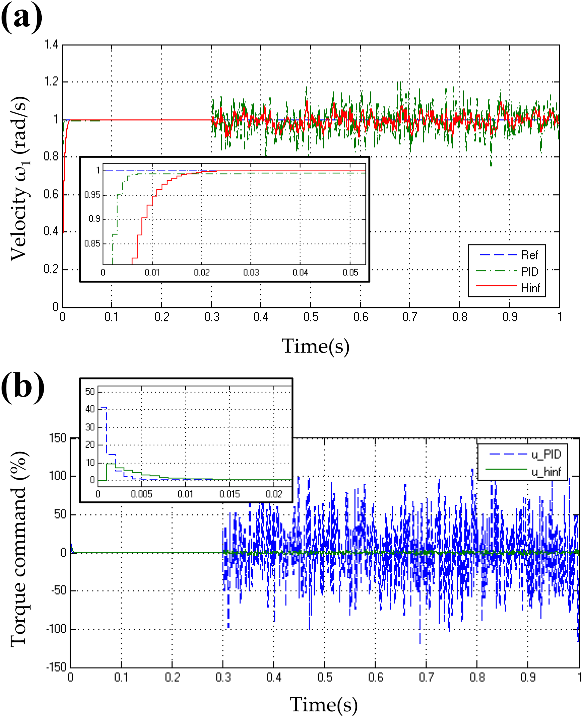
Comparison of (a) velocity step response, (b) control input of first axis under measurement noise (t = 0.3 s).
To investigate perturbation rejection, an external noise of ±1.0 rad s−1 at the frequency of 10 kHz is injected at t = 0.3. The simulation result shows that PSO-based fixed structure H∞ controller can reject the noise from the measured velocity, while the influence of the noise is still seen in the response from PID controller. The control inputs from both controllers are shown in Figure 10(b). The result shows that the control input of PSO-based fixed structure H∞ controller is smoother than that of PID controller.
Figure 11(a) shows that the responses of the second axis from both PID and PSO-based fixed structure H∞ controller have zero steady-state error, no overshoot, and slower responses than the first axis due to larger link inertia. To examine the perturbation rejection in the control input, the external sinusoidal torque 1.0 N·m at 0.5 Hz is injected as the residue of mismatching in model compensation. Both controllers stabilize the closed-loop response; however, the control input generated from PID controller oscillates with high frequency. Similar results are obtained in the responses of the third axis as shown in Figure 12.

Comparison of (a) velocity step response, (b) control input under of the second axis under measurement noise (t = 0.3 s).

Comparison of (a) velocity step response, (b) control input under of the third axis under measurement noise (t = 0.3 s).
Experiment
In the experiments, the proposed controller is implemented on a PC of the AIT arm exoskeleton. Nonlinear term is decoupled as expressed by equation (12), then the outer-loop controller is independently designed to meet the required specification.
To evaluate the robustness and noise rejection performance of the proposed PSO-based fixed structure H∞ controller in comparison with the conventional PID control, three experiments are conducted. In the first experiment, step response analysis is conducted for each axis. The parameters of the conventional PID controller are fine-tuned, so that the step response has no overshoot, zero steady-state error, and the rising time is less than 0.01 s, while the proposed controller is tuned based on robustness criteria. In the second experiment, frequency response analysis is conducted to compare the tracking performance of joint velocity and to investigate the external noise rejection. In the last experiment, the user exerts an external force to the device to freely move and touch the virtual wall.
Both joint torque and joint velocity tracking results are evaluated. All data are collected with the sampling time of 0.01 s.
Step response experiment
The first axis—horizontal shoulder result
Both controllers are tested with joint velocity step command of ±57.1°s−1 (±1.0 rad s−1). As seen in Figure 13(a), there is no overshoot in the response with any steady-state error. The control inputs of two controllers are also observed and compared as shown in Figure 13(b). The result shows that the control input generated by PSO-based fixed structure H∞ controller oscillates with less amplitude than PID controller.

Experimental result of (a) velocity step response, (b) control input of the first axis.
The second axis—vertical shoulder result
The experimental results in Figure 14(a) show no overshoot and no steady-state error in the responses from PID controllers, while the response of the proposed controller has 20% overshoot and slower response. However, there is measurement noise occurred t = 0.4 s, the proposed controller can stabilize. The control inputs from both controllers are shown in Figure 14(b).

Experimental result of (a) velocity step response, (b) control input of the second axis.
The third axis—elbow result
The experimental results in Figure 15(a) show no overshoot and no steady-state error in the responses from both controllers. The control inputs from both controllers are shown in Figure 15(b).

Experimental result of (a) velocity step response, (b) control input of the third axis.
Table 5 summarizes the performance of both controllers for each axis. There are two performance indices: root mean square (RMS) error to indicate tracking performance in velocity command and max(u) to indicate the maximum control input that controller supplies to the actuator.
Comparison of step command tracking performance.

PID: proportional–integral–derivative.
Tracking response experiment
The first axis—horizontal shoulder result
Both controllers are tested with the sinusoidal joint velocity command with amplitude of 60° s−1 and frequency of 0.5 Hz. The result in Figure 16 shows that PID controller is able to control the joint to track sinusoidal command better than PSO-based fixed structure H∞ controller. However, the control input from PSO-based fixed structure H∞ controller has less amplitude than PID controller.

Experimental result of (a) velocity sinusoidal response, (b) control input of the first axis
The second axis—vertical shoulder result
In this experiment, the amplitude of sinusoidal command is changed to 90.0° s−1. The result in Figure 17 shows that PSO-based fixed structure H∞ controller can track the command with no delay, while PID controller has some delay in tracking the command. The disturbance torque from joint friction and imperfect gravity compensation is rejected by PSO-based fixed structure H∞ controller.

Experimental result of (a) velocity sinusoidal response, (b) control input of the second axis.
The third axis—elbow result
The result in Figure 18 shows that H∞ controller of third axis can well reject the disturbance torque from joint friction. The robust controller can track the reference in both high- and low-velocity region, while PID controller is not well under a low speed, which its maximum static error is 28° s−1.

Experimental result of (a) velocity sinusoidal response, (b) control input of the third axis.
Table 6 summarizes the tracking performance to sinusoidal velocity command of both controllers based on the RMS error. From the results, PID controller provides better performance than PSO-based fixed structure H∞ controller for the first axis. However, there is the disturbance torque resulting from imperfect model compensation and measurement noise from encoder quantization as shown in the second and third axes. PSO-based fixed structure H∞ controller can track the low-frequency reference better than PID controller.
Comparison of tracking performance to sinusoidal command.

PID: proportional–integral–derivative; RMS: root mean square.
Force tracking response experiment
This experiment is conducted to validate the force tracking performance of the proposed controller. Firstly, the user exerts torque with small amplitude in both directions (±0.1 N·m) at the elbow joint. After that, the user moves the point toward the virtual wall which is set within the operator range. The interaction torque between the user and the device is measured by a force sensor, while the joint velocity is generated according to the exerted torque.
As the result shown in Figure 19, the velocity in the free motion region shows that PID controller can well track the reference. When contact to the virtual wall, the reference velocity is suddenly changed to zero. The operation mode is changed to force tracking mode. Using PID controller, the overall system has better performance. However, when the velocity noise is generated during the contact, the user feels the vibration which can be measured.
Experimental results of interaction joint torque tracking and joint velocity tracking of convetional PID controller.
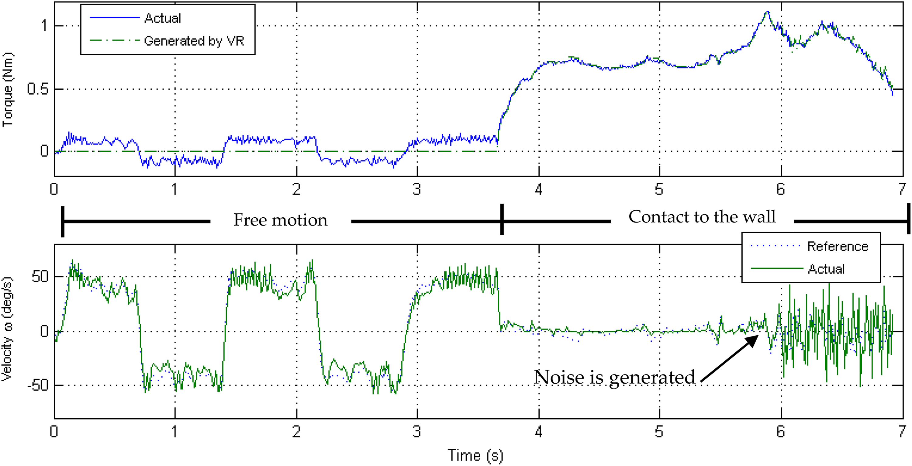
Similarly, Figure 20 shows that PSO-based fixed structure H∞ controller can track both velocity command and joint torque generated by VR. Even though the velocity noise is generated at t = 5.5 s, the proposed controller can efficiently remove the noise that makes the system be stabilized and not effected to the force displaying performance.

Experiment results of interaction joint torque tracking and joint velocity tracking of the proposed controller.
Conclusions
In this research, PSO-based fixed structure H∞ controller was proposed to control the joint velocity of an arm exoskeleton developed at AIT for VR work. Load cells for measuring the interaction between operator and device were used to determine the velocity command using virtual impedance model. The performance of the proposed PSO-based fixed structure H∞ controller is compared with PID controller with model compensation which is one of the popular controllers used in several industry applications.
Both simulation and experimental results show that the proposed controller was able to track the step reference with disturbance torque from imperfect model compensation and noise from encoder quantization. The tracking performance of the proposed controller was better than the conventional PID controller. Moreover, the result showed that the proposed controller provides smoother control command. The interaction torque experiment shows that the proposed controller can stabilize the inner loop, and the performance of force displaying improves.
Footnotes
Declaration of conflicting interests
The author(s) declared no potential conflicts of interest with respect to the research, authorship, and/or publication of this article.
Funding
The author(s) received no financial support for the research, authorship, and/or publication of this article.
Appendix 1
The nonlinear dynamic equation as shown in equation (4). By defining c 1 as cos(θ 1) and s 12 sin(θ 1 + θ 2), there are the details in each element
where
The elements in the Coriolis and centrifugal forces vector, ∈
where cijk is the Christoffel symbol which is calculated by taking partial differentiation of inertia matrix element. 11
The element of gravity vector G(θ) is written as
with the gravity constant
where θi is the joint angle of link i; mi is the mass of link i; Iixx , Iiyy , and Iizz are the moments of inertia of the link frame i; and lci is the length from the center of the link frame to the center of gravity