Sage Journals: Discover world-class research

Abstract

We consider a motion planning problem with task space constraints in a complex environment for redundant manipulators. For this problem, we propose a motion planning algorithm that combines kinematics control with rapidly exploring random sampling methods. Meanwhile, we introduce an optimization structure similar to dynamic programming into the algorithm. The proposed algorithm can generate an asymptotically optimized smooth path in joint space, which continuously satisfies task space constraints and avoids obstacles. We have confirmed that the proposed algorithm is probabilistically complete and asymptotically optimized. Finally, we conduct multiple experiments with path length and tracking error as optimization targets and the planning results reflect the optimization effect of the algorithm.

Keywords

Redundant manipulators task space constraints path planning sampling based asymptotically optimization

Introduction

Task space constrains are common in robotic applications, both in service and in industrial applications. For example, a common task in service applications is to move a water-filled cup with a manipulator. This requires the manipulator to move with a certain posture and a constrained end acceleration. Also for welding occasions, the manipulator needs to follow a given end-effector path which is called welding line. Kinematically redundant robots,¹ such as humanoids or manipulators, possess the dexterity to plan multiple trajectories that meet the task constraints. Therefore, they have the ability to pursue additional objectives, among which the most important is obstacle avoidance. In a complex environment, robot autonomous motion planning requires to plan a trajectory that meets the task space constraints while avoiding self-collision or collisions with environment.

Motion planning in obstacle environment is a very common problem in the field of robotics research. The initial attempts to solve this problem included grid search methods such as the A* algorithm² and artificial potential field methods.³ These algorithms are ideal for mobile robots to perform obstacle avoidance motion planning. For unknown environments with obstacles, Micheal Hoy et al.⁴ reviewed a range of techniques related to navigation of both single and multiple coordinated unmanned vehicles. The main drawback of these methods is their computational complexity and they quickly become computationally intractable with the increase of the configuration space dimension. Wenrui Wang et al.⁵ proposed an improved artificial potential field method for redundant manipulators. However, the calculation of the obstacle potential field is complicated, and the algorithm tends to fall into local extremes for complex environments.

In order to plan a feasible and optimal trajectory, some trajectory optimization methods have been proposed. For example, covariant Hamiltonian optimization for motion planning⁶ optimizes an initial trajectory using covariant gradient descent. For problems with non-differentiable constraints, Mrinal Kalakrishnan et al.⁷ proposed the stochastic trajectory optimization for motion planning method which samples a series of noisy trajectories to explore the space around an initial trajectory. All of the above methods optimize a discrete initial trajectory, and a fine discretization is needed to reason about obstacles in complex environment. Then, the computational cost will increase significantly. To overcome this problem, Gaussian Process Motion Planner⁸ samples a few states on the initial trajectory and uses Gaussian process interpolation to query the trajectory at any time of interest. Trajectory optimization approaches start with an initial trajectory and then optimizes the trajectory by minimizing a cost function. The main disadvantage of these methods is that the optimization effect depends on the choice of the initial trajectory and the solutions are only locally optimal. They are incomplete and not optimal.

Sampling-based approaches have become popular in obstacle avoidance motion planning due to the probability completeness, and they can easily plan a valid path for high degrees of freedom (DOF) systems such as humanoid robots. The most basic sampling-based algorithms are the probabilistic road map (PRM)⁹ and rapidly exploring random trees (RRT).^10,11 Many improved algorithms have also been proposed. For robots with differential constraints, Kuffner and LaValle proposed a control-based RRT algorithm (Kinodynamic RRT),¹² applying robot kinematics to node expansion and finally generating an effective trajectory. In order to obtain the asymptotic optimality, Karaman and Frazzoli¹³ proposed RRT* algorithm, which introduced an optimization structure based on RRT algorithm. Slow convergence is the main disadvantage of this algorithm. To overcome it, Jauwairia Nasir et al.¹⁴ proposed RRT*-SMART algorithm which accelerates the rate of convergence and reduces the execution time effectively. In general, the sampling-based algorithm is very efficient and probabilistically complete. We use this type of algorithm to solve the obstacle avoidance motion planning problem with task constraints for kinematically redundant manipulators.

In this article, we focus on kinematically redundant manipulators and the task is to follow a given end-effector path. Such problems require the robot to follow a path with high precision in continuous time and meet the obstacle avoidance requirements at the same time. Here we use the redundancy of the manipulator to achieve obstacle avoidance, so the planned path will inevitably appear redundant in the joint space. The second goal of this article is to reduce the redundancy of joint trajectories and optimize the trajectory quality. Finally, a high-order smooth joint trajectory facilitates stable operation of the manipulator and it is another goal for this article. The following are the requirements that we have summarized for the planned trajectory:

follow a given path with high precision in continuous time;

avoid self-collision or collisions with environment;

reduce excessive redundancy in joint space; and

meet the requirements of high-order smoothing in joint space.

The remainder of this article is organized as follows. The second section discusses the related work about the task-constrained motion planning problems. In the third section, we formally define the problem and present some expressions and frameworks for the problem. The fourth section describes the entire algorithm in detail. Then, the algorithm is analyzed in the fifth section, including the probability completeness and optimization principle of the algorithm. The sixth section presents the experimental results and illustrates the effectiveness and superiority of the algorithm. Finally, several directions to improve the current work have been mentioned in the concluding section.

Related work

Traditional task-constrained motion is generalized through kinematic control techniques.^15

–18 They are online motion planning that use an inverse of the task Jacobian to track a specified task path. Usually, the internal motions (motions in null-space) that do not perturb the execution of the task will be added for local optimization. So for the problems with obstacles in the environment, some methods^19,20 take the distance from obstacles or the corresponding potential function as an optimization objective to achieve obstacle avoidance. These approaches have proved to be unpractical for realistic motion planning. First, the generation of distance or potential functions is challenging and time-consuming in the high-dimensional joint configuration spaces. Moreover, for manipulators, the problem leads to a nonlinear Two-Point Boundary Value Problem (TPBVP) whose solution can only be solved via numerical techniques. Numerical techniques do not guarantee successful solution and are susceptible to local optimization.

For a more comprehensive exploration of the configuration space, sampling-based algorithms have been proposed such as PRM⁹ and RRT.^10,11 To satisfy the task constraint, Oriolo et al.²¹ proposed a sampling-based algorithm called RRT_LIKE. They divide the joint vector into base joints and redundant joints. Then, they randomly expand the redundant joints and optimize base joints to satisfy the task constraints. The approach was extended to the case of a unified representation of end-effector constraints by Stilman.²² The essence of these planning techniques is to build a road map consisting of admissible configurations. A continuous path will be created by connecting these admissible configurations (typically, a linear connection). Hence, the path between two admissible configurations cannot strictly meet the task constraints. For path tracking issues, a higher sampling rate in the task space can reduce tracking error, but the calculation time will increase. The main disadvantage of such algorithms is that they cannot meet the task constraints in continuous time and have low tracking accuracy for the problems with a given end-effector path.

To solve this problem, Oriolo and Vendittelli²³ apply kinematic control techniques to sampling-based algorithms. They divide the specified task path into multiple leaf areas. Then, they use the reverse kinematics of redundant manipulators to track the given path, and a random self-motion in null space is utilized to realize random expansion. This approach was extended to the repetitive task constraints problems (e.g. repeatedly tracking an elliptical track) by Cefalo et al.²⁴ and Oriolo et al.²⁵ The approach essentially uses the self-motion in null space to achieve obstacle avoidance, and the planned path will inevitably be redundant in joint space. So the path generated by it can only satisfy constraints, but not optimal.

To achieve asymptotic optimization, we propose an optimized algorithm builds upon Oriolo and Vendittelli.²³ The core task of the algorithm is to let the manipulator follow the given end-effector path with high precision. Meanwhile, the proposed algorithm introduces an optimization structure in the joint path generation process. Currently, the tracking accuracy in task space and the path length in joint space are optimized. We have confirmed the probability completeness of the algorithm and have illustrated the optimization principle of the algorithm. The salient features of the proposed algorithm are as follows.

Complete probability: The proposed algorithm is sampling-based and we have proved this property in the fifth section.

High tracking accuracy: We use the reduced gradient method^26,27 and the error feedback mechanism for nodes connection to ensure the end-effector path tracking accuracy in continuous time.

Low joint path redundancy: Sampling-based approach can easily lead to redundancy for the planned path in joint space. The proposed algorithm introduces an optimization structure in the path generation process and shortens the length of the planned path in joint space significantly.

High-order smoothing for the planned joint trajectory: As mentioned before, we use the reduced gradient method for node connections and this allows us to perform a fifth-order polynomial programming on redundant joints.

Preliminary material

The proposed optimized algorithm in this article is improved on the basis of the algorithm given by Oriolo and Vendittelli.²³ So we will adopt the expression and framework introduced in it. Meanwhile, since the article mainly focuses on kinematically redundant manipulators, we assume that the robot is not subject to nonholonomic constraints.²⁸

Kinematics model

Consider a robot with configuration q and its n_q -dimensional configuration space is denoted by C. Let C_obs be the set of obstacles in the configuration space. Correspondingly, C\C_obs will be the obstacle-free space which is called C_free . The movement of each joint can be seen as a process of continuous integration. The admissible tangent vectors to a configuration space path q(s) can be used as an integral object, where $s \in [0, 1]$ is a path parameter and the tangent vectors can be denoted as

q^{'} = \frac{d q}{d s} = \tilde{ν}

where $\tilde{ν}$ represents geometric inputs. When s is the time, $\tilde{ν}$ represents velocity inputs and a trajectory will be generated directly rather than a path. The manipulator is naturally described and controlled in joint space, while its operation is usually specified in task space.¹⁷ We use vector t to indicate the location of the manipulator end effector in task space. The relationship between t coordinates and q coordinates is expressed by the forward kinematics equation

t = f (q)

where f is a nonlinear forward kinematics function. The differential form is

t^{'} = J (q) q^{'} = J (q) \tilde{ν}

where $J (q) = \partial f / \partial q$ is the n_t × n_q task Jacobian matrix which maps the available geometric inputs to the admissible task space tangent vectors. For a serial-chain manipulator, when n_q > n_t , we consider the robot is kinematically redundant. For a specific task vector t, the corresponding joint vector q will not be unique and even an (n_q – n_t )-dimensional subset of C.

Problem formulation

Consider a specific path t_d (s) in task space with $s \in [0, 1]$ , and the path is differentiable. The task-constrained optimized motion planning problem is to find a path q(s) in configuration space, $s \in [0, 1]$ , such that

$t_{d} (s) = f (q (s)), \forall s \in [0, 1]$ ;

the robot does not collide with obstacles or with itself throughout the path; and

the generated configuration space path is asymptotically optimized with continuous iteration.

Due to task constraints, the planning space for this problem is

C_{t a s k} = {q \in C : f (q) = t_{d} (s), s \in [0, 1]}

For each $s \in [0, 1]$ , there will be a sub-planning space which is called leaf as mentioned by Oriolo and Vendittelli.²³ A generic leaf is defined as

L (s) = {q \in C : f (q) = t_{d} (s)}

and

C_{t a s k} = \underset{s \in [0, 1]}{\cup} L (s)

So the manifold C_task has a foliation structure naturally which consists of multiple leaf regions. The process of motion planning is to connect each leaf in the intersecting space $C_{t a s k} \cap C_{f r e e}$ . Meanwhile, the asymptotic optimization can be achieved by optimizing the connection between adjacent leaves.

Motion generation

In this article, motion generation is divided into two types, that is, forward motion generation and steering motion generation. The forward motion generation is to generate an arbitrary configuration belongs to the next leaf from a given initial configuration. Differently for the steering motion generation, the initial configuration and the goal configuration are specified and the task is to generate a valid smooth path in joint space.

Forward motion generation

The purpose of forward motion generation is to satisfy the probability completeness of the algorithm, and it steers the robot to an arbitrary configuration that belongs to the next leaf. The planning process is generated by the following scheme

q^{'} = J_{t}^{†} (q) ({t^{'}}_{d} + k e_{t}) + (I - J_{t}^{†} (q) J_{t} (q)) ω

where $J_{t}^{†} (q)$ is the pseudoinverse of task Jacobian J_t (q), e_t = t_d − t is the task error, k is an error gain, $(I - J_{t}^{†} (q) J_{t} (q)) ω$ is called self-motion which belongs to the null space of the task Jacobian, and ω is an arbitrary n_q -dimensional vector that acts as a residual input. The motion generation between adjacent leaves is done by a simple Euler method with an integration step Δs. So equation (4) can be discretized as follows

\begin{matrix} \frac{q_{n + 1} - q_{n}}{Δ s} = J_{t}^{†} (n) (\frac{t_{d} (n + 1) - t_{d} (n)}{Δ s} + k (t_{d} (n) - t (n))) \\ + (I - J_{t}^{†} (n) J_{t} (n)) ω (n) \end{matrix}

Then, we set the error gain k to be 1/Δs and equation (5) will be converted as follows

\begin{matrix} q_{n + 1} - q_{n} = J_{t}^{†} (n) (t_{d} (n + 1) - t (n)) \\ + α (I - J_{t}^{†} (n) J_{t} (n)) ω (n) \end{matrix}

where α denotes self-motion coefficient, and t(n) and t_d (n + 1) represent the current actual pose and the desired pose of the next moment in the task space, respectively.

Considering that if a damping coefficient²⁹ is introduced to solve the problem of singular configurations, it will reduce the tracking accuracy. So in this article, we set $J_{t}^{†} = J_{t}^{T} {(J_{t} J_{t}^{T})}^{- 1}$ and discard all singular configurations.

For the purpose of ensuring the tracking accuracy of the system, the norms of the two terms in the right-hand side (rhs) of equation (6) are constrained in a certain proportion β by adjusting the self-motion coefficient α. The larger the α, the faster the exploration of feasible space is. However, as the value of α increases, the total path length and the tracking error will increase. So a suitable limit proportion is necessary.

In order to achieve the randomness of exploring, each value in the residual input vector ω is randomly generated. Meanwhile, this process is simply to generate a valid configuration that belongs to the next leaf, and the path will be optimized in the following process, so the residual input vector ω is constant throughout the integration interval [s_k , s_k _{+ 1}] and does not need to consider path smoothing.

Steering motion generation

The purpose of steering motion generation is to optimize the connections of existing nodes in the tree as is shown in the next section. So the initial configuration and the goal configuration are specified. There are two requirements need to be met for this motion. The first is the task constraint, and the second is to meet the constraint of the goal configuration. Here, we adopt the reduced gradient method introduced by Luca et al.²⁶ and make some improvements to smooth the joint path.

For an m-dimensional task constraints, the core of the algorithm is to divide the n-dimensional configuration space of redundant manipulators into two parts: q_r and q_b , where the redundant coordinates q_r is (n − m)-dimensional, and the base coordinates q_b is m-dimensional. Then plan the redundant coordinates q_r to move the manipulator to the specified goal configuration and adjust the base coordinates q_b to satisfy the task constraint.

Correspondingly, the m × n task Jacobian J_t (q) in equation (4) can be block partitioned as J_t = (J_t _,r J_t _,b), where J_t _{, r} is m × (n − m) and J_t _{, b} is m × m. The number of possible ways for the division is $C_{n}^{m}$ and $C_{n}^{m} = n! / m! (n - m)!$ The selection criterion for m-dimensional base coordinates is to ensure that matrix J_t _{, b} is non-singular.

At a differential level, the direct kinematic relation can be written as

t^{'} = J_{t} q^{'} = [\begin{matrix} J_{t, r} & J_{t, b} \end{matrix}] [\begin{array}{l} {q^{'}}_{r} \\ {q^{'}}_{b} \end{array}] = J_{t, r} {q^{'}}_{r} + J_{t, b} {q^{'}}_{b}

In order to improve the tracking accuracy, we introduce a negative feedback mechanism

{e^{'}}_{t} = {t^{'}}_{d} - t^{'} = - k e_{t}

where e_t = t_d − t. Considering that the matrix J_t _{, b} is non-singular, equation (7) can be converted to

J_{t, b}^{- 1} ({t^{'}}_{d} + k e_{t}) = J_{t, b}^{- 1} J_{t, r} {q^{'}}_{r} + {q^{'}}_{b}

Then

{q^{'}}_{b} = - J_{t, b}^{- 1} J_{t, r} {q^{'}}_{r} + J_{t, b}^{- 1} ({t^{'}}_{d} + k e_{t})

From equation (10), it can be seen that the base coordinates q_b are determined by the task constraints and the redundant coordinates q_r . By the above negative feedback mechanism, the task coordinates t will converge exponentially to the final desired value t_d _{, k+1}. So in the case of the matrix J_t _{, b} non-singular, the calculated base coordinates q_b can ensure that the task constraints are met regardless of the choice of q_r .

Then, we plan the redundant coordinates q_r to meet the constraints of the goal configuration. Given a pair of configurations (q_k , q_k ₊₁) to be joined, where q_k belongs to the leaf L_k and q_k ₊₁ belongs to the leaf L_k ₊₁. The configurations q_k and q_k ₊₁ are the nodes already in the random tree, so the boundary geometric velocities and accelerations are specified. Corresponding to redundant coordinates, the task is to make a connection between $(q_{r, k}, {q^{'}}_{r, k}, {q^{″}}_{r, k})$ and $(q_{r, k + 1}, {q^{'}}_{r, k + 1}, {q^{″}}_{r, k + 1})$ . Note that in the actual experiment, we set the accelerations of each configuration on leaves to 0. The same as the forward motion generation, we set the integration step size Δs between s_k and s_k ₊₁. To smooth the subpath and keep the continuity of accelerations, we adopt a fifth-order polynomial to plan each component of vector q_r , respectively, as follows

\begin{matrix} q_{i, r} (s) = a_{i 5} {(s - s_{k})}^{5} + a_{i 4} {(s - s_{k})}^{4} + a_{i 3} {(s - s_{k})}^{3} \\ + a_{i 2} {(s - s_{k})}^{2} + a_{i 1} (s - s_{k}) + a_{i 0} \end{matrix}

where $s \in [s_{k}, s_{k + 1}]$ , and q_i _{, r}(s) denotes the ith component of vector q_r . The scalars a_i ₀, a_i ₁, a_i ₂, a_i ₃, a_i ₄, and a_i ₅ can be computed by the following boundary conditions

\begin{array}{l} q_{i, r} (s_{k}) = q_{i, r, k}, q_{i, r} (s_{k + 1}) = q_{i, r, k + 1} \\ {q^{'}}_{i, r} (s_{k}) = {q^{'}}_{i, r, k}, {q^{'}}_{i, r} (s_{k + 1}) = {q^{'}}_{i, r, k + 1} \\ {q^{'}}^{'}_{i, r} (s_{k}) = {q^{'}}^{'}_{i, r, k}, {q^{'}}^{'}_{i, r} (s_{k + 1}) = {q^{'}}^{'}_{i, r, k + 1} \end{array}

Then, the geometric inputs ${q^{'}}_{r}$ between s_k and s_k ₊₁ can be easily computed. From equation (10), we can see that the smooth task track t_d (by assumption) and the smooth redundant coordinates q_r can ensure that q_b is smooth.

As mentioned before, the task coordinates t converge to the desired task value t_d _{, k+1}. Meanwhile q_r converges to q_r _{, k+1}, therefore q_b is destined to converge to one of the inverse kinematic solutions of the degenerate robot corresponding to the desired task value t_d _{, k+1}. Here, the degenerate robot is a redundant manipulator whose redundant coordinates q_r frozen at q_r _{, k+1}. When the degenerate robot is noncuspidal³⁰ and q_b _{, k} and q_b _{, k+1} belong to the same homotopy class (which was defined by Oriolo et al.²⁵), q_b _{, k} will converge to q_b _{, k+1} and the detailed proofs have been given by Oriolo et al.²⁵

For this method, there are some points that need attention in practice. The first is that the preconditions it needs are not always satisfied, so we will discard the optimized connection when q_b _{, k} cannot converge to q_b _{, k+1}. Second, when the specified path has speed constraints, the computed $q^{'}$ will be actual velocity inputs rather than geometric inputs, so the velocity and acceleration constraints of each joint need to be considered.

In fact, using the process 2 of steering motion generation, the randomness of the algorithm can also be achieved by randomly generating redundant coordinates q_r . However, we still use the process 1 of forward motion generation for several reasons. First, it takes very little extra time to generate a random configuration. Next, using the configuration generated by process 1 can establish effective connections between two adjacent leaves with greater probability. Finally, the parameter β can well control the exploratory nature of the tree and is useful in a complex environment.

Tree extension

Our randomized planner introduces the idea of optimal RRTs (RRT*s)¹³ and builds an asymptotically optimized rapidly exploring random tree in task-constrained configuration space C_task , as shown in Figure 1. The whole algorithm is given in Algorithms 1 to 3. Before building the trees, we use an equispaced sequence of N + 1 path parameter values ${s_{0} = 0, s_{1}, \dots, s_{N - 1}, s_{N} = 1}$ to sample the desired task path t_d (s). Then, each path parameter value has an associated leaf index i (i = 0,…, N) which identifies the particular leaf L(s_i ). Correspondingly, we use the shorthand notations t_d _{, i} = t_d (s_i ) and L_i = L(s_i ).

Figure 1.

The extension of an asymptotically optimized rapidly exploring random tree. The dotted lines in the figure indicate the original connections and the solid lines indicate the optimized connections.

Algorithm 1.

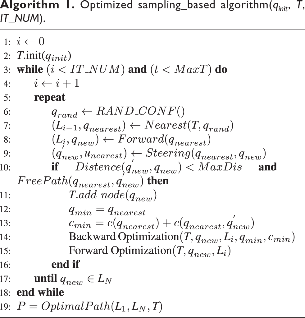
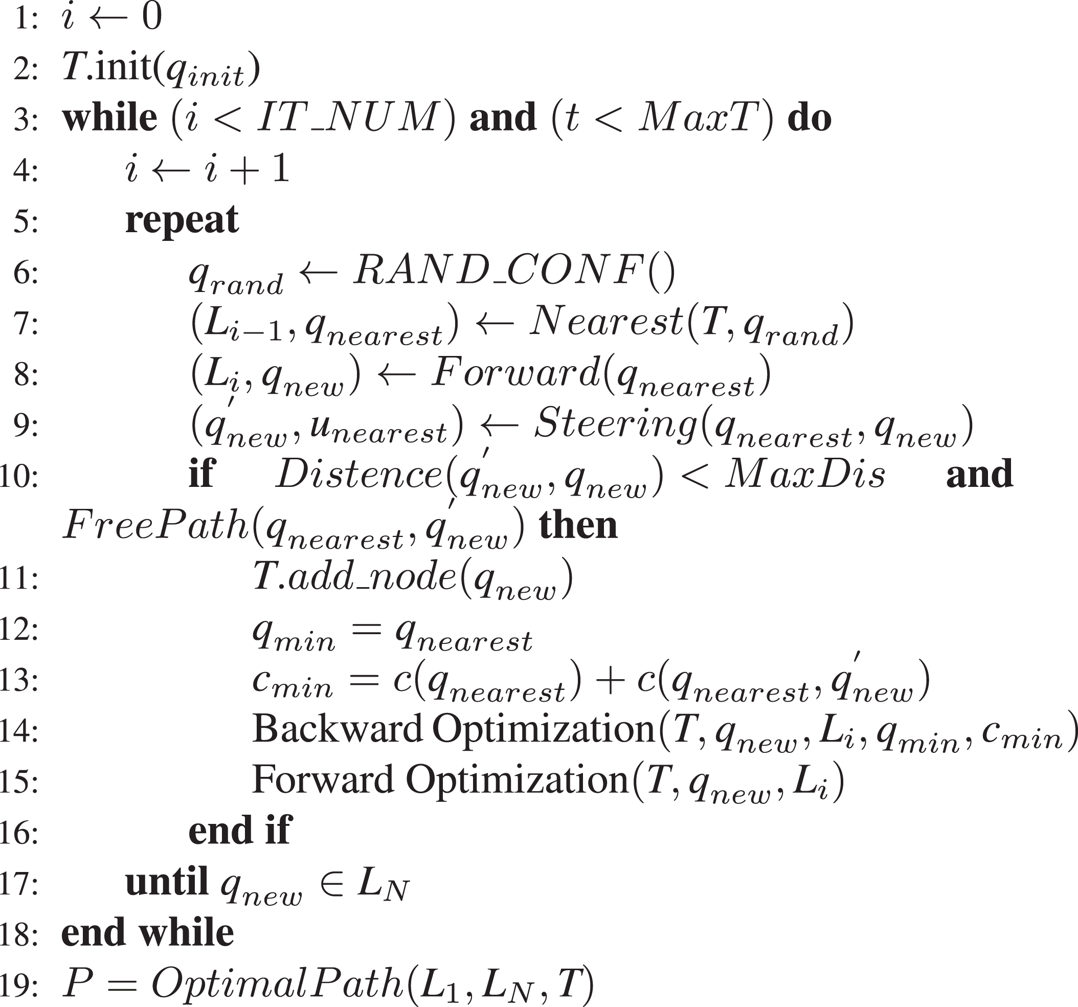
Optimized sampling_based algorithm( $q_{i n i t}$ , T, IT_NUM).

Algorithm 2.

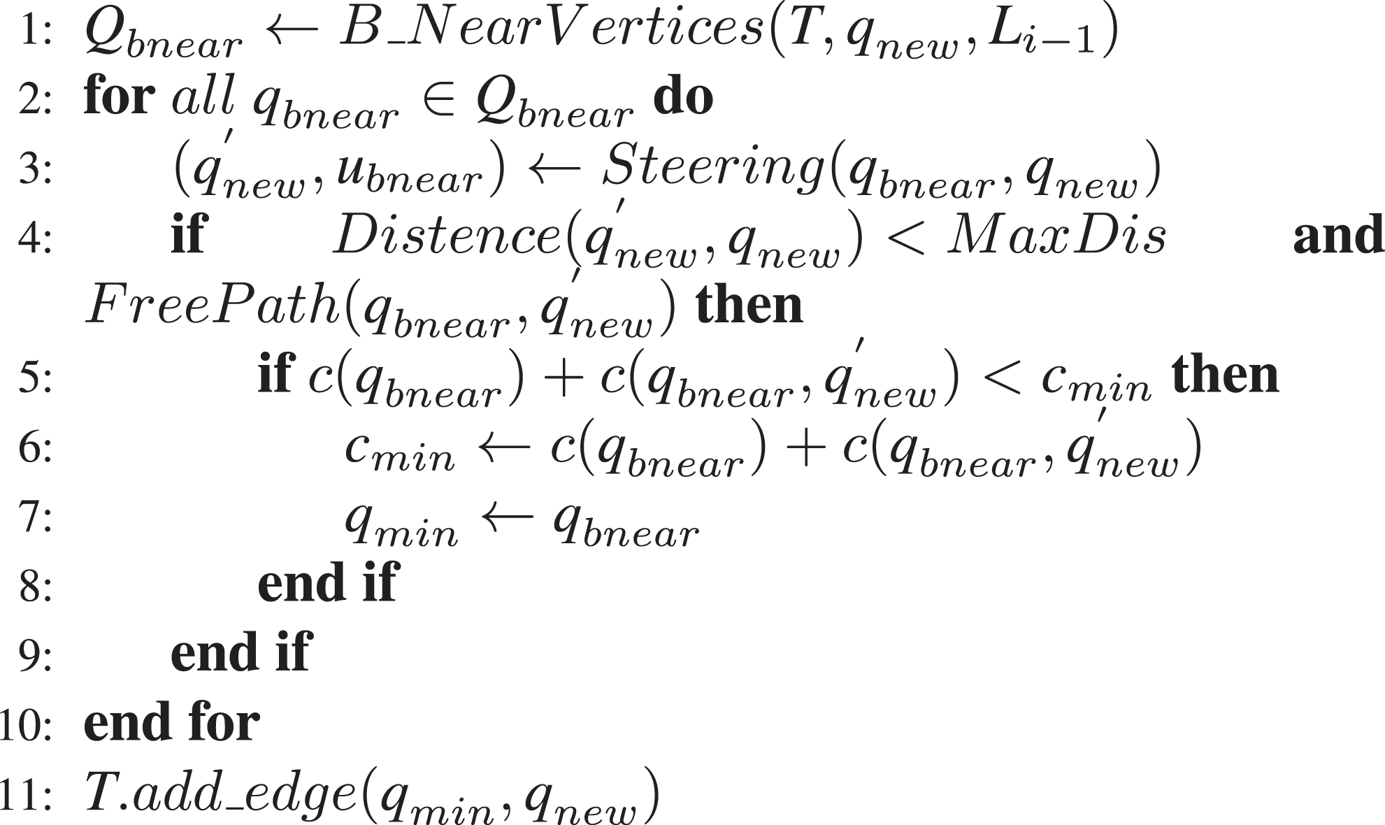
Backward optimization(T, q $_{n e w}$ , $L_{i}$ , q $_{min}$ , c $_{min}$ ).

Algorithm 3.

Forward optimization(T, $q_{n e w}$ , $L_{i}$ ).

The main procedure of tree extension is shown in Algorithm 1. First, a given initial state $q_{i n i t}$ lies in L ₀ and a random configuration $q_{r a n d}$ in C is generated by RAND_CONF. Then, the algorithm searches the nearest configuration $q_{n e a r e s t}$ in the tree T and the corresponding leaf index is i − 1 (line 7). Next, use the Forward procedure which is called forward motion generation before to generate a new configuration $q_{n e w}$ in the next leaf L_i . Then, the Steering procedure which is called steering motion generation before will be used to create a smooth path between $q_{n e a r e s t}$ and $q_{n e w}$ . As is mentioned in the last section, q_b does not always converge to q_b _{, k+1}, so a new configuration ${q^{'}}_{n e w}$ is generated. Only when the Euclidean distance between ${q^{'}}_{n e w}$ and $q_{n e w}$ is within the maximum allowable distance MaxDis, we can conclude that $q_{n e a r}$ can be steered to $q_{n e w}$ . When $q_{n e a r}$ can be steered to $q_{n e w}$ and the smoothing path between $q_{n e a r e s t}$ and $q_{n e w}$ is collision free, $q_{n e w}$ will be added to the tree (lines 10–13) and the following is the optimization process. When the new configuration $q_{n e w}$ belongs to the end leaf L_N , a valid path is generated. In our planner, the algorithm will stop when the specified number of valid path IT_NUM is reached or the algorithm runs longer than the specified time. Finally, choose the optimal path among multiple valid paths (line 19).

The optimization process which is shown in Algorithms 2 and 3 is the core of the planner. Different from the traditional RRT* algorithm,¹³ in our planner, we divide the optimization process into two parts: backward optimization and forward optimization. The backward optimization is to select an optimal parent node of $q_{n e w}$ as follows. First, the B_NearVertices procedure is invoked to determine the set $Q_{b n e a r}$ which consists of configurations near $q_{n e w}$ on the leaf L_i ₋₁ (line 1). Then use the Steering procedure to generate a path from $q_{b n e a r}$ to $q_{n e w}$ that follows the task constraints. As mentioned before, a new configuration ${q^{'}}_{n e w}$ will be generated. Only when the Euclidean distance of ${q^{'}}_{n e w}$ and $q_{n e w}$ is within the maximum allowable distance MaxDis, we can conclude that the $q_{b n e a r}$ can be steered to $q_{n e w}$ . So among the configurations in $Q_{b n e a r}$ , the configuration that can be steered to $q_{n e w}$ and incur minimum cost is chosen as the parent node (lines 2–11).

After $q_{n e w}$ is connected to the tree T, the forward optimization procedure attempts to connect $q_{n e w}$ to configurations that are already on the leaf L_i ₊₁. First, similar to the previous, the F_NearVertices procedure is to determine the set $Q_{f n e a r}$ in the leaf L_i ₊₁ (line 1). Then for any configurations $q_{f n e a r}$ in $Q_{f n e a r}$ , if the Steering procedure can generate a collision-free path between $q_{n e w}$ and $q_{f n e a r}$ and the cost it incurs less than the current cost of $q_{f n e a r}$ , $q_{n e w}$ will be the new parent node of $q_{f n e a r}$ and the configuration $q_{f n e a r}$ is optimized. The optimization process updates the cost of $q_{f n e a r}$ , so we need to treat $q_{f n e a r}$ as a new configuration and perform a forward optimization for it. Then, the self-invocation will produce an inner loop until the next leaf has no nodes or optimized to the end leaf L_N (lines 10–12). Note that in actual programming, in order to avoid double counting, we create a table to record the cost of each valid connection.

Algorithm analysis

In this section, we will confirm the probability completeness of the algorithm and illustrate the optimization principle of the algorithm.

Probabilistic completeness

We will now confirm the probability completeness of the planner. Explain in advance that this proof draws on some of the claims given by Oriolo et al.²⁵ The optimization procedure is simply to optimize the connection without reducing the connection between adjacent leaves, so it does not affect the convergence properties of the algorithm. Then for the sake of proof, we now simplify the planner by only using the process of steering motion generation to smooth the path generated by forward motion generation without any optimization.

Assume that there is a valid path q*(s) which is generated by the simplified planner. Then our purpose is to confirm that the probability which the simplified planner can generate such path converges to 1, with constant iteration.

The configuration of the path q*(s) on each leaf L_i is generated by forward motion generation. Meanwhile, the subpath between any two adjacent leaves L_i and L_i ₊₁ is generated by steering motion generation and the function is continuous in equations (10) and (11). So two spherical neighborhoods exist, S(q*(s_i )) for q*(s_i ) and S(q*(s_i _{+ 1})) for q*(s_i ₊₁), where q*(s_i ) and q*(s_i ₊₁) belong to L_i and L_i ₊₁, respectively. For any pair of configurations (q ₁, q ₂) with $q_{1} \in S (q^{*} (s_{i}))$ and $q_{2} \in S (q^{*} (s_{i + 1}))$ , q ₁ can be steered to q ₂ by the process of steering motion generation.

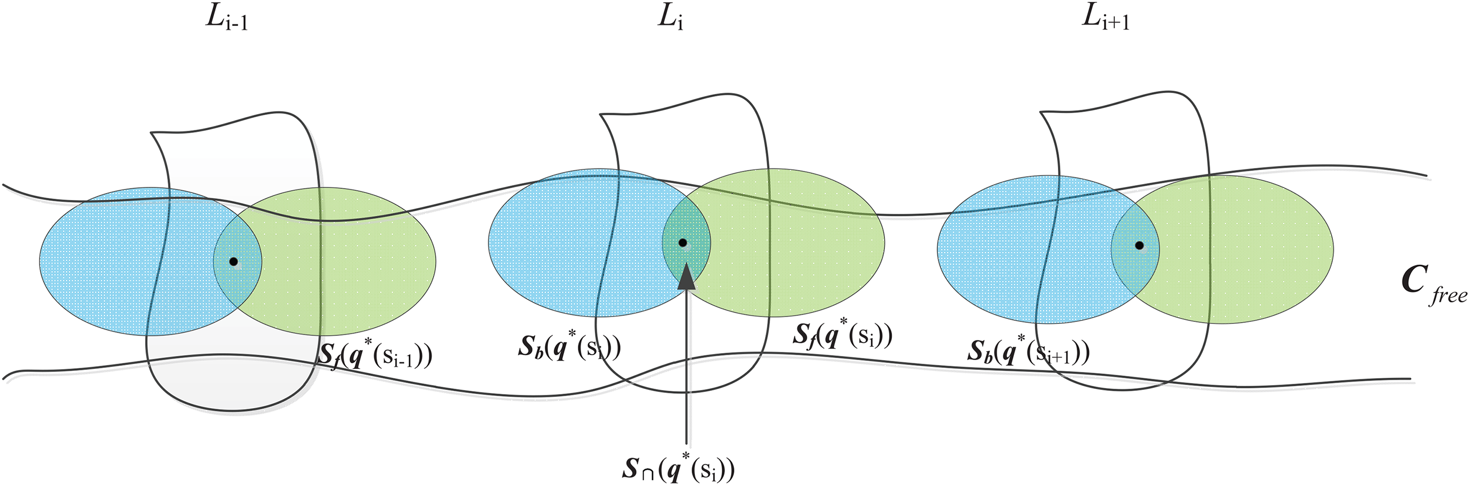
For any intermediate configuration q*(s_i ) in the path, it has two spherical area S_b (q*(s_i )) and S_f (q*(s_i )) corresponding to the front and back configurations as shown in Figure 2. Note that q*(s_i ) belongs to the intersection of S_b (q*(s_i )), S_f (q*(s_i )), C_free , and L_i , so the intersection is not empty and we set $S_{\cap} (q^{*} (s_{i})) = S_{b} (q^{*} (s_{i})) \cap S_{f} (q^{*} (s_{i})) \cap C_{free} \cap L_{i}$ . Then, the problem can be converted to prove that the configurations in $S_{\cap} (q^{*} (s_{i}))$ can be generated by forward motion generation.

Figure 2.

The schematic diagram of intersection area for adjacent configurations.

The valid subpath to q*(s_i ) can be denoted as follows

Q_{i}^{*} (s) = {q^{*} (s_{k}), k \in [s_{0}, s_{i}]}

where the coefficient i can begin from 1 to N. Since the configurations in $Q_{i}^{*} (s)$ are generated by forward motion generation, each of them corresponds to a residual input $ω_{k}^{*}$ and the collection of them is denoted as

W_{i}^{*} = {ω_{0}^{*}, ω_{1}^{*}, \dots, ω_{i}^{*}}

Combined with equation (4), we can see that the special area $S_{\cap} (q^{*} (s_{i}))$ corresponds to an area $S (ω_{i}^{*})$ , and each configuration q_i in $S_{\cap} (q^{*} (s_{i}))$ can be integrated by equation (4) with a corresponding residual input ω_i in $S (ω_{i}^{*})$ .

Then the problem can be converted to produce a series of residual inputs $ω_{0}, ω_{1} \dots ω_{i}$ which belong to $S (ω_{0}^{*}), S (ω_{1}^{*}) \dots S (ω_{i}^{*})$ , respectively. Considering that the measure of $S (ω_{i}^{*})$ is nonzero and the residual inputs $ω_{0}, ω_{1} \dots ω_{i}$ are randomly generated, the probability to produce a series of residual inputs that meet the above requirements tends to 1 as the number of iterations increases. In combination with the above analysis, the probability completeness of the planner has been proved.

Algorithm optimization

In our approach, we divide the optimization process into two parts: backward optimization and forward optimization. The core theory is similar to the idea of dynamic programming.³¹ For two configurations (q ₁, q ₂) on the adjacent leaves (L_i , L_i ₊₁), if the cost of connecting from the initial configuration $q_{i n i t}$ to q ₂ via q ₁ is the lowest compared to all other configurations on the leaf L_i , we call q ₁ the optimal parent node of q ₂.

In our planner, when a new configuration $q_{n e w}$ is introduced into the tree T, we will carry out two processes of forward optimization and backward optimization.

In the backward optimization process, we search the optimal parent node of $q_{n e w}$ as shown below

q_{p a r e n t} = \underset{q \in Q_{b n e a r}}{arg min} (c (q) + c (q, q_{n e w}))

To reduce calculation consumption, we just search in area $Q_{b n e a r}$ instead of the entire area of leaf L_i ₊₁ and discard the configurations away from $q_{n e w}$ on leaf L_i ₋₁. From this process, we can insure that $q_{n e w}$ is connected to its optimal parent node and the path from $q_{i n i t}$ to $q_{n e w}$ is optimal under the current situation.

Then, the forward optimization is to determine whether $q_{n e w}$ is the optimal parent node of configurations $q_{n e a r}$ on the next leaf L_i ₊₁ and the true will be updated. As the optimization process updates the cost of $q_{n e a r}$ , it will affect the judgment of the configurations on the next leaf for their optimal parent nodes. So we perform the process of forward optimization on the updated node $q_{n e a r}$ . Then, the self-invocation will produce an inner loop and the process ensures that the configurations on all subsequent leaves are still connected to their optimal parent nodes.

The optimization process can be converted to a typical dynamic programming model as shown in Figure 3. Each leaf corresponds to a stage and each configuration corresponds to a state. Then, the forward state transition equation is

cost (q_{m, i}) = m in {c (q_{i - 1 :}) + c (q_{i - 1 :}, q_{m, i})}

Figure 3.

The schematic diagram of dynamic programming.

where q_i _–1: represents all states in the stage i − 1. It is similar to equation (15).

In our approach, each configuration in the tree T is connected to its optimal parent node through the above optimization process. So each connection in the tree T satisfies equation (16) and the generated path is optimal under the existing situation.

As new nodes are added, the resulting path will be optimized continuously. However, the subpath is generated by equations (10) and (11) and it is not optimal subpath. So the resulting path is asymptotically optimized, but not asymptotically optimal.

Simulation results

We have implemented our algorithm in C++ and rely on an open source motion planning platform MoveIt!³² which has been released into the Robot Operating System (ROS). All simulations run on a personal computer with 3.7 GHz Intel CPU and 8 GB memory under a 64-bit Ubuntu operating system.

We perform simulation experiments on a traditional 6-DOF robot and a 7-DOF KUKA LWR manipulator, respectively. In all experiments, we set the optimization goal or the cost of configurations as

c (q) = L (q) + λ e (q)

where L(q) is the path length from q _init to q in the configuration space C, e(q) is the average tracking error, and λ is the weight of the tracking error.

We get the path length L(q) by superimposing each integration segment and the distance for n_q -DOF joint robot in C is computed by

d (q_{1}, q_{2}) = \sum_{i = 1}^{n_{q}} min {| θ_{i,1} - θ_{i,2} |, 2 π - | θ_{i,1} - θ_{i,2} |}

The tracking error is obtained by accumulating the error of each integration point in the task space and then calculating the average. For each integration point, its tracking error is computed by

e_{t} = {[{(t_{x} - t_{d x})}^{2} + {(t_{y} - t_{d y})}^{2} + {(t_{z} - t_{d z})}^{2}]}^{1 / 2}

We will present numerical experimental results and illustrate the performance of the optimized planner compared to the algorithm without optimization proposed by Oriolo and Vendittelli.²³ In order to ensure the fairness of the comparative experiment, we avoid self-motions $({t^{'}}_{d} = 0)$ which is mentioned by Oriolo and Vendittelli.²³

A KUKA LWR manipulator drawing an arc

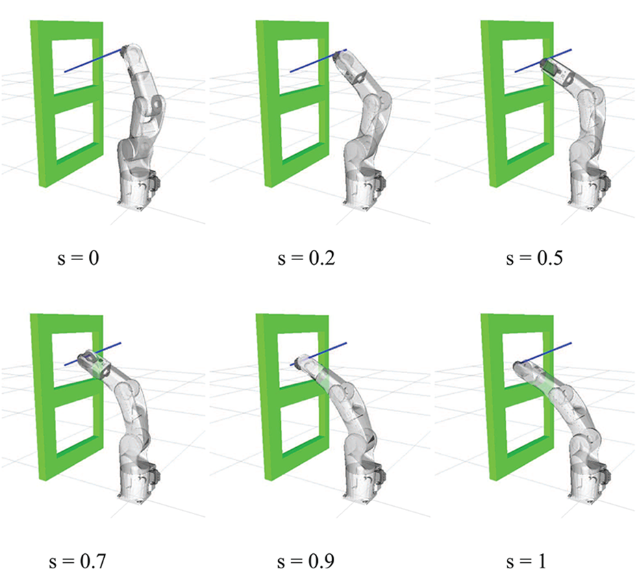
The first experiment (see Figure 4) is to plan a KUKA LWR manipulator to draw a specified arc in an environment with obstacles. In order to make the simulation more accurate, we build a simulation environment in MoveIt! using the URDF file of LWR robot and then add some obstacles. In high-dimensional space, collision detection is very challenging, so we use an open source library called Flexible Collision Library³³ which is supported by MoveIt!.

Figure 4.

A KUKA LWR manipulator draws a specified arc in the environment with obstacles. Six snapshots from a solution are shown and correspond to six states from s = 0 to s = 1 in turn.

In this experiment, for a 7-DOF robot we set q_b = (θ ₁, θ ₂, θ ₄) and q_r = (θ ₃, θ ₅, θ ₆, θ ₇). Meanwhile, the specified arc starts from coordinate (−0.5, −0.4, 0.7) to (0, −0.4, 0.8) and is represented as

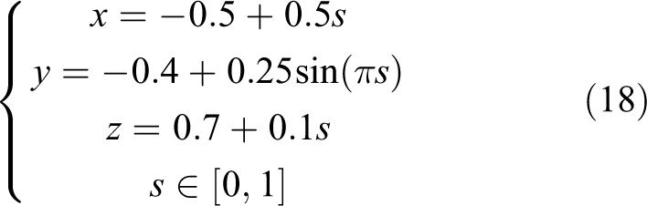
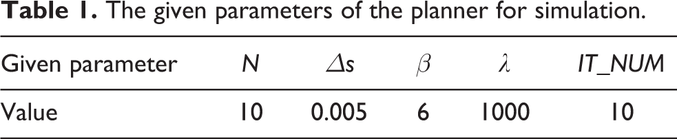
{\begin{matrix} x = - 0.5 + 0.5 s \\ y = - 0.4 + 0.25 sin (π s) \\ z = 0.7 + 0.1 s \\ s \in [0, 1] \end{matrix}

Table 1 gives the values of the parameters required in the planner. The explanation for these parameters is as follows.

N is the number of samples by equispacing the assigned task path and N + 1 leaves are created. The value of N usually depends on the length of the task path and it is similar to the incremental distance in traditional RRT algorithm. When the environment is relatively simple, a smaller value of N will speed up the trajectory search. However, when the environment is complicated, a larger value of N will make the manipulator easier to pass through some narrow space.

Δs is the integration step of Euler method which is used for motion generation between adjacent leaves. Since the mapping from joint space to task space is nonlinear, planning errors are unavoidable. A smaller value of Δs will reduce such errors.

β is the maximum allowed norm of the second term as a proportion of the norm of the first term in the rhs of equation (6). It corresponds to the parameter goal bias in traditional RRT algorithm. The larger the β, the faster the feasible space is explored. At the same time, it increases the redundancy of the planned joint path.

λ is the weight of the tracking error in the cost of configurations.

IT_NUM is the number of feasible solutions obtained by iterative optimization in Algorithm 1.

Table 1.

The given parameters of the planner for simulation.

Given parameter	N	Δs	β	λ	IT_NUM
Value	10	0.005	6	1000	10

Through simulation experiments, we get the operating states of the robot at different times in Figure 4. By performing a fifth-order polynomial programming on redundant coordinates q_r , we can get relatively smooth paths and geometric velocity in joint space as shown in Figure 5. At each stage of the planning, we set the starting acceleration and the ending acceleration to 0. So the planned geometric acceleration is continuous and we cannot guarantee the continuity of the jerk as shown in Figure 5. Here the velocity, acceleration, and jerk are geometric representations relative to the parameter Δs. In practical applications, considering the limitation of the maximum velocity or acceleration of each joint of the current manipulator, it only necessarily sets the parameter Δs to a suitable specific time interval for each stage. Figure 6 illustrates that the proposed algorithm can track the specified path well and the specific parameters are as follows.

Figure 5.

The four figures represent the planned path, geometric velocity, acceleration, and jerk in joint space. They will be real velocity, acceleration, and jerk when s = t.

Figure 6.

The above figure is tracking performances in task space and the below is the tracking errors of three dimensions.

We have obtained the averaged performance data after many experiments and compared with the Control_Based planner²³ and the RRT_Like planner.²¹ As presented in Table 2, for the RRT_Like planner, due to the linear connection between two admissible configurations, large task error is its main drawback. The tracking accuracy can be improved by increasing the number of path samples N. However, it will lead to an increase in execution time obviously. For the Control_Based planner, short execution time and relatively low task error are its main advantages. However, due to the existence of joint redundancy, the length of the planned joint path is relatively large. We propose an optimized planner based on the Control_Based planner. As the number of iterations (IT_NUM) increases, the values of task error and path length will decrease significantly. Experiments show that the optimized planner is asymptotically optimized and have better path performance compared to the previous algorithms.

Table 2.

The comparative experimental performance data (averaged).

	IT_NUM	Execution time (s)	Nodes in tree	Optimization times	Mean task error (mm)	Path length
RRT_Like	(N = 20)	4.72	571	0	14.5	25.8
RRT_Like	(N = 50)	26.72	3592	0	7.38	31.27
Control_Based	—	2.52	243	0	0.338	26.6
Optimized planner	1	6.58	282	38	0.248	23.254
	5	18.22	836	138	0.213	22.1
	10	25.31	1075	258	0.199	21.379
	30	37.91	1853	413	0.145	17.85

All of the italic entries highlight the best performance in the column.

A traditional 6-DOF robot moving following a straight line

We have also experimented on the traditional 6-DOF robot. Since the task constraints in this experiment are only position constraints, the 6-DOF robot is also redundant for this problem. We use the robot model of DENSO (Japan) to perform simulation experiments in ROS. The parameters N, Δs, IT_NUM, and λ are the same as those in Table 1.

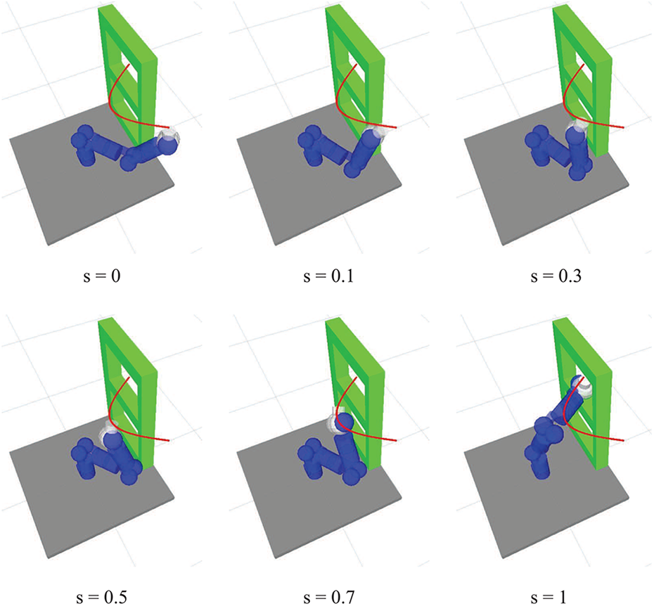
In this experiment, we set the tracking path to be a straight line from coordinate (0, −0.1, 0.9) to (0, −0.5, 0.75). Meanwhile, we set the first three joints as the base coordinates and the rest are redundant coordinates. The selection criterion for base coordinates is to ensure that the Jacobian matrix of the base coordinates is nonsingular. Then, the operating states are shown in Figure 7 and the proposed algorithm can generate a smooth joint path and track the specified trajectory well as shown in Figure 8.

Figure 7.

A DENSO manipulator draws a specified line in the environment with obstacles. Six snapshots from a solution are shown and correspond to six states from s = 0 to s = 1 in turn.

Figure 8.

The figure above is the joint space path and the below is tracking performance in task space.

Table 3 shows the effect of parameter β on path performance. When β = 0, the motion generation can only get a pseudoinverse solution without any self-motion in equation (4) and it usually cannot generate a feasible path in an environment with obstacles. Hence, the larger the β, the faster the feasible space is explored. However, when the value of β is too large, excessive self-motion will also reduce the path generation speed and it depends on the complexity of the current environment. Meanwhile, we can find that as parameter β increases, both the task error and the joint path length increase. In the case where the value of parameter IT_NUM is the same, the larger the β, the more obvious the optimization effect is. So for complex environments, when the parameter β needs to be large, the proposed algorithm will have better optimization effect.

Table 3.

The performance data as parameter β changes.

	β	Execution time (s)	Nodes in tree	Optimization times	Mean task error (mm)	Path length
Control_Based	0	>120	–	0	—	—
	4	0.18	27	0	0.03	8.787
	10	0.48	122	0	0.078	16.11
Optimized planner	4	0.82	211	69	0.012	6.767
Optimized planner	10	4.17	700	295	0.057	12.857

All of the italic entries highlight the best performance in the column.

Next, in order to reflect the optimization effect of the proposed algorithm, we set β = 10 and other parameters are the same as those in Table 1. We also compared the RRT_Like planner and the Control_Based planner as presented in Table 4. Since the 6-DOF manipulator is relatively simple, both in solving the Jacobian matrix and in the dimension of the configuration space, the planning speed is faster than the first experiment with LWR robot. Low tracking accuracy is still the main defect of the RRT_Like planner. By adjusting parameter IT_NUM to increase the number of iterations, we can get the performance data of the optimized planner as presented in Table 1. It is obvious that when the number of iterations increases, the optimization times will increase and then the path length decreases significantly. When IT_NUM $= 50$ , the path length in joint space is reduced by nearly 52% and the mean task error has been reduced to 0.0255 mm.

Table 4.

The performance data as parameter IT_NUM changes.

	IT_NUM	Execution time (s)	Nodes in tree	Optimization times	Mean task error (mm)	Path length
RRT_Like	(N = 20)	0.412	176	0	3.275	17.246
RRT_Like	(N = 50)	0.909	363	0	0.5857	17.901
Control_Based	—	0.48	122	0	0.0782	16.11
Optimized planner	1	0.423	89	6	0.0688	15.33
	10	4.17	700	295	0.047	13.19
	30	13.66	1555	1138	0.041	11.367
	50	21.65	2586	2891	0.0255	7.803

All of the italic entries highlight the best performance in the column.

A traditional 6-DOF robot tracking an irregular curve

To ensure the base coordinates q_b smooth, we assume that the task path is second-order continuous. In practical applications (e.g. welding), the task path is usually irregular and unsmooth. Here, we usually preprocess the task path in two ways. One is to split the task path into multiple smooth subpaths and plan the subpaths separately. The second is to uniformly sample the task path, and then use the least squares curve to fit the sampling points. In this experiment, we use the second.

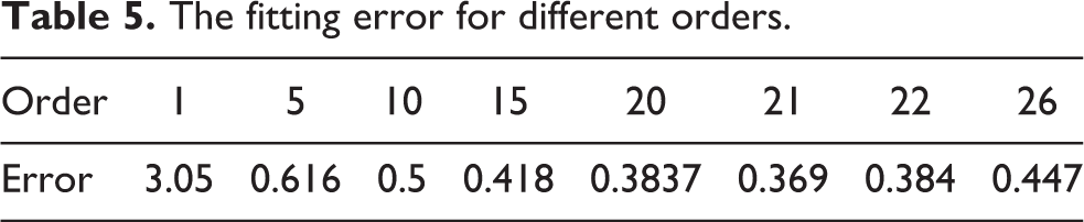
The experiment is to draw an irregular curve on a drawing board parallel to the x-axis as shown in Figure 10. We evenly sampled 56 points based on the y-axis and the fitting path is shown in Figure 9. We use polynomial for least squares curve fitting and the order is selected after multiple trials. As presented in Table 5, if the order is too small, the fitting error will be large, and if the order is too large, it will cause over-fitting. So in this experiment, we chose a polynomial with an order of 21.

Figure 9.

The above figure is the actual path in three dimensions and the below is a fitting curve for the sampling points.

Figure 10.

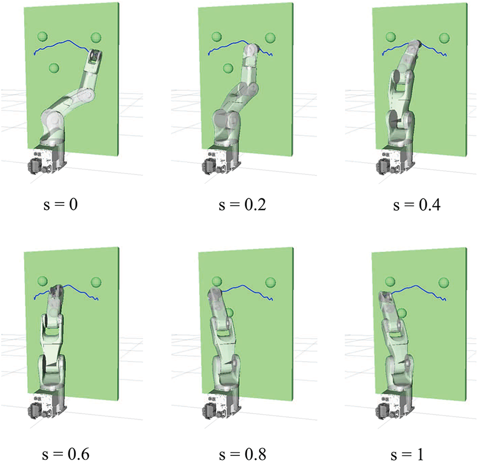
A DENSO manipulator draws an irregular curve on a drawing board. The green spheres are obstacles added in the environment.

Table 5.

The fitting error for different orders.

Order	1	5	10	15	20	21	22	26
Error	3.05	0.616	0.5	0.418	0.3837	0.369	0.384	0.447

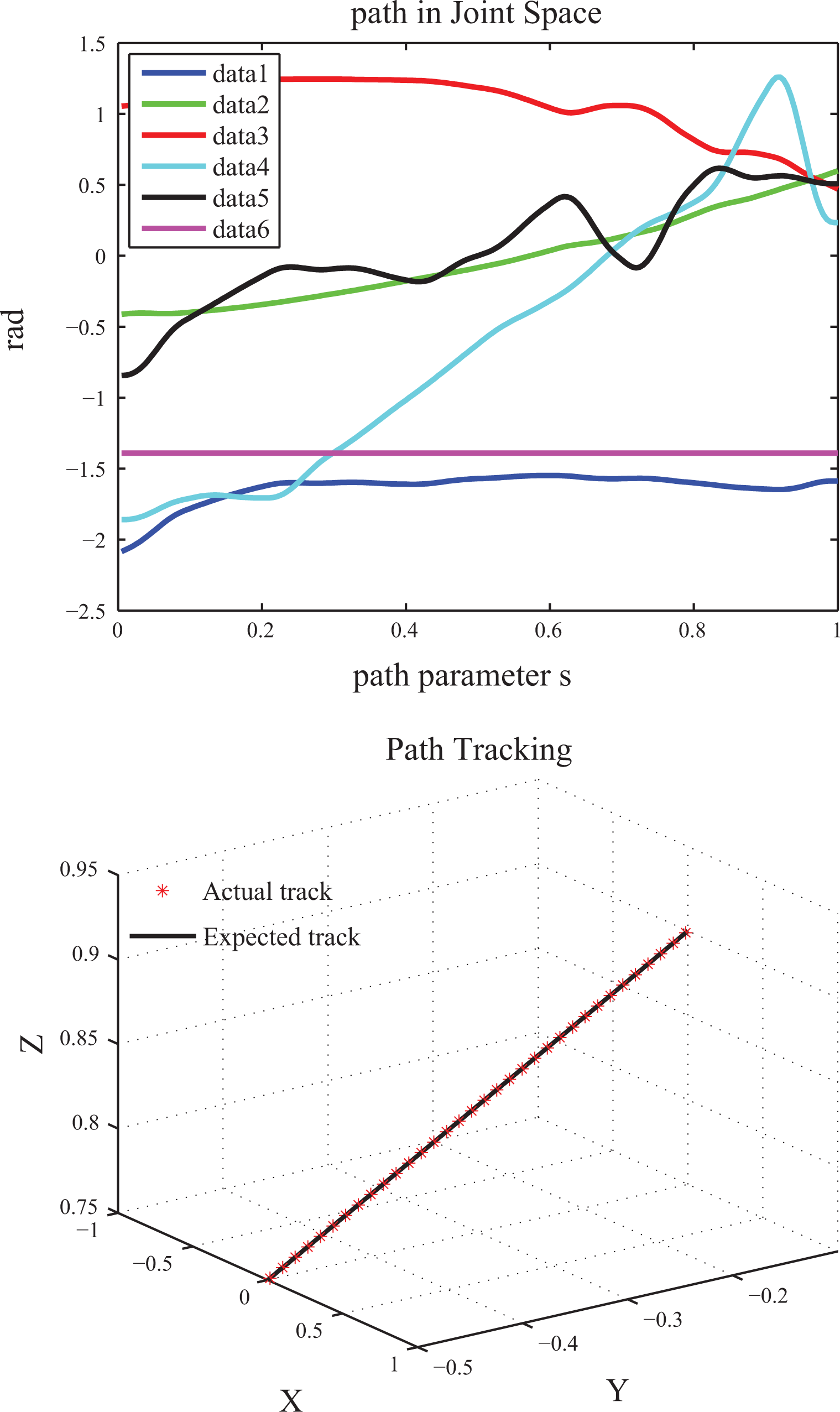
We have changed the environment and still use the robot model of the last experiment as shown in Figure 10. Then, we set β = 10 and other parameters are the same as those in Table 1. From Figure 11, we can see that the proposed algorithm can generate a smooth joint path. The use of curve fitting inevitably produces an error between the starting point of the fitted curve and the actual initial position of the robot end effector, so a certain tracking error is caused at the beginning of the planned trajectory and it will gradually decrease due to the error feedback mechanism as shown in Figure 11. Note that the tracking error or task error here is relative to the smooth path after fitting.

Figure 11.

The above figure is the joint space path and the below is the tracking errors of three dimensions.

As presented in Table 6, the mean task error is increased compared to the last experiment whose performance data are presented in Table 4. It can be seen that the smoothness and length of the tracking path have an impact on the tracking accuracy under the same experimental parameters. In practical applications, the values of Δs and N need to be adjusted to accommodate different end-effector paths. Similar to the previous experiment, the proposed optimized planner is far superior to the RRT_Like planner in tracking accuracy. At the same time, as the number of iterations increases, the planned joint path length will gradually decrease compared to the Control_Based planner. When IT_NUM $= 40$ , the path length in joint space is reduced by nearly 42%.

Table 6.

The performance data for tracking an irregular curve.

	IT_NUM	Execution time (s)	Nodes in tree	Optimization times	Mean task error (mm)	Path length
RRT_Like	(N = 20)	0.853	131	0	3.656	16.521
	(N = 50)	5.436	686	0	0.797	18.709
Control_Based	—	0.403	48	0	0.0908	15.384
Optimized planner	1	1.2	110	23	0.0852	14.255
	10	4.41	302	174	0.0802	13.53
	20	12.54	809	559	0.0745	12.39
	40	20.198	1563	1673	0.0448	8.863

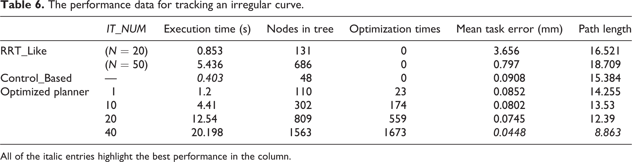
All of the italic entries highlight the best performance in the column.

Conclusion

For the problem of motion planning with task constraints, a sampling-based optimized algorithm has been proposed. In order to improve tracking accuracy, we apply kinematic control techniques and introduce negative feedback to the sampling-based algorithms. Then, by random self-motion in null space, the probabilistic completeness of the algorithm is ensured. Next, we adopt the reduced gradient method and perform a fifth-order polynomial programming on redundant coordinates to get a smooth path in joint space. Finally, we build an optimized structure similar to dynamic programming and it can generate an optimal path in joint space under the existing situation. So as new nodes are added, the resulting path is asymptotically optimized. There are several directions to improve the current work, such as:

attempt of generating an optimal subpath between adjacent leaves to achieve asymptotically optimality; and

dynamic adjustment of parameter β during path search.

Footnotes

Declaration of conflicting interests

The author(s) declared no potential conflicts of interest with respect to the research, authorship, and/or publication of this article.

Funding

The author(s) disclosed receipt of the following financial support for the research, authorship, and/or publication of this article: This work is supported by Major Science and Technology Project of Henan Province [Grant No. 161100210300].

ORCID iD

Kai Mi

Haojian Zhang

References

Chiaverini

Oriolo

Walker

. Kinematically redundant manipulators. In: Khatib

Siciliano

(eds) Handbook of robotics. Germany: Springer, 2009, pp. 245–268.

Hart

Nilsson

Raphael

. A formal basis for the heuristic determination of minimum cost paths. IEEE Trans Syst Sci Cybern 1968; 4(2): 100–107.

Khatib

. Real-time obstacle avoidance for manipulators and mobile robots. In: IEEE International Conference on Robotics and Automation, St. Louis, USA, 25–28 March 1985, pp. 500–505. Piscataway, NJ: IEEE.

Hoy

Matveev

Savkin

. Algorithms for collision free navigation of mobile robots in complex cluttered environments: a survey. Robotica 2015; 33(3): 463–497.

Wang

Zhu

Wang

. An improved artificial potential field method of trajectory planning and obstacle avoidance for redundant manipulators. Int J Adv Robot Syst 2018; 15(5): 1–13.

Ratliff

Zucker

Bagnell

. CHOMP: gradient optimization techniques for efficient motion planning. In: IEEE international conference on robotics and automation, Kobe, Japan, 12–17 May 2009, pp. 489–494. Piscataway, NJ: IEEE.

Kalakrishnan

Chitta

Theodorou

. STOMP: stochastic trajectory optimization for motion planning. In: IEEE international conference on robotics and automation, Shanghai, China, 9–13 May 2011, pp. 4569–4574. Piscataway, NJ: IEEE.

Mukadam

Yan

Boots

. Gaussian process motion planning. In: IEEE international conference on robotics and automation, Stockholm, Sweden, 16–21 May 2016, pp. 9–15. Piscataway, NJ: IEEE.

Kavraki

Svestka

Latombe

. Probabilistic roadmaps for path planning high-dimensional configuration spaces. IEEE Trans Robot Autom 1996; 12(4): 566–580.

10.

Lavalle

. Rapidly-exploring random trees: a new tool for path planning. Technical report, Department of Computer Science, Iowa State University, 1998.

11.

LaValle

Kuffner

. Rapidly-exploring random trees: progress and prospects. In: Workshop on algorithmic foundations of robotics, 2000.

12.

Kuffner

LaValle

. RRT-connect: an efficient approach to single-query path planning. In: IEEE international conference on robotics and automation, Piscataway, USA, 24–28 April 2000, pp. 995–1001. Piscataway, NJ: IEEE.

13.

Karaman

Frazzoli

. Sampling-based algorithms for optimal motion planning. Int J Rob Res 2011; 30(7): 846–894.

14.

Nasir

Islam

Malik

. RRT*-SMART: a rapid convergence implementation of RRT*. Int J Adv Robot Syst 2013; 10(7): 1–12.

15.

Klein

Huang

. Review of pseudoinverse control for use with kinematically redundant manipulators. IEEE Trans Syst Man Cybern 1983; 13(3): 245–250.

16.

Siciliano

. Kinematic control of redundant robot manipulators: a tutorial. J Intell Robot Syst 1990; 3(3): 201–212.

17.

Huang

Peng

Wei

. Clamping weighted least-norm method for the manipulator kinematic control: avoiding joint limits. In: 33rd Chinese control conference (CCC), Nanjing, China, 28–30 July 2014, pp. 8309–8314. Piscataway, NJ: IEEE.

18.

Huang

Peng

Wei

. Clamping weighted least-norm method for the manipulator kinematic control with constraints. Int J Control 2016; 89(11): 2240–2249.

19.

Martin

Baillieul

Hollerbach

. Resolution of kinematic redundancy using optimization techniques. IEEE Trans Robot Autom 1989; 5(4): 529–533.

20.

Mclean

Cameron

. The virtual springs method: path planning and collision avoidance for redundant manipulators. Int J Robot Res 1996; 15(4): 300–319.

21.

Oriolo

Ottavi

Vendittelli

. Probabilistic motion planning for redundant robots along given end-effector paths. In: IEEE/RSJ international conference on intelligent robots and systems, Lausanne, Switzerland, 30 September–4 October 2002, pp. 1657–1662. Piscataway, NJ: IEEE.

22.

Stilman

. Task constrained motion planning in robot joint space. In: IEEE/RSJ international conference on intelligent robots and systems, Vancouver, Canada, 24–28 September 2007, pp. 3074–3081. Piscataway, NJ: IEEE.

23.

Oriolo

Vendittelli

. A control-based approach to task-constrained motion planning. In: IEEE/RSJ international conference on intelligent robots and systems, St Louis, MO, USA, 10–15 October 2009, pp. 297–302. Piscataway, NJ: IEEE.

24.

Cefalo

Oriolo

Vendittelli

. Planning safe cyclic motions under repetitive task constraints. In: IEEE international conference on robotics and automation, Karlsruhe, Germany, 6–10 May 2013, pp. 3807–3812. Piscataway, NJ: IEEE.

25.

Oriolo

Cefalo

Vendittelli

. Repeatable motion planning for redundant robots over cyclic tasks. IEEE Trans Robot 2017; 99: 1–14.

26.

Luca

Oriolo

. The reduced gradient method for solving redundancy in robot arms. IFAC Proc Vol 1990, 23(8): 133–138.

27.

Oriolo

. Stabilization of self-motions in redundant robots. In: IEEE international conference on robotics and automation, 1994, pp. 704–709. Piscataway, NJ: IEEE.

28.

Ray

. Nonholonomic constraints. Am J Phys 1966; 34(5): 406–408.

29.

Deo

. Application of optimal damped least-squares method to inverse kinematics of robotic manipulators. Master’s Thesis, Department of Electrical and Computer Engineering, Rice University, Houston, TX, April 1991.

30.

Wenger

. Cuspidal and noncuspidal robot manipulators. Robotica 2007; 25(6): 677–689.

31.

Bellman

. Dynamic programming. Science 1966; 153(3731): 34–37.

32.

MoveIt! software. http://moveit.ros.org (accessed 5 June 2018).

33.

Pan

Chitta

Manocha

. FCL: a general purpose library for collision and proximity queries. In: IEEE international conference on robotics and automation, Minnesota, USA, 14–18 May 2012, pp. 3859–3866. Piscataway, NJ: IEEE.

A sampling-based optimized algorithm for task-constrained motion planning

Abstract

Keywords

Introduction

Related work

Preliminary material

Kinematics model

Problem formulation

Motion generation

Forward motion generation

Steering motion generation

Tree extension

Algorithm analysis

Probabilistic completeness

Algorithm optimization

Simulation results

A KUKA LWR manipulator drawing an arc

A traditional 6-DOF robot moving following a straight line

A traditional 6-DOF robot tracking an irregular curve

Conclusion

Footnotes

Declaration of conflicting interests

Funding

ORCID iD

References