Sage Journals: Discover world-class research

Abstract

The correlation between stability and energy variations in control strategies for a mobile base robot with manipulators subjected to external disturbances is introduced. The correlation results can be used to stabilize and control problems when a mobile base robot is subjected to various types of external disturbances. This is because different robot system energy values display different stability distribution curves. Mobile base robot stability based on varying system’s energy is described. Two control strategies, computed force/torque and adaptive compensators, are applied to minimize uncertainties accompanied by the robot’s movements. The two compensators are then compared by simulating applied external disturbances, such as mobile base tipping motion and load mass changes on the robot end-effector. A comprehensive comparison with other methods is also described. The proposed technique is a useful tool in the maintenance of the degree of control and stability of the system and has various applications in the mobile robot tasks including choosing and placing operations, maneuvering around the workspace with protruding obstacles on sinuous shape paths, and manufacturing tasks.

Keywords

Correlation (stability vs. energy variations)system energy function comparison (computed force/torque vs. adaptive compensators)external disturbances (base tipping motion,load mass changes)

Introduction

Mobile robots are a solution for transferring loads over large distances, such as from inventory to a robotically operated cell. This type of mobile manipulator has many applications for tasks such as choosing and placing operations, remote maintenance, hazardous material handling, and so on. The movements of a robot’s mobile base and its manipulators need to be coordinated in order to balance the system and execute the specified tasks harmoniously.

Among various research subjects about mobile base robot system, this article focuses on stability with manipulators subjected to external disturbances based on varying system mechanical energy. Literatures^{1

–24} show the current trends in the area of stability analysis for robot systems. Xiao and Ghosh¹ introduced a real-time planning and control for robot manipulators in a reconfigurable work-cell. Du Toit and Burdick⁵ described a partially closed-loop receding horizon control algorithm whose solution integrates prediction and estimation. Debanik⁶ developed a visibility map algorithm to generate a safe path for a three-dimensional congested robot workspace. Joshi and Desrochers⁷ and Dubowsky and Vance⁸ introduced stabilities of mobile robots based on geometrical analysis. Surdhar and White¹² addressed a development of a fuzzy-controlled manipulator using optical tip displacement feedback. Norouzi et al.²⁰ proposed an analytical strategy to generate stable paths for reconfigurable mobile robots such as those equipped with manipulator arms and/or flippers. Ning et al.²¹ introduced the collective behaviors of mobile robots beyond the nearest neighbor rules by applying an acute angle test-based interaction rule. Krid et al.²² developed an active anti-roll system and its associated controller for a high-speed and agile autonomous mobile robot. Kim et al.²⁴ proposed a design of a transformable mobile robot as a concept of hybrid-type mobile robot in order to enhance mobility.

Robot system stability is an open issue that requires further research while the system is subjected to various external disturbances. Diverse methods have been introduced to resolve this issue. However, few such methods explore the technique described in this article. This includes application of system energy function to stability analysis while mobile base robots with manipulators are subjected to external disturbances. This article presents correlation results between stability and energy variations in control strategies for a mobile base robot with manipulators subjected to external disturbances. A comprehensive comparison with other algorithms is described in the “Comprehensive comparison with other methods” section.

Figure 1 shows the overall robot system information flow where correlation between stability and energy variations is derived through the system’s energy function linked to the computed force/torque and the adaptive compensators. The article is organized as follows. The “Modeling and stability analysis based on varying system total mechanical energy” section first describes the modeling and dynamic equations of a mobile base robot with manipulators (including mobile base tipping movement). Next, the robot system energy function is derived to show the correlation between stability and energy variations. If system total energy is progressively decreased, then a set of system nonlinear differential equations will ultimately converge to an equilibrium state. From the Lyapunov direct method, a real-valued energy function for the robot system is obtained. The variation of that energy function can then be used to grasp the degree of robot system stability. In the “Computed force/torque compensator” and “Adaptive compensator” sections, algorithms for the computed force/torque and the adaptive compensators are described. Implementing practical nonlinear robot system control requires considering issues like external disturbances, unknown loads, computational complexity, parameter uncertainty, and so on. The computed force/torque compensator uses a function of error as a performance index to measure the system operation and modifies the force and torque to obtain a more optimum response. The adaptive compensator suppresses perturbations, compensates for system uncertainties, and follows the desired trajectories uniformly in all configurations by obtaining estimated values for the system parameters.

Figure 1.

Overall information flow of mobile base robot system.

In the “Results and comparisons” section, the two compensators in the “Computed force/torque compensator” and “Adaptive compensator” sections are applied to the selected mobile robot system to show the correlation between stability and energy variations. Simulations for comparing the two compensators are performed by applying external disturbances, such as base tipping motion and load mass changes on the end-effector, to the robot system. The “Results and comparisons” section also describes a comprehensive comparison with other methods. Conclusion and future works are described in the last section.

Correlation between stability and energy variations in control strategies for mobile robot subjected to external disturbances

To design a stabilizing control strategy, the correlation between system stability and energy variations under external disturbances is described. Robot stability is analyzed by varying system energy, where values of control variables composing the system energy function are fed from the computed force/torque and the adaptive compensators. Then, some examples are presented concerning base tipping motion and changes to load mass on the end-effector.

Modeling and stability analysis based on varying system total mechanical energy

Modeling and dynamic equations

The selected mobile base robot consists of rigid links, with two degrees of freedom, mounted on a base that moves in the x direction of a Cartesian coordinate frame and has the base tipping motion θ_b as shown in Figures 2 and 3. Figure 3 shows the mobile robot system including the tipping angle θ_b , where +|θ_b | represents the front wheel position when placed higher than the rear wheel position, and −|θ_b | represents the opposite case to the above +|θ_b | case.

Figure 2.

Mobile base robot with manipulators under external disturbances.

Figure 3.

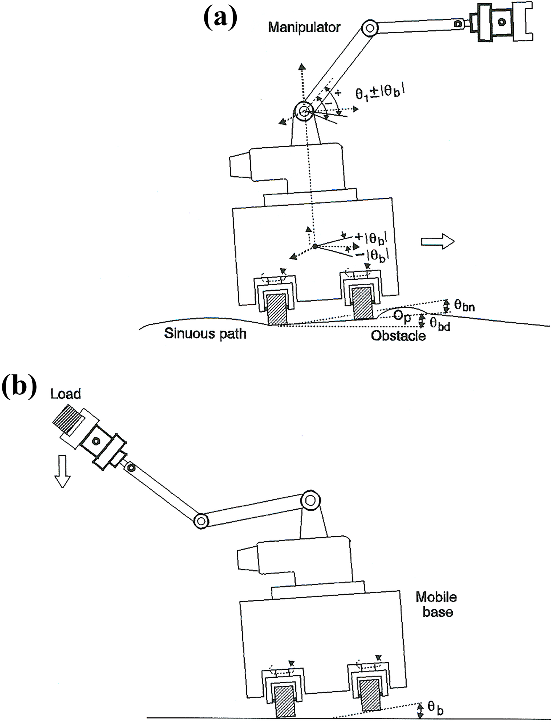
(a) θ_b _d (sinuous trajectory), θ_bn (tipping noise), and O_p (protruding obstacle) and (b) θ_b (tipping angle).

The dynamic equations of the selected robot system are obtained by the Lagrange–Euler equations²⁵

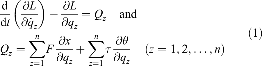
\frac{d}{d t} (\frac{\partial L}{\partial {\dot{q}}_{z}}) - \frac{\partial L}{\partial q_{z}} = Q_{z} and Q_{z} = \sum_{z = 1}^{n} F \frac{\partial x}{\partial q_{z}} + \sum_{z = 1}^{n} τ \frac{\partial θ}{\partial q_{z}} (z = 1, 2, \dots, n)

where q_z is the zth generalized coordinate. Q_z is the zth generalized force. L is the Lagrangian. x and θ are the translational and the rotational motion variables, respectively. F and τ are the force and the torque, respectively.

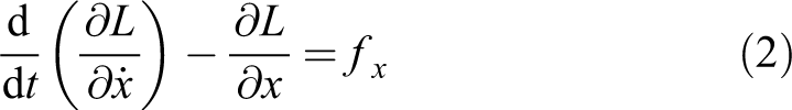
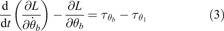
As an example of application for the Lagrange–Euler equations, some of the equation (1) for the selected robot system in Figure 2 are shown in equations (2) to (6). If the three coordinates (x, θ_b , θ ₁) among the generalized coordinates $q \in R^{4 \times 1}$ (=[x, θ_b , θ ₁, θ ₂]^T) are applied, then the Lagrange–Euler equations to the three variables are

\frac{d}{d t} (\frac{\partial L}{\partial \dot{x}}) - \frac{\partial L}{\partial x} = f_{x}

\frac{d}{d t} (\frac{\partial L}{\partial {\dot{θ}}_{b}}) - \frac{\partial L}{\partial θ_{b}} = τ_{θ_{b}} - τ_{θ_{1}}

\frac{d}{d t} (\frac{\partial L}{\partial {\dot{θ}}_{1}}) - \frac{\partial L}{\partial θ_{1}} = τ_{θ_{1}} - τ_{θ_{2}}

respectively, where the Lagrangian L is

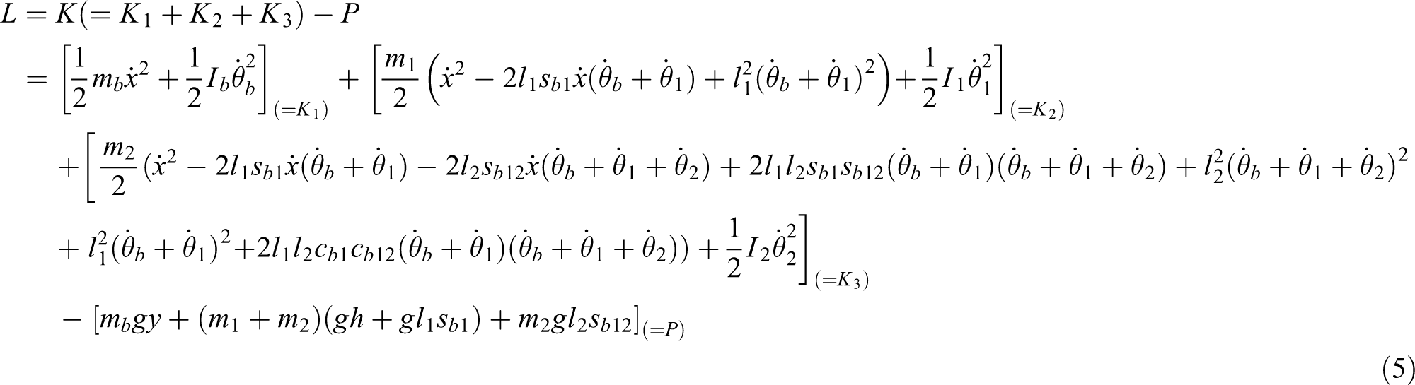
L = K (= K_{1} + K_{2} + K_{3}) - P = {[\frac{1}{2} m_{b} {\dot{x}}^{2} + \frac{1}{2} I_{b} {\dot{θ}}_{b}^{2}]}_{(= K_{1})} + [\frac{m_{1}}{2} ({\dot{x}}^{2} - 2 l_{1} s_{b 1} \dot{x} ({\dot{θ}}_{b} + {\dot{θ}}_{1}) + l_{1}^{2} {({\dot{θ}}_{b} + {\dot{θ}}_{1})}^{2}) {+ \frac{1}{2} I_{1} {\dot{θ}}_{1}^{2}]}_{(= K_{2})} + [\frac{m_{2}}{2} ({\dot{x}}^{2} - 2 l_{1} s_{b 1} \dot{x} ({\dot{θ}}_{b} + {\dot{θ}}_{1}) - 2 l_{2} s_{b 12} \dot{x} ({\dot{θ}}_{b} + {\dot{θ}}_{1} + {\dot{θ}}_{2}) + 2 l_{1} l_{2} s_{b 1} s_{b 12} ({\dot{θ}}_{b} + {\dot{θ}}_{1}) ({\dot{θ}}_{b} + {\dot{θ}}_{1} + {\dot{θ}}_{2}) + l_{2}^{2} {({\dot{θ}}_{b} + {\dot{θ}}_{1} + {\dot{θ}}_{2})}^{2} + l_{1}^{2} {({\dot{θ}}_{b} + {\dot{θ}}_{1})}^{2} {+ 2 l_{1} l_{2} c_{b 1} c_{b 12} ({\dot{θ}}_{b} + {\dot{θ}}_{1}) ({\dot{θ}}_{b} + {\dot{θ}}_{1} + {\dot{θ}}_{2})) + \frac{1}{2} I_{2} {\dot{θ}}_{2}^{2}]}_{(= K_{3})} - {[m_{b} g y + (m_{1} + m_{2}) (g h + g l_{1} s_{b 1}) + m_{2} g l_{2} s_{b 12}]}_{(= P)}

In equation (5), K (= K ₁ + K ₂ + K ₃) is the total kinetic energy of the selected system. K ₁, K ₂, and K ₃ are the kinetic energies of the mobile base, the lower arm, and the upper arm, respectively. P is the potential energy of the selected system. In equations (2) to (5) and Figures 2 and 3, m_b is the mass of the mobile base. m_i (i = 1, 2) is the mass of the ith arm. l_i is the length of the ith arm. h is the height from the x_w -axis to the origin of the lower arm. y is the height from the x_w -axis to the center mass of the mobile base. I_b , I ₁, and I ₂ are the mass moments of inertia of the mobile base, the lower arm, and the upper arm, respectively. x is the mobile base translational motion in the x_w direction. f_x and θ_b are the mobile base’s translation force and tipping angle. θ_i is the relative orientation angle of the ith arm with respect to the mobile base. $τ_{θ_{b}}$ , $τ_{θ_{1}}$ , and $τ_{θ_{2}}$ are the respective torques for the variables θ_b , θ ₁, and θ ₂ $θ_{2}$ . g is the gravitational constant. s_ijk and c_ijk are sin(θ_i + θ_j + θ_k ) and cos(θ_i + θ_j + θ_k ), respectively.

Equations (2) to (4) with the Lagrangian equation (5) give

\begin{array}{l} M_{11} \ddot{x} + M_{12} {\ddot{θ}}_{b} + M_{13} {\ddot{θ}}_{1} + M_{14} {\ddot{θ}}_{2} + U_{1} = f_{x} \\ M_{21} \ddot{x} + M_{22} {\ddot{θ}}_{b} + M_{23} {\ddot{θ}}_{1} + M_{24} {\ddot{θ}}_{2} + U_{2} = τ_{θ_{b}} - τ_{θ_{1}} and \\ M_{31} \ddot{x} + M_{32} {\ddot{θ}}_{b} + M_{33} {\ddot{θ}}_{1} + M_{34} {\ddot{θ}}_{2} + U_{3} = τ_{θ_{1}} - τ_{θ_{2}} \end{array}

respectively. The elements (M ₁₁, M ₁₂, M ₁₃, M ₁₄, M ₂₁, M ₂₂, M ₂₃, M ₂₄, M ₃₁, M ₃₂, M ₃₃, M ₃₄, U ₁, U ₂, and U ₃) in equation (6) are enumerated in equation (31).

From equation (1), the dynamic equations for the robot system can be written as

M (q) \ddot{q} + U (q, \dot{q}) = T

where $M (q) \in R^{n \times n}$ is the generalized inertia matrix. $\ddot{q} \in R^{n \times 1}$ is the generalized acceleration vector. $U \in R^{n \times 1}$ is the velocity coupling nonlinear vector. $T \in R^{n \times 1}$ is the generalized force or torque. Since $M (q) \in R^{n \times n}$ and $M^{- 1} (q) \in R^{n \times n}$ in equation (7) are not only symmetric and positive definite matrices but also constantly bounded for each generalized coordinate $q \in R^{n \times 1}$ , the generalized force or torque $T \in R^{n \times 1}$ in equation (7) can be replaced as follows

M (q) \ddot{q} + U (q, \dot{q}) = Ξ (q, \dot{q}, \ddot{q}) η (≐ T)

where $Ξ (q, \dot{q}, \ddot{q}) \in R^{n \times s}$ and $η \in R^{s \times 1}$ are known matrix functions and known system parameters, respectively. The elements of $Ξ (q, \dot{q}, \ddot{q})$ and η of equation (8) for the selected robot system in Figure 2 are described in equation (34) of the “Results of applied adaptive compensator” section.

Energy function of the robot system

The system energy function uses a nonlinear mass–damper–spring (MDS) system because its generalized concepts can be applied to a more complicated nonlinear system, such as the mobile base robot system described in the “Modeling and dynamic equations” section, and so on.

The continuous nonlinear MDS system dynamic equation can be represented as

m \ddot{x} + ϕ_{d} \dot{x} + κ_{s} x = 0

where m is the mass. x is a displacement of the mass m. $ϕ_{d} \dot{x}$ denotes nonlinear damping. κ_sx is a spring term. ϕ_d and κ_s are a damping coefficient and a spring stiffness constant, respectively. The total mechanical energy of the MDS system is

ϕ (x) = \frac{1}{2} m {\dot{x}}^{2} + \int_{0}^{x} κ_{s} x d x = \frac{1}{2} m {\dot{x}}^{2} + \frac{1}{2} κ_{s} x^{2}

where the first and the second terms are kinetic and potential energies of the system.

With equation (9), the energy variation rate of the MDS system can be obtained by derivativing equation (10) with respect to the displacement x as follows

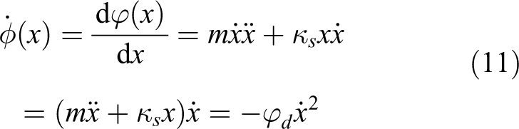
\begin{matrix} \dot{φ} (x) = \frac{d ϕ (x)}{d x} = m \dot{x} \ddot{x} + κ_{s} x \dot{x} \\ = (m \ddot{x} + κ_{s} x) \dot{x} = - ϕ_{d} {\dot{x}}^{2} \end{matrix}

A negative value in equation (11) means that the nonlinear MDS system’s energy is progressively decreased by the damper so that the system differential equation ultimately converges to its equilibrium state. In conclusion, if system total mechanical energy is progressively decreased, then a set of mechanical system nonlinear differential equations will ultimately converge to an equilibrium state. Therefore, mechanical system stability can be understood by considering system energy variation. The generalized concepts in this nonlinear MDS system can be applied to more complicated systems, such as robot systems, and so on.

Lyapunov’s direct method can be used to derive a real-valued energy function for nonlinear mechanical systems as below. It is assumed that there is a system, for example, such as equation (11), represented by a set of nonlinear differential equation whose generalized state space notation form is

\dot{x} (t) = g (x, t)

where x is a system state variable that belongs to Euclidean space Rⁿ . Then, some useful theorem and definition related to a stability of a system consisting of a set of nonlinear differential equations such as equation (12) are as follows.^26
–28

LaSalle’s theorem: Let Π be a bounded and closed set with the property that every solution of equation (12) which starts in Π remains for all future time in Π. Let $φ : Π \to R$ be a continuously differentiable function such that $\dot{φ} (x) \leq 0$ in Π. Let ϖ be the set of all points in Π, where $\dot{φ} (x) = 0$ . Let γ be the largest invariant set in ϖ. Then every solution starting in Π approaches γ as $t \to \infty$ .

Definition of GAS: If a positive definite function φ(x) is continuously partial derivatives and the derivative of φ(x) along all possible state trajectory of the nonlinear differential equation (12) is $\dot{ϕ} (x) \leq 0$ , then the function φ(x) becomes a Lyapunov function for equation (12). If there exists a real-valued function φ(x) with the following properties: (g ₁) φ(x) > 0; (g ₂) $\dot{φ} (x) < 0$ ; (g ₃) $φ (x) \to \infty$ as ∥x∥ → ∞, then the real-valued function φ(x) is globally asymptotically stable (GAS) at its equilibrium point.

From a stability perspective, the correlation between stability and mechanical energy of a robot system can be formulated as follows: (γ ₁) Convergence of the robot’s mechanical energy to zero implies an asymptotically stable system. (γ ₂) Zero energy of the mechanical system means equilibrium state. (γ ₃) System mechanical energy growth leads to an increase of the system instability. These relationships represent that system stability can be understood by considering the time variation of the system’s energy function. If mechanical system total energy is progressively diminished, then the mechanical system consisting of a set of nonlinear differential equations (equation (12)) will finally converge to an equilibrium state. Using Lyapunov’s direct method, a real-valued energy function for the robot system is generated. A variation of that energy function is then examined.

Based on the concepts and theories mentioned above, the energy function of the mobile robot system (a Lyapunov function candidate) is obtained as follows. A special case of the combined mobile base and manipulators is that first, the kinetic energy K_e of the mobile robot system can be written as

K_{e} = \frac{1}{2} {\dot{q}}^{T} M (q) \dot{q}

which is similar to $\frac{1}{2} m v^{2}$ that is kinetic energy of a system with a mass m and a velocity v. Next, the potential energy P_e of the system can be written as

P_{e} = \frac{1}{2} q^{T} k_{p} q

which is similar to $\frac{1}{2} κ_{e} x^{2}$ that is potential energy of a system with a coefficient of elasticity κ_e and a displacement x. In equations (13) and (14), q and $\dot{q}$ are actual position and velocity. k_p is a symmetric and positive definite matrix.

In a relationship between work and kinetic energy, if a force F with an acceleration a exerts on mass m of a particle, then an acceleration, an average speed, and a displacement of the particle are

\begin{matrix} a = \frac{Δ v}{Δ t} = \frac{v |_{t = x} - v_{0} |_{t = 0}}{t |_{t = x} - t_{0} |_{t = 0}} \\ v_{a v} = \frac{v + v_{0}}{2} and \\ x = x_{0} |_{t = 0} + v_{a v} t = x_{0} + \frac{v + v_{0}}{2} t \end{matrix}

respectively, where the initial values are v ₀ = 0, t ₀ = 0, and x ₀ = 0. Then, the work, W, done on the particle is equal to its gain in kinetic energy. That is

\begin{matrix} W = F x = max = m (\frac{v - v_{0}}{t}) (\frac{v + v_{0}}{2} t) \\ = \frac{1}{2} m v^{2} - \frac{1}{2} m v_{0}^{2} = \frac{1}{2} m v^{2} \end{matrix}

Lastly, the rate at which the force does work on the particle is

\frac{d W}{d t} = F v = \frac{d}{d t} (\frac{1}{2} m v^{2})

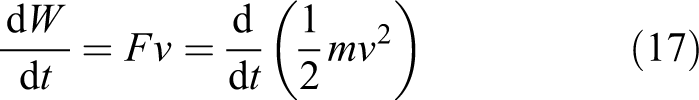
that is similar to $\frac{d}{d t} (K_{e})$ , where K _e is defined in equation (13). In equation (17), if the displacement variable x can be replaced by the generalized position variable q of a robot system, then F and v ( $= \frac{d x}{d t}$ ) correspond to T and $\dot{q}$ ( $= \frac{d q}{d t}$ ), respectively.

Based on the concepts in equations (15) to (17), a time change rate of the kinetic energy K _e, equation (13), in the mobile robot system is

\frac{d K_{e}}{d t} = {\dot{q}}^{T} T

From equations (13) to (14), the total mechanical energy of the mobile robot system is

Ψ (t) = \frac{1}{2} ({\dot{q}}^{T} M (q) \dot{q} + q^{T} k_{p} q) (= K_{e} + P_{e})

that is a Lyapunov function candidate. In equation (19), the first term is the kinetic energy of the mobile robot system as denoted in equation (13), and the second term is the potential energy of the system as denoted in equation (14).

With equation (18) and

\frac{d}{d t} (P_{e}) = \frac{d}{d t} (\frac{1}{2} q^{T} k_{p} q) = {\dot{q}}^{T} k_{p} q

the energy variation rate decreased by the mobile robot system is finally obtained as

\begin{matrix} \dot{Ψ} (t) = \frac{d Ψ (t)}{d t} = {\dot{q}}^{T} T + {\dot{q}}^{T} k_{p} q \end{matrix}

In equation (20), the real-valued energy function $\dot{Ψ} (t) < 0$ means that the energy is radiated from the mobile robot system that results in a decrease of the system’s mechanical energy leading to a stable system. Meanwhile, $\dot{Ψ} (t) > 0$ implies that the energy flows in the mobile robot system that results in a growth of the system’s mechanical energy leading to an unstable system. Based on these facts, the LaSalle’s theorem, the definition of GAS, and the relationships (γ ₁)–(γ ₃) mentioned above, the value of the energy function in equation (20) should be

\dot{Ψ} (t) (= {\dot{q}}^{T} T + {\dot{q}}^{T} k_{p} q) < 0

for a stable system. The values q, $\dot{q}$ , T, and k_p in equation (21) are fed from the two applied compensators (the computed force/torque and the adaptive compensators in the “Computed force/torque compensator” and “Adaptive compensator” sections) and the assumed trajectories equation (33). The criterion of the real-valued energy function in equation (21) can be used to understand the stability of the mobile robot system.

Computed force/torque compensator

The computed force/torque compensator utilizes an error function as a performance index to measure system operation and modifies the force and torque to obtain a more optimum response. The computed force/torque compensator overcomes robot system uncertainties in real time based on the system tracking performance.

The overall algorithmic flow of the computed force/torque compensator is shown in Figure 4(a). In Figure 4(a), θ_d and $θ \in R^{n \times 1}$ are the desired and the actual trajectories of the arm, respectively, where the subscript d in θ_d denotes desired. θ_bd and $θ_{b} \in R^{n \times 1}$ are the desired and the actual trajectories of the mobile base tipping motion. x_d and $x \in R^{n \times 1}$ are the desired and the actual trajectories of the mobile base translational motion.

Figure 4.

(a) Computed force/torque compensator and (b) adaptive compensator.

The above control variables are combined and used to derive requisite force and torque for the mobile robot system as follows

\begin{matrix} {\ddot{θ}}^{*} = {\ddot{θ}}_{d} + k_{v_{a}} ({\dot{θ}}_{d} - \dot{θ}) + k_{p_{a}} (θ_{d} - θ) \\ = {\ddot{θ}}_{d} + k_{v_{a}} {\dot{E}}_{a} + k_{p_{a}} E_{a} \\ {\ddot{θ}}_{b}^{*} = {\ddot{θ}}_{b d} + k_{v_{b}} ({\dot{θ}}_{b d} - {\dot{θ}}_{b}) + k_{p_{b}} (θ_{b d} - θ_{b}) \\ = {\ddot{θ}}_{b d} + k_{v_{b}} {\dot{E}}_{b} + k_{p_{b}} E_{b} \\ {\ddot{x}}^{*} = {\ddot{x}}_{d} + k_{v_{c}} ({\dot{x}}_{d} - \dot{x}) + k_{p_{c}} (x_{d} - x) \\ = {\ddot{x}}_{d} + k_{v_{c}} {\dot{E}}_{c} + k_{p_{c}} E_{c} \end{matrix}

whose generalized form is denoted as

{\ddot{q}}^{*} = {\ddot{q}}_{d} + k_{v} \dot{E} + k_{p} E \in R^{n \times 1} with q = [θ, θ_{b}, x]

In equations (22) to (23), the observed response error signal is generated by comparing the model output to the actual system output, which is often corrupted by noise, as shown in the following equation

\begin{array}{l} E_{a, b, or c} (= θ_{d} - θ, θ_{b d} - θ_{b}, or x_{d} - x) (≐ E) \in R^{n \times 1} and \\ {\dot{E}}_{a, b, or c} (= {\dot{θ}}_{d} - \dot{θ}, {\dot{θ}}_{b d} - {\dot{θ}}_{b}, or {\dot{x}}_{d} - \dot{x}) (≐ \dot{E}) \in R^{n \times 1} \end{array}

are the position and the velocity errors, respectively. ${\ddot{θ}}^{*} \in R^{n \times 1}$ is the arm acceleration input for calculating requisite torque. ${\ddot{θ}}_{b}^{*} \in R^{n \times 1}$ is the mobile base acceleration input related to the tipping motion for calculating requisite torque. ${\ddot{x}}^{*} \in R^{n \times 1}$ is the mobile base acceleration input related to the translational motion for obtaining requisite force. $k_{v_{a, b, or c}}$ and $k_{p_{a, b, or c}}$ are gain matrices associated with the speed of convergence to the desired motion.

The computed force/torque compensator updates the force and torque for all links of the mobile robot system through its own control routine, and the updated values are fed to equation (21).

Adaptive compensator

The adaptive compensator estimates the robot system parameters to compensate for uncertainties. If the estimated values of the system parameters are obtained, the effects of any uncertainties can then be minimized as the compensator minimizes the tracking error. Literatures providing adaptive routine examples are found in the literatures.^29

–33

The estimated equation of equation (7) is

\begin{matrix} T = \tilde{M} (q) {\ddot{q}}^{*} + \tilde{U} (q, \dot{q}) \\ = \tilde{M} (q) ({\ddot{q}}_{d} + k_{v} \dot{E} + k_{p} E) + \tilde{U} (q, \dot{q}) \end{matrix}

where ${\ddot{q}}^{*}$ $(= {\ddot{q}}_{d} + k_{v} \dot{E} + k_{p} E) \in R^{n \times 1}$ is the generalized driving acceleration input. $E (= q_{d} - q) \in R^{n \times 1}$ is the state variable error. k_v and $k_{p} \in R^{n \times n}$ are diagonal gain matrices. From equation (25), the error equation can be written as

\begin{matrix} \ddot{E} + k_{v} \dot{E} + k_{p} E = {\tilde{M}}^{- 1} ((M - \tilde{M}) \ddot{q} + U - \tilde{U}) \\ = {\tilde{M}}^{- 1} (M_{e} \ddot{q} + U_{e}) \end{matrix}

= {\tilde{M}}^{- 1} Ξ (q, \dot{q}, \ddot{q}) η

= {\tilde{M}}^{- 1} Ξ (q, \dot{q}, \ddot{q}) (P_{a} - {\tilde{P}}_{a}) (≐ {\tilde{M}}^{- 1} (q) T)

In equations (26) to (28), $M$ $-$ $\tilde{M}$ $(= M_{e}) \in R^{n \times n}$ and $U$ $-$ $\tilde{U}$ $(= U_{e}) \in R^{n \times 1}$ are modeling errors caused by parametric uncertainty. η $(= P_{a} - {\tilde{P}}_{a}) \in R^{s \times 1}$ is the system parameter error. P_a is the known nominal value of the system parameter. ${\tilde{P}}_{a}$ is the estimated value of P_a . s is the number of system parameters. Then, from equation (8), the system error equation (26) is replaced by equation (27). The elements of $Ξ (q, \dot{q}, \ddot{q}) \in R^{n \times s}$ and $η \in R^{s \times 1}$ of equation (27) in the selected mobile base robot system are shown in equation (34).

The servo error is determined as $E_{z} = \dot{E} + Γ E$ with a nonnegative diagonal matrix Γ. The state space form of equation (27) is represented as $\dot{x} = A x + B {\tilde{M}}^{- 1} Ξ η$ and $E_{z} = C x$ . There exist positive definite matrices P and Q such that $A^{T} P + P A = - Q$ A^TP + PA = −Q and PB = C ^T. A Lyapunov function candidate is determined as $ϖ (x, η) = x^{T} P x + η^{T} γ^{- 1} η$ with a positive definite diagonal matrix $γ \in R^{s \times s}$ .

\begin{matrix} \dot{ϖ} (x, η) = {\dot{x}}^{T} P x + x^{T} P \dot{x} + {\dot{η}}^{T} γ^{- 1} η + η^{T} γ^{- 1} \dot{η} \\ = - x^{T} Q x + 2 η^{T} (Ξ^{T} {\tilde{M}}^{- 1} E_{z} + γ^{- 1} \dot{η}) \\ = - x^{T} Q x + 2 η^{T} Δ \end{matrix}

where if choosing $Δ (= Ξ^{T} {\tilde{M}}^{- 1} E_{z} + γ^{- 1} \dot{η}) = 0$ , namely $\dot{η} = - γ Ξ^{T} {\tilde{M}}^{- 1} E_{z}$ , then equation (29) becomes $\dot{ϖ} (x, η) = - x^{T} Q x$ . Since the parameter error η is $P_{a} - {\tilde{P}}_{a}$ , thus $\dot{η} = - {\dot{\tilde{P}}}_{a}$ . Lastly, the adaptive rule, equation (30), modifies the system parameters

{\dot{\tilde{P}}}_{a} = γ Ξ^{T} {\tilde{M}}^{- 1} E_{z}

Figure 4(b) shows the overall information flow of the adaptive compensator, where meanings of the symbols, such as x_d , θ_d , θ_bd , $\dot{E}$ , and so on, are described in the “Computed force/torque compensator” section. The adaptive compensator updates the system parameters, the force, and the torque for all links of the mobile robot through its own control routine, and the updated values are fed to equation (21).

Results and comparisons

The above compensators are applied to the mobile robot system selected in the “Modeling and dynamic equations” section to show the correlation between stability and energy variations. A comparison of the two compensators is then described by simulating the applied external disturbances, such as mobile base tipping motion and load mass changes on the robot end-effector. In addition, a comprehensive comparison with other algorithms is described.

Results of applied computed force/torque compensator

The dynamic equations (equation (7)) of the selected mobile robot system, including the effects of both translational and tipping motions in Figures 2 and 3, are as follows. $M (q) \in R^{4 \times 4}$ is the generalized inertia matrix. $\ddot{q} (= [\ddot{x}, {\ddot{θ}}_{b}, {\ddot{θ}}_{1}, {\ddot{θ}}_{2}]^{T}) \in R^{4 \times 1}$ is the acceleration vector. $U (= [U_{1}, U_{2}, U_{3}, U_{4}]^{T}) \in R^{4 \times 1}$ is the velocity coupling nonlinear vector. $T (= [f_{x}, τ_{θ_{b}} - τ_{θ_{1}}, τ_{θ_{1}} - τ_{θ_{2}}, τ_{θ_{2}}]^{T}) \in R^{4 \times 1}$ is the generalized force and torque. The elements of M(q) and $U (q, \dot{q})$ are

\begin{array}{l} M_{11} = m_{b} + m_{1} + m_{2}, M_{12} = M_{21} = - m_{1} l_{1} s_{b 1} - m_{2} l_{2} s_{b 12} - m_{2} l_{1} s_{b 1} \\ M_{13} = M_{31} = - m_{1} l_{1} s_{b 1} - m_{2} l_{2} s_{b 12} - m_{2} l_{1} s_{b 1}, M_{14} = M_{41} = - m_{2} l_{2} s_{b 12} \\ M_{22} = (m_{1} + m_{2}) l_{1}^{2} + m_{2} l_{2}^{2} + 2 m_{2} l_{1} l_{2} (s_{b 1} s_{b 12} + c_{b 1} c_{b 12}) + I_{b} \\ M_{23} = M_{32} = (m_{1} + m_{2}) l_{1}^{2} + m_{2} l_{2}^{2} + 2 m_{2} l_{1} l_{2} (s_{b 1} s_{b 12} + c_{b 1} c_{b 12}) \\ M_{24} = M_{42} = m_{2} l_{2}^{2} + m_{2} l_{1} l_{2} (s_{b 1} s_{b 12} + c_{b 1} c_{b 12}) \\ M_{33} = (m_{1} + m_{2}) l_{1}^{2} + m_{2} l_{2}^{2} + 2 m_{2} l_{1} l_{2} (s_{b 1} s_{b 12} + c_{b 1} c_{b 12}) + I_{1} \\ M_{34} = M_{43} = m_{2} l_{2}^{2} + m_{2} l_{1} l_{2} (s_{b 1} s_{b 12} + c_{b 1} c_{b 12}), M_{44} = m_{2} l_{2}^{2} + I_{2} \\ U_{1} = - (m_{1} + m_{2}) l_{1} c_{b 1} {({\dot{θ}}_{b} + {\dot{θ}}_{1})}^{2} - m_{2} l_{2} c_{b 12} {({\dot{θ}}_{b} + {\dot{θ}}_{1} + {\dot{θ}}_{2})}^{2} \\ U_{2} = m_{2} l_{1} l_{2} s_{b 1} c_{b 12} {\dot{θ}}_{2} (2 {\dot{θ}}_{b} + 2 {\dot{θ}}_{1} + {\dot{θ}}_{2}) - 2 m_{2} l_{1} l_{2} c_{b 1} s_{b 12} {\dot{θ}}_{b} ({\dot{θ}}_{1} + {\dot{θ}}_{2}) \\ + (m_{1} + m_{2}) g l_{1} c_{b 1} + m_{2} g l_{2} c_{b 12} \\ U_{3} = m_{2} l_{1} l_{2} s_{b 1} c_{b 12} {\dot{θ}}_{2} (2 {\dot{θ}}_{b} + 2 {\dot{θ}}_{1} + {\dot{θ}}_{2}) + m_{2} l_{1} l_{2} c_{b 1} s_{b 12} (2 {\dot{θ}}_{b} + 2 {\dot{θ}}_{1} + {\dot{θ}}_{2}) \\ ({\dot{θ}}_{b} + {\dot{θ}}_{1} - 1) + (m_{1} + m_{2}) g l_{1} c_{b 1} + m_{2} g l_{2} c_{b 12} \\ U_{4} = m_{2} l_{1} l_{2} {({\dot{θ}}_{b} + 2 {\dot{θ}}_{1})}^{2} (c_{b 1} s_{b 12} - s_{b 1} c_{b 12}) + m_{2} g l_{2} c_{b 12} \end{array}

In the “Computed force/torque compensator” section and Figure 4(a), the state variable is defined as $X = [q^{T}, {\dot{q}}^{T}]^{T} = {[x, θ_{b}, θ_{1}, θ_{2}, \dot{x}, {\dot{θ}}_{b}, {\dot{θ}}_{1}, {\dot{θ}}_{2}]}^{T}$ with $q_{d} = [x_{d}, θ_{b d}, θ_{1 d}, θ_{2 d}]^{T}$ .

{\ddot{q}}_{i}^{*} = {\ddot{q}}_{d} + k_{v} \dot{E} + k_{p} E, (i = 1, \dots,4)

Equation (32) is the link driving acceleration input for calculating requisite force or torque, where $E (= q_{d} - q) \in R^{4 \times 1}$ is the state variable error, and k_v and $k_{p} \in R^{4 \times 4}$ are constant, diagonal gain matrices.

For the purpose of stability analysis, it is assumed that the mobile base and the arms follow preplanned trajectories. It first assumes that the mobile base tipping trajectory, θ_bd (t) in equation (33), can be generated as in the case when the mobile robot passes the sinuous shape path or the obstacle as shown in Figure 3(a). Next, the mobile base translational motion along the straight path, the mobile base tipping motion, the lower arm, and the upper arm move along the paths below

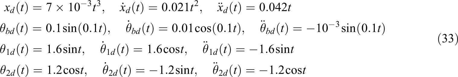
x_{d} (t) = 7 \times 10^{- 3} t^{3}, {\dot{x}}_{d} (t) = 0.021 t^{2}, {\ddot{x}}_{d} (t) = 0.042 t θ_{b d} (t) = 0.1 sin (0.1 t), {\dot{θ}}_{b d} (t) = 0.01 cos (0.1 t), {\ddot{θ}}_{b d} (t) = - 10^{- 3} sin (0.1 t) θ_{1 d} (t) = 1.6 sin t, {\dot{θ}}_{1 d} (t) = 1.6 cos t, {\ddot{θ}}_{1 d} (t) = - 1.6 sin t θ_{2 d} (t) = 1.2 cos t, {\dot{θ}}_{2 d} (t) = - 1.2 sin t, {\ddot{θ}}_{2 d} (t) = - 1.2 cos t

The system parameters are m_b =98.6 kg, m ₁ = 3.2 kg, m ₂ = 2.1 kg, l ₁ = 0.6 m, and l ₂ = 0.5 m.

Some results are shown in Figure 5, where the solid lines (a1) and (b1) in Figure 5(a) and (b) represent changes of the position errors of the mobile base translational motion (x) and the lower arm orientation angle (θ ₁), respectively. They are obtained using the computed force/torque compensator. The results indicate that the computed force/torque compensator minimizes the tracking errors.

Figure 5.

Position errors of (a) mobile base translational motion (x) and (b) lower arm orientation angle (θ ₁): [(a1/b1) Computed force/torque compensator and (a2/b2) adaptive compensator].

Results of applied adaptive compensator

The dynamic equation elements are described in equation (31). In the “Adaptive compensator” section and Figure 4(b), the state variable is the same one defined in the “Results of applied computed force/torque compensator” section, that is, $X = [q^{T}, {\dot{q}}^{T}]^{T} = {[x, θ_{b}, θ_{1}, θ_{2}, \dot{x}, {\dot{θ}}_{b}, {\dot{θ}}_{1}, {\dot{θ}}_{2}]}^{T}$ with $q_{d} = [x_{d}, θ_{b d}, θ_{1 d}, θ_{2 d}]^{T}$ . The link driving acceleration input in equation (25) is ${\ddot{q}}_{i}^{*} (= {\ddot{q}}_{d} + k_{v} \dot{E} + k_{p} E) \in R^{4 \times 1}$ , where $E (= q_{d} - q) \in R^{4 \times 1}$ is the control variable error, and k_v and $k_{p} \in R^{4 \times 4}$ are diagonal gain matrices. The estimated values of link parameters are ${\tilde{P}}_{a} = [{\tilde{m}}_{b}, {\tilde{m}}_{1}, {\tilde{m}}_{2}]^{T}$ The servo error is $E_{z} = \dot{E} + Γ E$ with a nonnegative diagonal matrix $Γ \in R^{4 \times 4}$ . From equation (27), the error equation is $\ddot{E} + k_{v} \dot{E} + k_{p} E = {\tilde{M}}^{- 1} Ξ η$ with ${\tilde{M}}^{- 1} \in R^{4 \times 4}$ . The elements $ξ_{i j}$ , $(i = 1, \dots, 4; j = 1, 2, 3)$ , of $Ξ (q, \dot{q}, \ddot{q}) \in R^{4 \times 3}$ and the link parameter errors $η \in R^{3 \times 1}$ for the selected mobile robot system shown in Figure 2 are as follows.

\begin{array}{l} ξ_{11} = \ddot{x}, ξ_{12} = \ddot{x} - l_{1} s_{b 1} ({\ddot{θ}}_{b} + {\ddot{θ}}_{1}) - l_{1} c_{b 1} {({\dot{θ}}_{b} + {\dot{θ}}_{1})}^{2} \\ ξ_{13} = \ddot{x} - (l_{1} s_{b 1} + l_{2} s_{b 12}) ({\ddot{θ}}_{b} + {\ddot{θ}}_{1}) - l_{2} s_{b 12} {\ddot{θ}}_{2} - l_{1} c_{b 1} {({\dot{θ}}_{b} + {\dot{θ}}_{1})}^{2} \\ - l_{2} c_{b 12} {({\dot{θ}}_{b} + {\dot{θ}}_{1} + {\dot{θ}}_{2})}^{2} \\ ξ_{22} = - l_{1} s_{b 1} \ddot{x} + l_{1}^{2} ({\ddot{θ}}_{b} + {\ddot{θ}}_{1}) + g l_{1} c_{b 1} \\ ξ_{23} = - (l_{1} s_{b 1} + l_{2} s_{b 12}) \ddot{x} + (l_{1}^{2} + l_{2}^{2}) {\ddot{θ}}_{b} + 2 l_{1} l_{2} (s_{b 1} s_{b 12} + c_{b 1} c_{b 12}) ({\ddot{θ}}_{b} + {\ddot{θ}}_{1}) \\ + (l_{1}^{2} + l_{2}^{2}) {\ddot{θ}}_{1} + l_{2}^{2} {\ddot{θ}}_{2} + l_{1} l_{2} (s_{b 1} s_{b 12} + c_{b 1} c_{b 12}) {\ddot{θ}}_{2} + l_{1} l_{2} s_{b 1} c_{b 12} (2 {\dot{θ}}_{b} + 2 {\dot{θ}}_{1} + {\dot{θ}}_{2}) {\dot{θ}}_{2} \\ - 2 l_{1} l_{2} c_{b 1} s_{b 12} ({\dot{θ}}_{1} + {\dot{θ}}_{2}) {\dot{θ}}_{b} + g l_{1} c_{b 1} + g l_{2} c_{b 12} \\ ξ_{32} = - l_{1} s_{b 1} \ddot{x} + l_{1}^{2} ({\ddot{θ}}_{b} + {\ddot{θ}}_{1}) + g l_{1} c_{b 1} \\ ξ_{33} = - (l_{1} s_{b 1} + l_{2} s_{b 12}) \ddot{x} + (l_{1}^{2} + l_{2}^{2}) {\ddot{θ}}_{b} + 2 l_{1} l_{2} (s_{b 1} s_{b 12} + c_{b 1} c_{b 12}) ({\ddot{θ}}_{b} + {\ddot{θ}}_{1}) \\ + (l_{1}^{2} + l_{2}^{2}) {\ddot{θ}}_{1} + l_{2}^{2} {\ddot{θ}}_{2} + l_{1} l_{2} (s_{b 1} s_{b 12} + c_{b 1} c_{b 12}) {\ddot{θ}}_{2} + l_{1} l_{2} s_{b 1} c_{b 12} (2 {\dot{θ}}_{b} + 2 {\dot{θ}}_{1} + {\dot{θ}}_{2}) {\dot{θ}}_{2} \\ + l_{1} l_{2} c_{b 1} s_{b 12} (2 {\dot{θ}}_{b} + 2 {\dot{θ}}_{1} + {\dot{θ}}_{2}) ({\dot{θ}}_{b} + {\dot{θ}}_{1} - 1) + g l_{1} c_{b 1} + g l_{2} c_{b 12} \\ ξ_{43} = - l_{2} s_{b 12} \ddot{x} + l_{2}^{2} ({\ddot{θ}}_{b} + {\ddot{θ}}_{1} + {\ddot{θ}}_{2}) + l_{1} l_{2} (s_{b 1} s_{b 12} + c_{b 1} c_{b 12}) ({\ddot{θ}}_{b} + {\ddot{θ}}_{1}) \\ + l_{1} l_{2} (c_{b 1} s_{b 12} - s_{b 1} c_{b 12}) ({\dot{θ}}_{b} + {\dot{θ}}_{1})^{2} + g l_{2} c_{b 12} \\ and all others ξ_{i j} = 0, (i = 1, \dots, 4 and j = 1,2,3), and \\ η = [m_{b} - {\tilde{m}}_{b}, m_{1} - {\tilde{m}}_{1}, m_{2} - {\tilde{m}}_{2}]^{T} \end{array}

The robot system parameters m_b , m ₁, and m ₂ shown in equation (34) are modified by the adaptive rule, equation (30), with a positive definite matrix $γ \in R^{3 \times 3}$ .

Similar to the “Results of applied computed force/torque compensator” section, it is assumed that the mobile base translational motion along the straight path, the tipping motion, the lower arm, and the upper arm follow the trajectories equation (33). The robot’s system parameters are also mentioned in the “Results of applied computed force/torque compensator” section. In the results shown in Figure 5, the dashed lines (a2) and (b2) in Figure 5(a) and (b) obtained by the adaptive compensator stand for position error variations of the mobile base translational motion (x) and the lower arm orientation angle (θ ₁), respectively. The results show that the adaptive compensator bounds the tracking errors.

Comparison of two compensators

Since the results described in the “Results of applied computed force/torque compensator” and “Results of applied adaptive compensator” sections show that both compensators minimize and bound the errors occurring when the mobile robot system follows the sinuous shape path shown in Figure 3(a), the subsequent types of external disturbances used in the comparison of the two compensators were applied to the robot system. Stability simulations are performed by applying an additional tipping disturbance noise to the mobile base following the desired trajectory, and by changing the load mass on the end-effector as follows.

Application of additional tipping disturbance noise: It is assumed that when the mobile robot passes a protruding obstacle with convex shape (O_p ) on a sinuous shape path θ_bd for a short time as shown in Figure 3(a), an additional tipping disturbance noise θ_bn can be generated, or the manipulators with the load on the end-effector heavily leaning to one side for a moment, as shown in Figure 3(b), can generate the tipping disturbance noise θ_bn . When additional tipping disturbance noises θ_bn (t) are applied at t = 5 and 5.9 s to the robot system that follows the trajectory θ_b _d(t) in equation (33), namely approximately 7.9° and 7.3° (generated from $θ_{b n} (t) = 0.14 sin (\frac{t}{3})$ at t = 5 and 5.9 s), respectively) are added to 2.7° and 3.1° (generated from θ_bd (t) in equation (33)) at t = 5 and 5.9 s, respectively, then the solid line (a) and the dashed line (b) in Figure 6 show energy variations of the robot system controlled by the computed force/torque and the adaptive compensators, respectively. The solid line pulses (a1) and (a2) in Figure 6 represent the sudden changes of the system energy when the front and the rear wheels of the robot system controlled by the computed force/torque compensator pass the protruding obstacle O_p at t = 5 and 5.9 s, respectively. Meanwhile, the dashed line pulses (b1) and (b2) in Figure 6 stand for the sudden changes of the system energy when the front and the rear wheels of the robot system controlled by the adaptive compensator pass the obstacle O_p at t = 5 and 5.9 s, respectively.

Figure 6.

Stability and energy variations for tipping disturbance noises $θ_{b n} (t {) |}_{t = 5 s} {= 7.9}^{\circ}$ and $θ_{b n} (t {) |}_{t = 5.9 s} {= 7.3}^{\circ}$ : (a) computed force/torque compensator and (b) adaptive compensator.

Among the four pulses (a1)–(b2) in Figure 6, the solid line pulses (a1) and (a2) generated by the tipping disturbance noises cross over the boundary ( $\dot{Ψ} (t) = 0$ ) of stable system though it is a very short time, the robot system is quickly restored to a stable state by the computed force/torque compensator. Meanwhile, the dashed line pulses (b1) and (b2) generated by the tipping disturbance noises are placed at more negative values (meaning more stable) and do not cross over the boundary line $\dot{Ψ} (t) = 0$ due to the advantages of the adaptive compensator’s algorithmic characteristics, in that, they can overcome various types of uncertainties. According to the results in Figure 6, the stability of the robot system is quickly restored to a stable state by satisfying the stability criterion equation (21) by the two compensators.

Application of load mass change: When the robot’s end-effector carries the loads with two different masses m_l = 1.4 and 2.9 kg, then the solid line curves (a1) and (b1) in Figure 7(a) and (b) represent energy variations of the robot system generated by the computed force/torque compensator for m_l = 1.4 and 2.9 kg, respectively. Meanwhile, the dashed line curves (a2) and (b2) in Figure 7(a) and (b) stand for energy variations of the robot system generated by the adaptive compensator for m_l = 1.4 and 2.9 kg, respectively. Figure 7(a) and (b) shows that the robot system is stabilized by the two compensators. But, due to the advantages of the adaptive compensator’s algorithmic characteristics described below, the dashed line curves (a2) and (b2) generated by the adaptive compensator are placed at more negative values (meaning more stable) than the solid line curves (a1) and (b1) generated by the computed force/torque compensator. In addition, Figure 7(b) shows that as the mass of load, m_l , increases to the maximum carrying capacity that the robot system can handle, both curves (b1) and (b2) place at more positive values (meaning less stable) and approach to the boundary ( $\dot{Ψ} (t) = 0$ ) of a stable system. According to the above results, the criterion of the real-valued energy function equation (21) can be utilized to grasp the degree of stability of the mobile robot system.

Results of comparison: While the computed force/torque compensator algorithm is much simpler than the adaptive compensator algorithm, the difference in the results received is not much since both compensators can successfully stabilize the mobile robot system when subjected to external disturbances. The advantage of the adaptive compensator over the computed force/torque compensator is that it uses the Lyapunov technique as a powerful stability tool, and the adaptive parameter scheme maintained high performance despite the changing system parameters. As the consequence, the adaptive compensator should have a higher rate of success than the computed force/torque compensator. However, the performance of the adaptive compensator can be affected by factors that include estimated values of known nominal values for system parameters, adaptive elements, and accurate system dynamics.

Figure 7.

Stability and energy variations for load masses (a) m_l = 1.4 kg and (b) m_l = 2.9 kg: (a1/b1) computed force/torque compensator and (a2/b2) adaptive compensator.

Comprehensive comparison with other methods

The global stability of mobile base robot is important, since a mobile robot base combined with manipulators carrying loads under various types of external disturbances should never tip over at any moment. Continued research endeavors^20

–24 have been made to improve the mobile robot system stability for various workplaces including manufacturing areas. As part of these research endeavors,^20

–24 proposed mobile robot stabilization techniques such as collective behaviors of mobile robots by applying an acute angle test-based interaction rule, active anti-roll system and its associated controller for autonomous mobile robot, and hybrid-type mobile robot to achieve better stability. However, their algorithms are limited on a local stability of robot systems and are accompanied with a high degree of computational complexity. These algorithmic characteristics certainly reduce the stability of the whole system.

Meanwhile, in this article, a system energy function, derived based on LaSalle’s theorem to ensure a global asymptotic stable system, as a powerful stability tool is used to analyze mobile base robot stability. The advantages of the method of system energy function are as follows. First, the proposed method maintains high performance despite effects of external disturbances as well as change of system dynamics; therefore, it should provide more stabilized robot system than the previous methods. Second, the proposed method can be not only a useful tool to grasp the degree of control system stability but also simply derived with relatively less computational complexity as described in the “Energy function of the robot system” section . This indicates significant improvement in the stability analysis of mobile robot systems, as illustrated in Figures 6 and 7.

Conclusion and future works

Contributions of this article are as follows. First, a system energy function is used to analyze mobile base robot stability. For a mobile base robot with manipulators subjected to external disturbances, the correlation between stability and energy variations in control strategies is described. The correlation results can be used to stabilize and control problems for mobile base robots subjected to various types of external disturbances. Second, the two applied compensators, the computed force/torque and the adaptive compensators, are compared through simulations performed by applying external disturbances to the robot system.

The results clearly show the correlation between stability and energy variations in the robot system. The proposed methodologies can be applied to a variety of robot tasks, such as choosing and placing, manufacturing, and controlling operations in workspaces with protruding obstacles on sinuous shape paths. The following should be addressed in as future works. It is necessary to extend the proposed technique to the stabilizing control problem for mobile base robots with manipulators subjected to external disturbances using more than four degrees of freedom in robot joint movements and different compensators such as robust and intelligent controllers.

Footnotes

Declaration of conflicting interests

The author(s) declared no potential conflicts of interest with respect to the research, authorship, and/or publication of this article.

Funding

The author(s) received no financial support for the research, authorship, and/or publication of this article.

ORCID iD

Changman Son

References

Xiao

Ghosh

. Real-time integration of sensing, planning and control in robotic work-cells. Control Eng Pract 2004; 12: 653–663.

Antonelli

Chiaverini

. A fuzzy approach to redundancy resolution for underwater vehicle-manipulator systems. Control Eng Pract 2003; 11: 445–452.

Zhang

Wei

. Dynamic balancing of robotic mechanisms via reconfiguration and integration design. Int J Robot Autom 2017; 32: 551–559.

Hakvoort

Aarts

Jonker

. Lifted system iterative learning control applied to an industrial robot. Control Eng Pract 2008; 16: 377–391.

Du Toit

Burdick

. Robot motion planning in dynamic, uncertain environments. IEEE Trans Robot 2012; 28(1): 101–115.

Debanik

. Algorithmic path planning of static robots in three dimensions using configuration space metrics. Robotica 2011; 29(2): 295–315.

Joshi

Desrochers

. Modeling and control of a mobile robot subject to disturbances. In: Proceeding IEEE international conference on robotics and automation, 7–10 April 1986, pp. 1508–1513.

Dubowsky

Vance

. Planning mobile manipulator motions considering vehicle dynamic stability constraints. In: Proceeding IEEE international conference on robotics and automation, 14–19 May 1989, pp. 1271–1276.

Son

. A stability analysis of a mobile base robot with an energy function. Int J Mach Tool Manu 1997; 337: 215–221.

10.

Son

. Stability analysis and motion planning strategies with fuzzy coordinator and learning for mobile base robotic part macro/micro-assembly tasks. Int J Mach Tool Manu 2004; 44: 1683–1695.

11.

Liu

Luo

Jia

. Acceleration analysis of multi-rigid-body systems and its application for parallel stabilized platform. Int J Robot Autom 2018; 33: 219–225.

12.

Surdhar

White

. A parallel fuzzy-controlled flexible manipulator using optical tip feedback. Robot Cim Int Manuf 2003; 19: 273–282.

13.

Gasparetto

Zanotto

. Technique for time-jerk optimal planning for robot trajectories. Robot Cim Int Manuf 2008; 24: 415–426.

14.

de Jesús Rubio

. Discrete time control based in neural networks for pendulums. Appl Soft Comput 2018; 68: 821–832.

15.

Dong

. Adaptive fuzzy neural network control for a constrained robot using impedance learning. IEEE Trans Neural Netw Learn Syst 2018; 29(4): 1174–1186.

16.

de Jesús Rubio

Garcia

Aquino

. Learning of operator hand movements via least angle regression to be teached in a manipulator. Evolving Syst 2018: 1–16. DOI: 10.1007/s12530-018-9224-1.

17.

Yen

Nan

Cuong

. Recurrent fuzzy wavelet neural networks based on robust adaptive sliding mode control for industrial robot manipulators. Neural Comput Appl 2018: 1–14. DOI: 10.1007/s00521-018-3520-3.

18.

de Jesús Rubio

. Modified optimal control with a back propagation network for robotic arms. IET Control Theory A 2012; 6(14): 2216–2225.

19.

Shao

. Robust adaptive control for coordinated constrained multiple flexible joint manipualtors with hysteresis loop. Math Probl Eng 2018; 2018: 1–9.

20.

Norouzi

Miro

Dissanayake

. Planning stable and efficient paths for reconfigurable robots on uneven terrain. J Intell Robot Syst 2017; 87(2): 291–312.

21.

Ning

Han

Zuo

. Collective behaviors of mobile robots beyond the nearest neighbor rules with switching topology. IEEE Trans Cybern 2018; 48(5): 1577–1590.

22.

Krid

Benamar

Zamzami

. Design of an active device for controlling lateral stability of fast mobile robot. Robotica 2016; 34(11): 2629–2651.

23.

Slawinski

Mut

. PD-like controllers for delayed bilateral teleoperation of manipulators robots. Int J Robust Nonlinear 2015; 25(12): 1801–1815.

24.

Kim

Jeon

Yang

. Design of a transformable mobile robot for enhancing mobility. Int J Adv Robot Syst 2017; 14(1): 1–14.

25.

Gonzalez

Lee

. Robotics: control, sensing, vision and intelligence. New York: McGraw-Hill, 1987.

26.

Friedland

. An introduction to state-space methods. New York: McGraw-Hill, 1986.

27.

Slotine

. The robust control of robot manipulators. Int J Robot Res 1985; 4: 49–64.

28.

Slotine

. Applied nonlinear control. Upper Saddle River: Prentice-Hall, 1991.

29.

Landau

Lozano

M’Saad

. Adaptive control: algorithms, analysis and applications. Berlin: Springer, 2011.

30.

Sastry

Bodson

. Adaptive control. Upper Saddle River: Prentice-Hall, 1989.

31.

Astolfi

Karagiannis

Ortega

. Nonlinear and adaptive control with applications. Berlin: Springer, 2010.

32.

Craig

Hsu

Sastry

. Adaptive control of mechanical manipulators. J Robotic Res 1987; 6: 16–28.

33.

Feng

Lozano

Adaptive control systems. Newnes, 1999.

Correlation between stability and energy variations in control strategies for mobile base robot with manipulators subjected to external disturbances

Abstract

Keywords

Introduction

Correlation between stability and energy variations in control strategies for mobile robot subjected to external disturbances

Modeling and stability analysis based on varying system total mechanical energy

Modeling and dynamic equations

Energy function of the robot system

Computed force/torque compensator

Adaptive compensator

Results and comparisons

Results of applied computed force/torque compensator

Results of applied adaptive compensator

Comparison of two compensators

Comprehensive comparison with other methods

Conclusion and future works

Footnotes

Declaration of conflicting interests

Funding

ORCID iD

References