Sage Journals: Discover world-class research

Abstract

This article presents a motion planning method for a novel hyper-redundant robot with minimal actuation based on the principles of fractals and self-organizing systems. The robot consists of multiple links connected by passive joints and a movable actuator. The actuator travels over the links to a given joint and adjusts the relative angle between the two adjacent links allowing the robot to undergo the same wide range of motions of hyper-redundant robot but with only one actuator. A suitable objective of the motion planner is to minimize the number of actuator traversals, which translates into minimizing the number of bends in the c-space trajectory. To this end, we propose a novel method for motion planning using fractals and self-organizing systems. A self-similar pattern for the path is implemented to map a path from start to finish. Each iteration of path segments is of smaller dimension than the previous one and is appended to it, just as in classical fractals. This process continues until a feasible trajectory is calculated. Self-organizing systems are then applied to this trajectory post-processing to optimize it by eliminating bends in the path. Examples of the robot maneuvering around obstacles and through confined spaces are shown to demonstrate the efficacy of the motion planner.

Keywords

Hyper-redundant robot fractal self-organizing system L-systems minimally actuated non-holonomic motion planning

Introduction

Hyper-redundant serial robots, or snake robots, have been the subject of extensive research over the past several decades.^1,2 Many different configurations and mechanisms have been proposed over the years, the principle motivation being their ability to navigate around obstacles and in highly confined spaces. Much effort has been put into increasing their speed and the forces they can exert while reducing their energy consumption.³

Yet, as challenging as the physical design of hyper-redundant robots is, planning their motions is an additional challenge.^4,5,6,7 Early motion planners for hyper-redundant robot motion planning were developed by Chirikjian.^8

–11 In those works, the curvature of the robotic snake is approximated as a continuous modal function with obstacles expressed as boundary constraints on the robot’s shape. Recent works have addressed obstacle avoidance schemes for hyper-redundant robots. State-of-the-art approaches including genetic algorithms,^12
–14 variational methods,^15,16 evolutionary algorithms,¹⁷ potential fields,¹⁸ and probabilistic road maps¹⁹ are used to plan the motions of the robots. Other sophisticated techniques are described by Pan and Yu²⁰ and Pan et al.²¹

Contemporary motion planners based on rapidly exploring random search trees work by having to “fill” an N-dimensional configuration space with nodes representing allowable robot configurations. Unfortunately, this becomes exponentially intractable for each additional robot link. To yield a feasible robot path in c-space within reasonable time, they must trade probabilistic completeness in favor of efficient runtime. In addition, only a small subset of the nodes constitute the optimal path.²² Recently, a specialized microprocessor was developed just to speed up the motion planning of a simple three-degree of freedom (DOF) industrial robot.²³

Yet, there is an even more fundamental modus operandi of contemporary robot motion planners: they sometimes attempt to find an optimal path, when in many practical applications, finding a mere feasible path is a sufficient challenge. This is especially true in medical and agricultural robotics, where a robotic manipulator must find any obstacle-free path through a tightly cluttered space. In fact, MacGregor and Chu²⁴ have shown that naive solutions for travelling salesman problems provided by untrained human subjects were often within 1% of the optimal solution. This fact calls the advantageousness of probabilistic algorithms into question and suggests that simpler methods be provided.

The particular high-dimensional motion planner that we are constructing has a unique constraint in that it is designed to plan the motions of the minimally actuated serial robot (MASR), described in detail by Mann et al.²⁵ The MASR is a planar serial robot consisting of multiple links connected by passive joints and of a small number of movable actuators, as shown in Figure 1. The actuators translate over the links to any given joint and adjust it to the desired angular displacement. The joint passively preserves its angle until it is actuated again.

Figure 1.

A two-dimensional prototype of the MASR. The robot in this figure has 10 links, one mobile actuator, and an end effector. The mobile actuator can freely travel over the links and rotates them upon command. MASR: minimally actuated serial robot.

As will be explained in section “Kinematic constraints,” the path of the MASR in c-space must be rectilinear, that is, consists of straight-line segments parallel with one of the N coordinate axis. An algorithm for a general two-link serial robot that yields a discretized rectilinear path is presented by Ahuactzin et al.^26,27 Known as Ariadne’s clew algorithm, it finds a rectilinear path (or Manhattan path) through obstacles for the robot by progressively exploring the solution space for landmark nodes and search for collision free Manhattan paths between the nodes.

Indeed, Ariadne’s clew algorithm addresses the aforementioned concerns about filling c-space by converting the motion planning problem into one of trajectory space, where the robot path is parameterized as a sequence of discrete angular movements. The algorithm then searches this trajectory space for a non-colliding Manhattan path. It returns such a path if it exists or terminates if it does not.

However, Ariadne’s clew algorithm would not be suited for finding paths for the MASR robot because the dimensions of the search space are multiplied by the number of discrete movements, or line segments, in the trajectory. This yields an explosively high-dimensional search space that is prohibitively intractable. Indeed, the examples of Manhattan paths shown by Mazer et al.²⁶ are only of two-DOF planar robots, and Mazer et al. admit²⁸ that the algorithm is not computationally capable of handling path planning for six-DOF industrial robots.

The problem of finding a feasible Manhattan path for the MASR is an example of the more general minimum bend rectilinear path problem. In this problem, the goal is to find a rectilinear path from start to finish between obstacles that has the smallest number of bends, that is, line segments in the path. It was first introduced by Lee.²⁹ However, it was shown by Fitch et al.³⁰ and Wagner³¹ to be non-deterministic polynomial (NP) complete for three dimensions or higher. This becomes all the more prohibitive for the high-dimensional c-space of the MASR.

To this end, we propose a motion planning method based on the self-similarity of fractals. The principle of this method is that the c-space trajectory from start to goal point should have the same pattern as a smaller scale trajectory around the obstacle, just as fractals have the same pattern at increasingly smaller scales. As will be explained in section “L-system description of path,” this yields a powerful robot motion planner with several distinct advantages such as scaling up very well to higher dimensions, relaxing the requirement to avoid obstacles, and avoiding the need to fill up high-dimensional space. And like other search-based motion planners, there is no need to precompute the obstacles or obtain any knowledge of their geometry or topology; only individual collision points along tentative paths need be considered.

This fractal-based method must be carried out by an algorithm that determines both the line segments of each iteration of the path and the size and location of each iteration of the fractalized path. The algorithm must be capable of searching the c-space for the best line segments while at the same time not wasting computing time on dead-end paths. Such an algorithm is described in sections “Fractal motion planner: Macro algorithm” and “Fractal motion planner: Path segment algorithm.”

While a non-colliding path is sufficient for the MASR, it is desirable to have one with as few line segments as possible. As explained in section “Kinematic constraints,” this corresponds to fewer translations of the actuator along the robot. A post-processing optimization procedure is thus presented in section “Self-organizing systems path improvement” that is based on self-organizing systems. It works by realigning nearby parallel line segments, thereby reducing the number of bends in the path. Examples that demonstrate the efficacy of the algorithm are shown in section “Examples,” and an analysis of the performance of the algorithm for higher dimensional configuration space is carried out in Appendix 1.

Mechanism description

The MASR robot system is composed of N links connected through passive joints, M < N mobile actuators that travel over the links and an end effector. The joints are passive in that there are no motors in between them while the angle between adjacent links is preserved by a passively locked spring. The number of links and mobile actuators can be easily varied depending on the proposed task. When a mobile actuator travels over the links, it can rotate the desired joint, thereby changing the relative angle between the links by a desired angle. The base is where the robot is connected to a constant support or a mobile platform. The robot is shown in Figure 1, while a detailed view of each link and the mobile actuator is shown in Figure 2. A more in-depth description and motivation for the MASR mechanism is provided by Shvalb et al.¹⁹

Figure 2.

(a) A top and bottom view of two adjacent links. (b) The mobile actuator that travels upon the links.¹⁹

For simplicity, we assume that each link is of uniform length L. The angle between the i-1th and ith serial link is denoted by θ_i (see Figure 1).

The orientation of each link in the plane is α_i , given by

α_{i} = \sum_{l = 1}^{i} θ_{l}

and the position of its end point is given by

(x_{i}, y_{i}) = (L \sum_{k = 1}^{i} cos (\sum_{l = 1}^{k} θ_{l}), L \sum_{k = 1}^{i} sin (\sum_{l = 1}^{k} θ_{l}))

The coordinate of the jth actuator is given by the pair (n_j , α_j ) $\in ℕ \times 1$ , where n_j is the link at which actuator j is currently located and α_j is the angle of the joint that the actuator is currently actuating. The latter has the same range as θ. We denote the set of actuated joints as J_A and the set of unactuated joints as J_U , given formally by

\begin{array}{l} J_{A} = {n_{1}, \dots n_{M}} \\ J_{U} = {1, \dots N} \ J_{A} \end{array}

Kinematic constraints

The configuration space of the robot, given that there are joint limits, is an N-dimensional cube I^N in the space of the N joint angles that define the state of the robot. However, the reduced actuation of the serial robot results in a very significant kinematic constraint. Only the joints upon which the actuator is situated may rotate, since they are intrinsically passive. 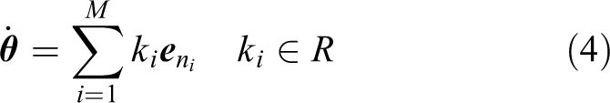For any given set of actuator locations n₁, n₂,…n_M , this means that the angular velocity of the joints $\dot{θ}$ can only be nonzero in those joint locations. In state-space, this corresponds to a tangent bundle confined to an M-dimensional plane embedded in R^N spanned by the unit vectors $e e_{n^{1}, n^{2},} \dots e_{n^{M}}$ given by

\dot{θ} = \sum_{i = 1}^{M} k_{i} e_{n_{i}} k_{i} \in R

Equation (4) represents a holonomic differential constraint, since it is a constraint on the time derivative of the coordinates and can be integrated to yield a constraint on the joint angles.³² This means that for any given actuator configuration, the motion of the robot is confined to an M-dimensional plane in c-space, translating the actuators of the robot thus corresponds to moving the manifold of feasible coordinates to a plane.

A visual example of this constraint for a three-DOF robot is shown in Figure 3. For a robot with two actuators, the motion is confined to a plane coincident with the surface of a hypercuboid. When the actuators switch to a different set of joints, the plane of feasible motion transfers to a different surface of the hypercuboid. For a robot with one actuator, the motion of the robot is confined to a one-dimensional “plane,” that is, a line parallel to one of the N axis. Whenever the single actuator switches to a different joint, the c-space motion switches to a different edge of the hypercuboid.

Figure 3.

The trajectory of the robots to traverse from initial configuration θ_A to final configuration θ_B in three-dimensional c-space. The trajectory of the fully actuated robot is represented by the black line; it has no spatial constraints. The trajectory of the two-actuator robot, shown by the green line segments, is confined to the surfaces of the hypercuboid shown in blue, and that of the one-actuator robot, shown by the red line segments, is confined to its edges.

We note that for simplicity, the rest of the article deals with an MASR that has only one actuator. The resulting trajectory of such a robot in c-space is a sequence of straight-line segments or a Manhattan path as in Mazer et al.²⁶ Devising a motion planner for MASR with two or more actuators is beyond the scope of this research.

The total time t _total required for the robot to reach a goal is thus comprised of the times required to rotate each joint plus the times required to traverse the actuator from one link to another plus a certain interruption delay between the translation and rotation. The latter two are a consumption of time unique to the MASR robot, and it is the price we pay for using less actuators than joints—there must be a “timeshare” of the actuator between the links.

Despite that limitation, it has been proven by Mann et al.²⁵ that the MASR can duplicate the geometric c-space path of a fully actuated robot with the same dimensions and DOFs to within any desired degree of accuracy. This means that if the motion of the latter is described by a parametric curve in c-space, then a curve representing the motion of the MASR in c-space can be constructed such that every point along it lies within a δ-norm of the latter. Moreover, given the error norm δ, the end point error of the MASR relative to the fully actuated robot was shown by Mann et al.²⁵ to lie within a well-defined range.

If we assume constant translational speed V of the mobile actuator and constant rotational speed ω, and that the delay is T _delay, then the time required to perform a task is

T_{TOTAL} = \frac{L \sum_{i}^{N_{STEP}} | Δ n_{i} |}{V} + \frac{\sum_{i}^{N_{STEP}} | Δ θ_{i} |}{ω} + N_{STEP} \times T_{delay}

where N _STEP is the total number of traversal steps, and Δn_i and Δθ_i are the respective number of links and rotation traversed during step i. These traversals of the actuator are the more time-consuming action, and it would, therefore, be desirable to minimize the number of traversals. This would constitute a suitable optimization goal of any motion planning algorithm for the MASR robot. Thus, minimizing the number of actuator traversals is equivalent to minimizing the time consumed by the motion planning task.

L-system description of path

Fractals for optimal path generation

The self-similarity of fractals inspires a powerful paradigm for motion planning. Fractals are iteratively constructed of simple geometric patterns at increasingly smaller scales. This suggests a general method for robot motion planning: generate simple paths from start to finish at increasingly smaller scales. In the same way that the fractal elements spawn several smaller elements of the same shape, each robot path could generate smaller “path-lets.”

The chief advantage of this strategy is to enable rapid motion planning for the MASR by iterating simple primitives instead of attempting to fill up c-space. While this principle would be useful for motion planning of any robot, it is particularly pertinent to the MASR because of the straight-line segments that constitute its trajectory. Its simplicity and geometric elegance make it a perfect candidate for the fractal approach.

However, there is a key factor in path-let generation for motion planning: obstacle avoidance. As opposed to classical fractals that generate smaller objects ad infinitum, the fractal approach to motion planning would generate path-lets from the larger path only when the latter collides with an obstacle. This connects the self-similarity of fractals to motion planning: each path has its own start and goal points. While the start and goal points of the initial, large-scale path coincides with the global start and goal robot configurations, those of the path-lets are the points which its parent path collides with an obstacle.

In other words, if a line segment collides with obstacles, a smaller-scale path from the start and end points of the segment will be generated. The goal of this path-let will be to circumvent this obstacle and avoid others as much as possible. If any of newly generated line segments of this path-let collide with an obstacle, they too will generate even smaller path-lets and so on until no more obstacles are encountered.

This process yields another distinct advantage: relaxation. The generated path-lets do not need to completely avoid obstacles. They are allowed to penetrate obstacles in the trajectory from start to goal and simply generate newer, smaller path-lets in an attempt to circumnavigate said obstacle. This saves considerable computation time while simultaneously allowing consideration of potential paths that standard optimization procedures would invalidate because of constraint violation.

The fractal generation method of motion planning is technically an example of multi-resolution motion planning. Multi-resolution methods are a broad approach to optimization problems and robot motion planning in particular. It works by calculating an optimal solution by first decomposing the search space into varying scales and then solving the planning problem on progressively smaller scales starting from a coarse scale.

Indeed, various implementations of multi-resolution methods have been used by many authors in robot motion planning. These methods variegate the resolution of the workspace, configuration space, time-axis, or a combination thereof.^32

–37 However, to the best of the authors’ knowledge, this is the first paper to use fractals as the multi-resolution building block for robot motion planning.

We first introduce the mathematical notation necessary to describe fractal motion planning, demonstrating that it is an instance of an L-system. We then develop the algorithm for generating complete paths using fractal generation in section “Fractal motion planner: Path segment algorithm.” Afterward in section “Self-organizing systems path improvement,” the heuristics for selecting the defining parameters of each individual path segment are detailed. Once a final path has been found, a methodology for further optimizing the path based on self-organizing systems is introduced in section “Examples.”

It must be emphasized that fractal motion planning is an incomplete algorithm, both in absolute and in probabilistic terms. There are quite a few obstacle situations where a path exists in c-space from start to finish but the fractal motion planner will fail to find it, no matter how fine the sampling resolution is. In addition, the analytical tools to analyze the convergence and computational runtime of the motion planning algorithm have not yet been developed. However, this article’s purpose is merely to demonstrate fractal motion planning as a proof of concept, a viable method for robot obstacle avoidance that is mathematically elegant and feasible. Further analysis of this method is a subject for future research.

L-system formulation of robot path

To begin generating the path of the MASR as a fractal, we must first describe the generation of paths in c-space as an L-system. An L-system is a formal grammar used to create strings that represent graphical objects based on production rules that expand symbols of an alphabet into a larger string of symbols. The reader is advised to review introductory material on fractals³⁸ to be familiar with the terminology of L-systems.

We start by defining the alphabet of the path generation system as consisting of four symbols:

U—a line segment that does not collide with any obstacles.

O—a line segment that collides with an obstacle.

s ₀ —the start point of the path.

f ₀ —the end point of the path.

This particular grammar is a parametric grammar, since two of the symbols, that is, line segments have several parameters associated with it:

s —the start point (in c-space) of the line segment.

f —the end point of the line segment.

v $\in {1, 2, \dots N}$ —the axis which the line segment is parallel to.

l—the length of the line segment.

p—the percentage of the line segment that collides with an obstacle (zero for U, nonzero for O).

c—the length along the line segment (percentagewise) at which the first collision occurs.

u —the last free sampled point along the line segment that occurs before the first collision (see section “Computing collision percentage and free points”).

The initiator, or axiom, of the L-system are the initial configuration and final configuration of the MASR. For simplicity, we formally define a complete path P as a string beginning with a start point, concluding with an end point, and containing a series of r line segments between them

P = {s_{0}, L_{1}, L_{2}, \dots, L_{r}, f_{0}}, L \in {O, U}

The production rules for the grammar is an algorithm that returns a path given an input set of letters. This production, which we label A, can occur in one of two modes:

producing a path between a start and end point, or

replacing a line segment with a path.

The first mode of production generates an initial path between two points. The second mode is based on a straightforward principle: Any line segment that collides with an obstacle must be replaced by a new series of line segments. This means that any time O is encountered, it must be replaced at the next iteration with a new path that attempts to circumvent the obstacle which O collides with. This is a very important aspect of relaxation—a path from start to finish may collide with obstacles on any given iteration, avoiding that obstacle is left to latter iterations (see Figure 4).

Figure 4.

The fractal motion planner creates a level 1 trajectory P1 1 from start to goal points (a). Each line segment that collides with COBS generates a second level path-let and to attempt to circumvent the obstacle (b). When no more line segment collides with obstacles, the path-lets merge with their parent path and the process is complete (c). The resulting Manhattan path will be post-processed to minimize bends in section “Self-organizing systems path improvement.”

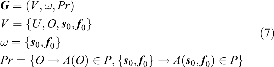
The L-system grammar G for production of paths may now be completely defined following classical L-system notation with an alphabet V, axiom ω, and production Pr:

\begin{array}{l} G = (V, ω, P r) \\ V = {U, O, s_{0}, f_{0}} \\ ω = {s_{0}, f_{0}} \\ P r = {O \to A (O) \in P, {s_{0}, f_{0}} \to A (s_{0}, f_{0}) \in P} \end{array}

Fractal motion planner: Macro algorithm

Definitions and notation

Constructing the production rules of P constitutes the essence of the fractal motion planner. The motion planner must be capable of selecting the “best” paths and line segments (what is defined as best will be explained shortly) and generate new path-lets for each line segment that collides. To accomplish this task, we introduce several new definitions and components of the motion planner:

The recursion level of a path-let and its respective start/end points is denoted by the superscript i and their serial number within the level by the subscript j, beginning with level 1. Thus, a path-let F_j ⁱ is the jth path of the ith level that starts at s _j ⁱ and finishes at f _j ⁱ . As with all fractals, level 1 contains only one path.

An incomplete path H is a series of r line segments that begins at s ₀ but does not (yet) end at f ₀

H = {s_{0}, L_{1}, L_{2}, \dots, L_{r}}, L \in {O, U}

A priority queue QU is a stack of currently incomplete paths, with the path containing the smallest number of collisions per unit length at the top of the stack.

A priority queue QF_j ⁱ is a stack of complete paths to be selected for the jth path-let of level i. As with QU, the path containing the smallest number of collisions per unit length is at the top of the stack.

The axis of an incomplete pathv(H) is the axis which its last line segment is parallel to—v(Lr) in the notation of section “L-system formulation of robot path.”

The recursion level of an incomplete path i(H) is the recursion level at which H is being constructed.

The size of an incomplete path z(H) is the number of line segments it contains.

The parent of a (in)complete path B(H) or B(F) is the collided line segment that generates the path-let H or F.

The path segment selector PS selects the next line segment, or several possible line segments, to append to an incomplete path, given the path-let’s goal end point f ₀ :

P S : H \times f_{0} \to L \in {O, U}

In other words, the selector extends an incomplete path by a single line segment to yield either an array of incomplete paths, or a complete path if the end point of the new line segment matches f ₀ ; the inner workings of PS are given in section “Self-organizing systems path improvement.”

Principles of the motion planning algorithm

The fractal motion planner consists of three principal steps:

selecting the best (i.e. fewest collisions per unit length) incomplete path to generate new incomplete/complete paths;

selecting the best complete path as the path-let from start to finish; and

generating new path-lets at smaller scale from each colliding line segment.

The process continues until there are no more colliding line segments. The output is a double array of complete paths divided among I iteration levels {{QF₁¹}, {QF₁ ², QF₂ ²,…QF_J2 ²},…,{QF₁ ^I, QF₂ ^I,…QF_JI ^I}}, where Ji is the maximum number of path-lets in level i. By definition, all path-lets in the last level I are collision free. This array can easily be converted into a collision-free path from the robot’s start to the goal point by replacing each O in QF_j ⁱ with its corresponding path-let in level j + 1, as will be shown in section “Examples.” A pseudocode of the motion planner is shown below as procedure FRACTAL-MOTION-PLANNER. A flowchart of the algorithm is shown in Appendix 1.

The variable J holds the number of path-lets for the current recursion level, while J_n is the number of path-lets in the next recursion level. The third while loop is the L-system aspect of the algorithm: it outputs a complete path from either a start/end point pair ( x _START and x _GOAL of the top recursion level) or from a collided line segment (O for all other recursions), thereby satisfying the production rules of equation (7). This is accomplished by using PS to compute the least-collided line segments and appends them to the current incomplete path H₀ to generate new paths. The new resultant paths that are incomplete are pushed into QU, while a path that is complete is pushed into QF_j ⁱ . There may be a multiple of line segments with the least collisions if several generated line segments do not collide with any obstacles, and so their collision percentage is obviously zero.

The search for the best path-let from the current s _j ⁱ to f _j ⁱ is concluded once there are no more incomplete paths left in QU or the number of complete paths in QF_j ⁱ have exceeded a certain amount. The latter can be set arbitrarily by the user as a constant or as a polynomial function of N. Once the best path-let is selected as P_j ⁱ , a pair of start/end points s ₀ , f ₀ are generated for every O within P_j ⁱ as a “placeholder” for a path-let in the next recursive level. The procedure terminates when there are no Os found in any P_j ⁱ within the current level.

Computing collision percentage and free points

Calculating the percentage that a line segment or path collides with obstacles is a straightforward calculation. For any given line segment L, K randomly generated sample points along the line segment are tested for collision. We reemphasize that there is no need to precompute the c-space obstacles; the individual collision points along the path segments are the only information about the obstacles necessary for fractal motion planning. The percentage of points that collide with an obstacle constitute the collision percentage of L. Label the colliding points x _O ₁, x _O2 ,… x _OC , and the non-colliding points x _N ₁, x _N2 ,… x _ND , C + D = K. The resulting collision percentage p of a path H_n that results from appending L to an existing incomplete path H₀ is yielded by adding the collision percentages of the former and latter weighted by their respective lengths

p (H_{n}) = \frac{l (L) p (L) + l (H_{0}) p (H_{0})}{l (L) + l (H_{0})}

The percentage c along L at which the first collision occurs is simply the length between s (L) and the closest collision point in units of L

c (L) = \frac{min_{i = 1, 2, \dots C} (‖ x_{O i} - s (L) ‖)}{l (L)}

The last free sampled point u along the line segment that occurs before the first collision is given by

u (L) = \underset{x_{N i}}{argmax} {\frac{(‖ x_{N i} - s (L) ‖)}{l (L)} | \frac{(‖ x_{N i} - s (L) ‖)}{l (L)} < c (L)}

The parameters c and u are essential for detecting corridors that cannot be circumnavigated, as described in section “Corridor detection.”

Fractal motion planner: Path segment algorithm

Optimal line segment criteria

Given a start point or path segment, determining what is the “best” line segment to continue the path is arguably the most delicate and tedious part of fractal motion planning. While classical fractals are simply scaled geometric objects, the pattern in fractal motion planning—a Manhattan path—has an infinite number of possible forms to take. Setting different criteria and parameters for the path segment computation will result in vastly different trajectories, many of which will not successfully reach the goal or avoid obstacles. The complication in line segment selection arises because the path of the MASR must meet three objectives:

search c-space for possible routes;

avoid obstacles as much as possible; and

reach the goal point.

However, there are several criteria that can be used to determine what the optimal line segment is to achieve these objectives. These criteria can provide a general guideline as to how to append a line segment depending on:

the recursion level,

the “parent” line segment that generated this path,

the current incomplete path H,

the goal point, and

the obstacle space.

The criteria and their effect on the optimal line segment computation are introduced informally, and then implemented into the path segment algorithm.

Direction

The next line segment of an incomplete path can point in any of 2N directions, where positive and negative advancement along each axis are counted as distinct directions. However, in order to search a new direction, it should be a different direction than that of the line segments from which it originated. This means that if it is not the first line segment of H, it should not be parallel to the axis v(H) of the line segment to which it is appended, and if it is the first, it should not be parallel to the axis v(B(H)) of its parent. On the other hand, in order to eventually reach the goal point, only the direction the points toward x _GOAL is examined. This means that for any axis v, only the direction of sign(x _GOAL ^v-x _START ^v) is examined, where x ^v is the vth coordinate of x . If start and end points have the same coordinate along v, then both ±v directions are examined. The unit vector corresponding to v is denoted by e _v .

Scale

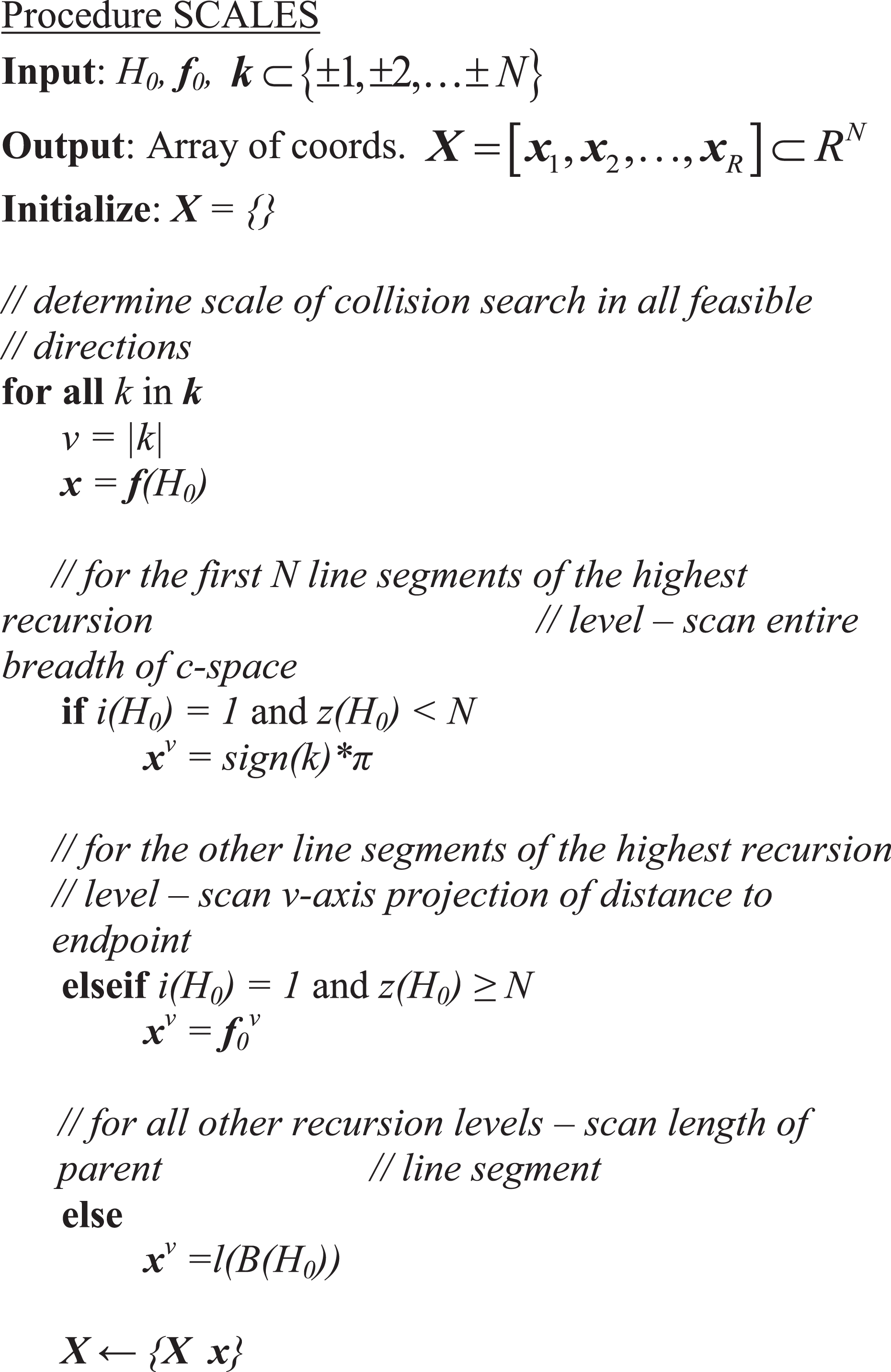
This is the critical component of the fractal approach to motion planning. Given the direction v, the length of c-space in that direction which will be sampled for collision is the scale of the path-let. This is analogous to the scale of a fractal iteration. As with fractals, the higher iteration numbers will have a smaller scale. However, we must achieve a balance between searching the space for feasible paths and reaching the goal. To this end, we propose the following heuristic for the ideal scale length d:

If it is the first iteration level and the number of line segments in H are less than N, then d = π, that is, the entire range of possible motion.

If it is the first iteration level and the number of line segments in H are more than or equal to N, then d = |v(x _GOAL )-v(x _START )|, that is, the projection of the distance between start and goal points on the v axis.

If it is the second or higher iteration level, then d = L(B(H)), that is, the length of the path-let’s parent.

Length

The length of the new line segment is calculated to maximize obstacle avoidance. This is accomplished by setting the end of the segment to be in the middle of the largest gap between obstacles, that is, the largest segment of C _FREE between x _START and x _START + de _v . Labeling X _N as the set of non-colliding points and X _O as the set of colliding points among the K samples taken, the cluster X _C is defined mathematically as

\begin{array}{l} X_{C} (v) = \underset{X \in P (X_{N})}{argmax {} | P (X) | | (x_{O}^{v} > sup_{x_{N} \in X_{N}} (x_{N}^{v})) \dots \\ o r (x_{O}^{v} < inf_{x_{N} \in X_{N}} (x_{N}^{v})) \forall x_{O} \in X_{O}} \end{array}

for a line segment parallel to the vth axis, where P(X) is the power set of X , and |P(X)| is its cardinality. The end point of the line segment would then be the centroid of X _C .

Corridor detection

Sometimes, however, circumventing obstacles does not work. Allowing path-lets to penetrate obstacles will not result in an obstacle-free path if the motion is confined to a corridor in c-space (see Figure 5). In this case, the entire paradigm of fractals for motion planning is moot, because the robot cannot navigate around obstacles, but rather is confined to navigating between obstacles.

Figure 5.

In this situation, the MASR’s trajectory is confined to moving between obstacles rather than around them. From the work of Bessiere et al.²⁷ MASR: minimally actuated serial robot.

However, we can add a crucial clause to the motion planning procedure to account for corridors. This clause does not entail scanning the entire c-space for obstacles or making any guesses about their topology. Instead, we use a simple heuristic based on an intuitive principle: a path inside a corridor is be tightly constrained on both sides of a given axis. This means that if the first collision on the new line segment occurs close enough to its start point, then the opposite direction must also be examined for collisions. If the first collision on the opposite direction also occurs close enough to the start point, then the direction with the first collision occurring farthest from its start point is used, with its end point equal to its last free point before its first collision point. Otherwise, the original direction is used.

The corridor detection module thus switches the mode of the motion planner from circumventing obstacles to remaining confined between obstacles. This corridor of confinement exists only relative to the given point and axis, that is, if both directions along the given axis encounter an obstacle within a small enough percentage of the line segment’s length, then a corridor is assumed to exist from the motion planner’s standpoint. The trajectory can then only proceed up to the last free point before this obstacle. The percentage is taken to be 10% in the implementation of the fractal motion planner.

Path segment algorithm pseudocode

The four modules described above will determine the direction, scale, length, and whether the path is in a corridor or not. The output of the combined modules will be a single or multiple of line segments that are appended to the current incomplete path, with the resulting path-let inserted into QU or QF_j ⁱ . The pseudocode for the entire path segment algorithm is shown below.

Self-organizing systems path improvement

Once the fractal path has been generated, it must be converted to a suitable MASR trajectory and then optimized to minimize actuator traversals by minimizing the number of line segments, that is, minimizing bends in the path. As mentioned in the Introduction, reducing the number of line segments in the MASR trajectory corresponds to fewer actuator translations along the links and thus a more rapid traversal from start to goal configuration. This form of path optimization occurs as a post-processing stage of motion planning. Decoupling the path optimization from the fractal motion planner provides a distinct advantage in that the L-system can generate a feasible path without being hindered by optimization considerations. This promotes calculation of a collision-free path in highly confined spaces where finding even a feasible trajectory is a challenge for a highly redundant robot.

The bends are minimized by an algorithm inspired by self-organizing systems, or self-assembly, found in nature.³⁹ For the MASR, each line segment is an element of the system. In order to reduce the number of line segments, each line segment shifts to the closest parallel line segment. If this shift can occur without colliding into any obstacles, then the two-line segments fuse into one, thereby reducing the total number of line segments, as shown in Figure 6. This process continues until there no more segments can be aligned.

Figure 6.

Original and optimized MASR trajectory. The two original line segments in the upper right corners (shown by the thin solid lines) shift to re-align with the nearest parallel line segments. Their new position is shown by the dashed lines. This reduces the total number of line segments in the trajectory from six to four.

However, as in any other algorithm, the mechanics of the self-organizing process must be precise. It must determine which of the two parallel line segments is to be shifted and how the surrounding line segments are to be moved, inserted, deleted, and renumbered. All of these parameters will be outlined in this section.

Trajectory reconstruction

Before reassembling the trajectory, it must be converted from fractal form to a single sequence of line segments. As described in section “Definitions and notation,” the fractal is described by a double array of path-lets. The trajectory can be constructed using a straightforward recursion that simply replaces each U in every path-let in the double array with its child path-let. The end result is a single sequence of non-colliding line segments U₁ , U₂ ,…, U_Z .

Rules for line segment realignment

Line segment shift

For any two parallel line segments that are to be realigned, one of them will shift while the other will remain stationary. Deciding which of the two will shift is determined probabilistically based on their relative lengths: the shorter line segment is more likely to shift, while the longer is more likely to remain stationary. Labeling the two parallel line segments U_j and U_k , their respective probabilities of shifting P(E_j) and P(E_k) are thus given by

\begin{array}{l} P (E_{j}) = \frac{d (U_{k})}{d (U_{j}) + d (U_{k})} \\ P (E_{k}) = 1 - P (E_{j}) = \frac{d (U_{j})}{d (U_{j}) + d (U_{k})} \end{array}

If the new position of the shifted line does not collide with any obstacles, then the realignment proceeds; otherwise, it is cancelled (see Figure 7).

Figure 7.

A pair of parallel line segments U_j and U_k within the trajectory. The probability of either one getting shifted to be collinear with the other is determined by their relative lengths.

Displacement of shifted line

For c-space of dimensions N ≥ 3, the parallel line segments U_j and U_k may be more than one segment apart, that is, k > j+1. This means that to realign, the shifting segment would have to cross over two or more line segments. To keep the realignment system simple, however, we allow each line segment to shift over only one other line segment. Therefore, for U_j and U_k parallel to axis v, the new coordinates of the shifted line segment U_j described by its respective start-point and end point s (U_j) and f (U_j) are given by

\begin{array}{l} s^{i} (U_{j}) \leftarrow f^{i} (U_{j + 1}) i \neq v \\ f^{i} (U_{j}) \leftarrow f^{i} (U_{j + 1}) \forall i \end{array}

If the shifted line segment is U_k , then they are correspondingly given by

\begin{array}{l} s^{i} (U_{k}) \leftarrow s^{i} (U_{k - 1}) \forall i \\ f^{i} (U_{k}) \leftarrow s^{i} (U_{k - 1}) i \neq v \end{array}

Rearrangement of surrounding line segments

Every time a line segment is shifted, it creates a gap between it and the preceding line segment (or the succeeding line segment if U_k is shifted). This gap must be filled with a new line segment U_N that satisfactorily connects between U_j-1 and the shifted U_j (or between U_k and U_k+1 if U_k is shifted). In addition, the line segment that was passed over for shifting must be deleted. The parameters of U_N where U_j is shifted are given by

\begin{array}{l} v (U_{N}) = v (U_{j + 1}) \\ s (U_{N}) = f (U_{j - 1}) \\ f (U_{N}) = s (U_{j}) \\ U_{j + 1} \leftarrow {} \end{array}

If it is U_k that is shifted, then the new line segment will have corresponding parameters described by

\begin{array}{l} v (U_{N}) = v (U_{k - 1}) \\ s (U_{N}) = f (U_{k}) \\ f (U_{N}) = f (U_{k + 1}) \\ U_{k - 1} \leftarrow {} \end{array}

Renumbering of line segments

After every realignment, the line segments must be renumbered sequentially to account for the line shift. If U_j and U_k are collinear, then they are fused into one line segment U_k , thereby reducing the total number of line segments in the trajectory. The numbering would then be U₁ , U₂ ,…, U_j-1 , U_N , U_k ,…, U_Z . On the other hand, if they are not collinear, then the numbering will be U₁ , U₂ ,…, U_j-1 , U_N , U_j , U_j+2 ,…, U_k ,…, U_Z .

Flow control of loop

The realignment process checks sequential parallel line segments for every axis v. For example, if there are Z line segments parallel to the vth axis, then the procedure will check for realignment between U_(1)v and U_(2)v , U_(2)v and U_(3)v ,…, and U_(Z-1)v and U_(Z)v , where U_(i)v is the ith line segment in the trajectory parallel to the vth axis.

This process continues from the beginning of the trajectory for every axis. If there are no more non-colliding segments for any axis, then the process restarts, because realigned line segments parallel to one axis alter the trajectory such that the alignment procedure for line segments parallel to a different axis may yield different results. In other words, two sequential parallel line segments within the current trajectory may not be realigned due to obstacle collision. However, the realignment process for a different axis restructures the trajectory (according to equation (17)), and so the two line segments might possibly be realigned this time around.

Pseudocode for realignment procedure

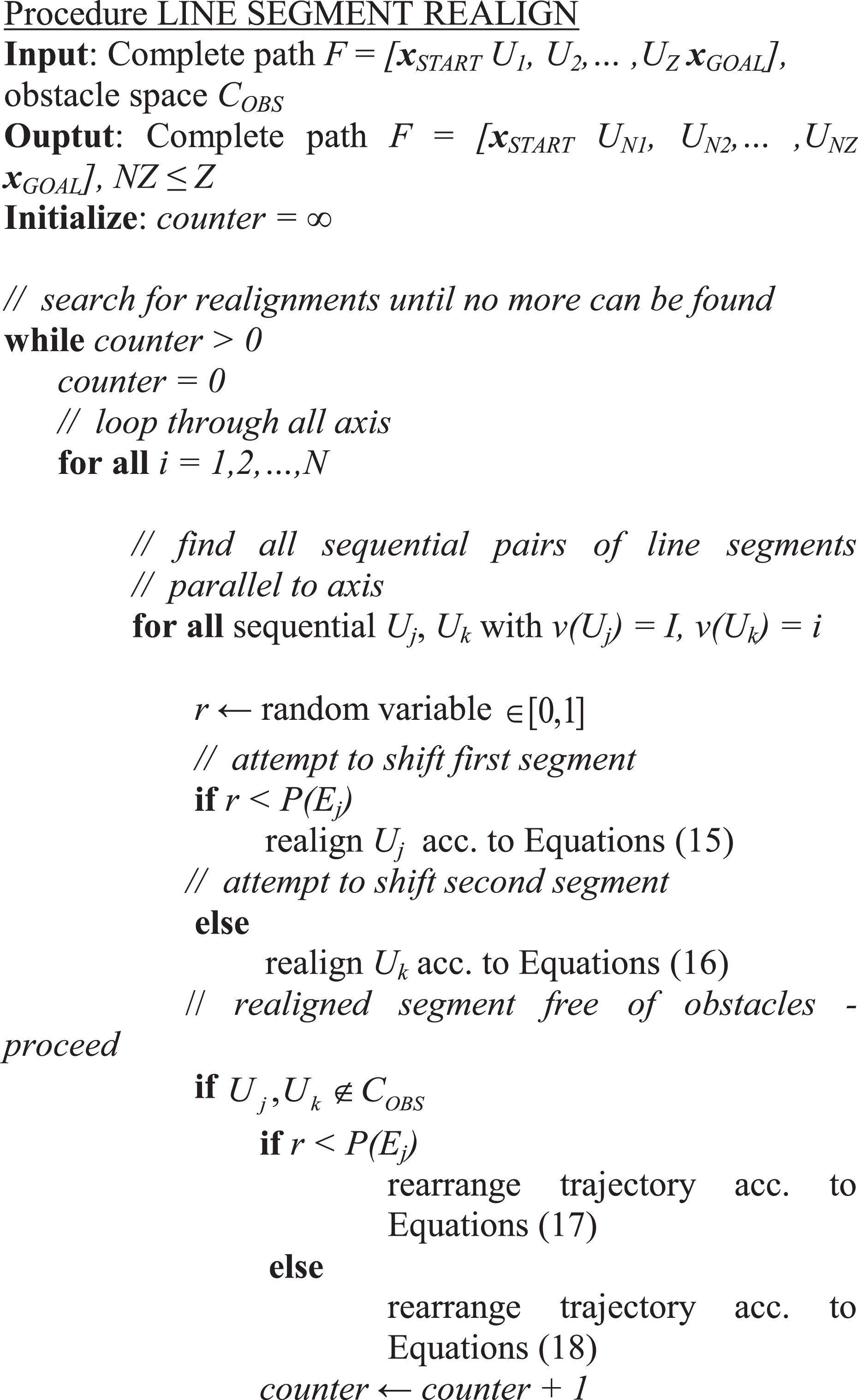
Based on the aforementioned criteria and heuristics, the pseudocode for realigning the line segments is presented below. The variable counter holds the number of line segment realigned during any given run. It is reset to zero once all axis and all realignments parallel to the given axis are checked for collision. The algorithm will terminate if it does not find any non-colliding realignments at all. The result is a trajectory with likely far fewer line segments than the original trajectory. The MASR robot can then proceed from start to finish in shorter time and fewer actuator translations.

Examples

We illustrate the performance of fractal motion planning with several examples of a simulated planar serial robot. The robot consists of three links connected passively and actuated by a single motor. Each link is 10 cm from joint to joint and 1 cm wide. The simulated environment consists of obstacles which the robot must avoid as it finds a path from start to finish. Demonstrating the results of the motion planner on the actual experimental MASR is an ongoing research project currently underway.

While the principles of fractal motion planning can be scaled up to higher DOF, we limit the examples in this research to robots with three-DOF. This allows the generated fractal path-lets and the self-organizing path optimizer to be visualized graphically. And although in principle, the fractal motion planner can work for higher dimensions, the simulation environment used (MATLAB 2013) did not promote the necessary calculations to be carried out in reasonable time. Adjustments can be made to the motion planner that shorten its runtime by further limiting the sizes of the path-lets and priority queues, but that is beyond the scope of this article.

The results of the fractal motion planner can be summed up by their computation time, the number of fractal levels, the number of actuator translations (both before and after the self-organizing system reduction), and the total angular displacement undergone by the actuator. These results are summarized in Table 1. Note that the computation times are significantly longer than those of comparable motion planning algorithms in current robotics literature. While this may prima facie cause some consternation regarding the efficacy of fractal motion planning, this was a result of the fact that the algorithm was not optimized at the micro-level, that is, arrays were used to store path structures rather than binary trees and the robot collision detection method was somewhat crude. In a more rapid development environment, we believe that computing time consumed by the fractal method for robot motion planning would be competitive with other motion planners and can be practically implemented in very high DOF robots.

Table 1.

Results of simulations

	Computation time (s)	Number of fractal layers	Original number of actuator translations	Final number of actuator translations	% Reduction	Total angular displacement (°)
Example 1	70.4	1	15	14	6.67	514.5
Example 2	144.3	5	32	12	68.7	385.9
Example 3	36.8	2	13	6	53.85	610.5

Example 1

In this first example, the MASR must insert itself into a narrow slanted passageway. The fractal motion planner successfully guides the MASR into the passageway, as shown in Figure 9. Only one recursion level is necessary here. For this example, the algorithm detected a corridor, and directed the MASR accordingly. The final c-space trajectory is shown in Figure 8. Note that the obstacle space, sampled by the red dots in the figure, was not computed in advance; it is illustrated in order for the reader to visualize the path circumnavigating around the obstacles.

Figure 8.

C-space trajectory of MASR robot navigating between obstacles, denoted by the red dots. All angles are expressed in radians. MASR: minimally actuated serial robot.

Figure 9.

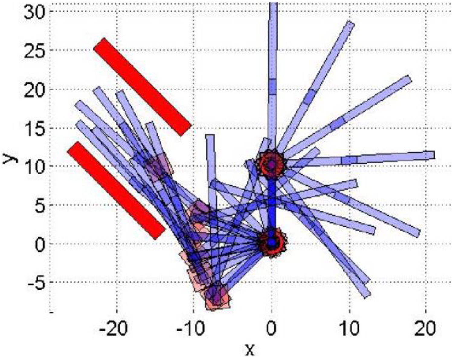
Snapshots of the MASR robot entering into a narrow passageway. The actuator must translate 14 times to accomplish this task. Due to its ability to translate, one actuator is sufficient to accomplish the task. MASR: minimally actuated serial robot.

Example 2

Here, the MASR must pass into an opening between two L-shaped obstacles. The snapshot of motion is shown in Figure 10. This particular motion plan consisted of five fractal recursion levels. The fractal path-lets of all levels are shown in Figure 11. Each path-let was generated to circumvent an obstacle. Apparently, the self-organizing path optimization procedure was very effective in reducing the total number of actuator translations, as the original number of 32 before the procedure was reduced to 12, a 68% reduction!

Figure 10.

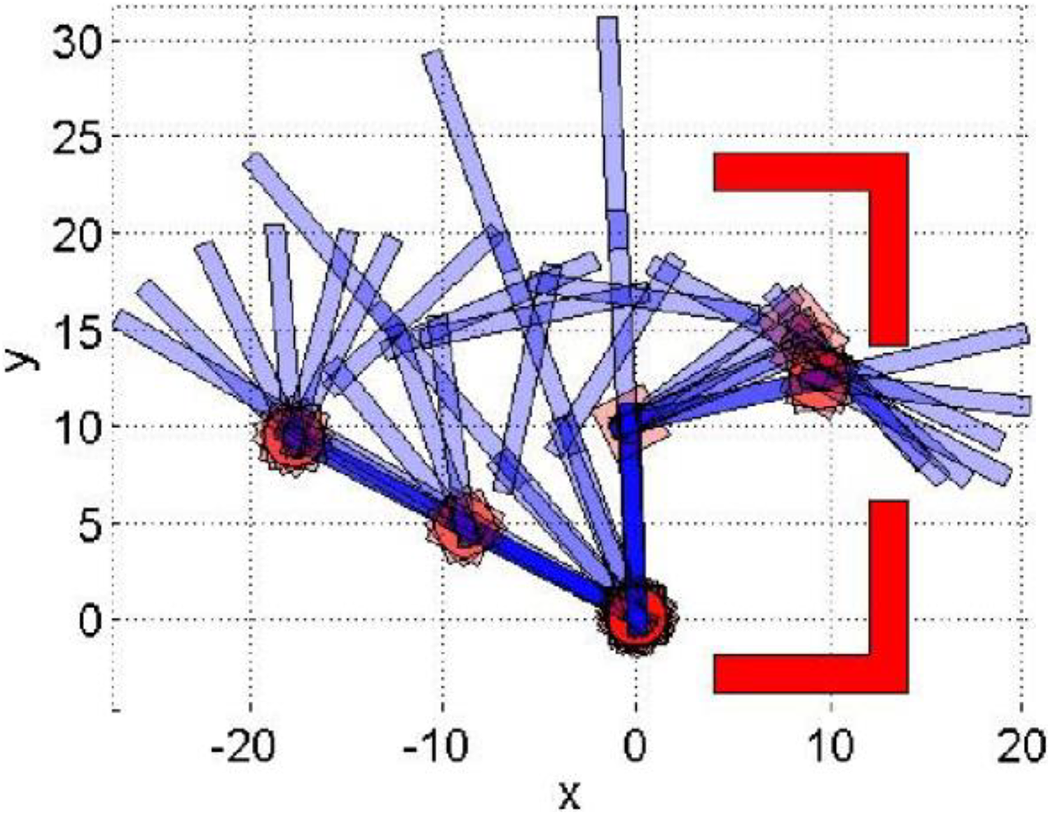
Snapshots of the MASR passing around obstacles trajectory. This requires 12 actuator translations. MASR: minimally actuated serial robot.

Figure 11.

Recursion levels of fractals in c-space that are incorporated into trajectory. The start and end points are shown by the black knobs.

Example 3

In this final example, the MASR navigates around several obstacles from start to finish. Snapshots of the robot throughout its traversal are shown in Figure 12. The fractal motion planner generated two recursion levels in the course computing this trajectory. The self-organizing procedure further reduced the number of actuator translations to six. The final c-space trajectory is shown in Figure 13.

Figure 12.

Snapshots of the MASR passing around obstacles. MASR: minimally actuated serial robot.

Figure 13.

C-space trajectory of MASR robot navigating between obstacles. MASR: minimally actuated serial robot.

Summary and conclusions

This article has introduced a novel method for motion planning of minimally actuated hyper-redundant robots around obstacles based on fractals and self-organizing systems. The method consists of constructing a Manhattan path for the robot from start to finish that minimizes exposure to obstacles. Each line segment on this path that collides with an obstacle generates another smaller scale path-let, just as in classical fractals. This process continues until no more line segments collide. A self-organizing procedure is applied to this trajectory post-processing that eliminates extraneous actuator translations by aligning collinear line segments.

Examples of the robot maneuvering around obstacles and through confined spaces demonstrate that the motion planner successfully and efficiently plans the motions of the MASR without having to fill up all of c-space, while the self-organizing system procedure significantly reduces the number of actuator translations. This motion planner can easily be scaled to higher dimensions. Extending these methods to higher dimensions, analyzing the performance and correctness of the fractal motion planner, and extending the fractal paradigm to serial robots with multiple moving actuators are subjects of further research.

Footnotes

Acknowlegments

This research was supported in part by the Helmsley Charitable Trust through the Agricultural, Biological and Cognitive Robotics Initiative and by the Marcus Endowment Fund both at Ben-Gurion University of the Negev.

Declaration of conflicting interests

The author(s) declared no potential conflicts of interest with respect to the research, authorship, and/or publication of this article.

Funding

The author(s) received no financial support for the research, authorship, and/or publication of this article.

ORCID iD

David Zarrouk

Appendix 1

References

Liljeback

Pettersen

Stavdahl

. A review on modelling, implementation, and control of snake robots. Robot Auton Syst 2012; 60: 29–40.

Liljeback

Pettersen

Stavdahl

. Gravdahl, snake robots - modelling, mechatronics, and control. Berlin: Springer, 2013.

Singh

Krishna

. Continuum arm robotic manipulator: a review. Universal J Mechanical Eng 2014; 2(6): 193–198.

Latombe

. Motion planning: a journey of robots, molecules, digital actors, and other artifacts. Int J Robot Res 1999; 18(11): 1119–1128.

Elbanhawi

Simic

. Sampling-based robot motion planning: a review. IEEE Access 2014; 2: 56–77.

Choset

Lynch

Hutchinson

. Thrun, Principles of robot motion—theory, algorithms, and implementation. Cambridge: MIT Press, 2005.

Lavalle

. Planning algorithms. Cambridge: Cambridge University Press, 2006.

Chirikjian

. Hyper-redundant robot mechanisms and their applications. In: IEEE/RSJ International workshop on intelligent robots and systems, Osaka, 3–5 November 1991.

Chirikjian

Theory and applications of hyperredundant robotic manipulators. Pasadena: California Institute of Technology, 1992.

10.

Chirikjian

Burdick

. An obstacle avoidance algorithm for hyper-redundant manipulators. In: Proceedings of the 1990 IEEE international conference on robotics and automation. Cincinnatti, 13–18 May 1990.

11.

Chirikjian

Burdick

. Design and experiments with a 30 DOF robot. In: Proceedings of the 1993 IEEE international conference on robotics and automation, Atlanta, 2–6 May 1993.

12.

Graca

Machado

. An evolutionary approach for the motion planning of redundant and hyper-redundant manipulators. Nonlinear Dynam, 2010; 60(1-2): 115–129.

13.

Xidias

Aspragathos

. Time sub-optimal path planning for hyper redundant manipulators amidst narrow passages in 3D workspaces. In: Ceccarelli

Glazunov

(eds) Proceedings of ROMANSY 2014 XX CISM-IFToMM Symposium on Theory and Practice of Robots and Manipulators. 20–22 March 2014.

14.

Xidias

. Time-optimal trajectory planning for hyper-redundant manipulators in 3D workspaces. Robot Cim-Int Manuf 2018; 50: 286–298.

15.

Shukla

Singla

Wahi

. A direct variational method for planning monotonically optimal paths for redundant manipulators in constrained workspaces. Robot Auton Syst 2013; 61(2): 209–220.

16.

Menon

Ghosal

. Trajectory planning and obstacle avoidance for hyper-redundant serial robots. J Mech Robot 2017; 9(4): 1–9.

17.

Lin

Chen

. A GPU-based evolution algorithm for motion planning of a redundant robot. Int Robot and Autom J 2017; 2(2): 1–14.

18.

Wang

Zhu

Wang

. An improved artificial potential field method of trajectory planning and obstacle avoidance for redundant manipulators. Int J Adv Robot Syst 2018; 15(5): 1–13.

19.

Shvalb

Moshe

Medina

. A real-time motion planning algorithm for a hyper-redundant set of mechanisms. Robotica 2013; 31(8): 1327–1335.

20.

Pan

. Composite learning robot control with guaranteed parameter convergence. Automatica 2018; 89: 398–406.

21.

Pan

Wang

. Adaptive command-filtered backstepping control of robot arms with compliant actuators. IEEE T Contr Syst T 2018; 26(3): 1149–1156.

22.

Abbadi

Matousek

Minar

. RRTs review and options. In: Proceedings of the international conference on energy, environment, economics, devices, systems, communications, and computers, 23–25 August 2011.

23.

Ackerman

. Custom processor speeds up robot motion planning by factor of 1,000. IEEE Spectrum 2016; 54(1): 9–10.

24.

MacGregor

Chu

. Human performance on the traveling salesman and related problems: a review. J Problem Solving 2011; 3(2): 1–29.

25.

Mann

Zarrouk

Damti

. Minimally actuated serial robots and snake robots. Robotica 2016; 408–426.

26.

Mazer

Ahuactzin

Bessiere

. The Ariadne’s clew algorithm. J Artif Intell Res 1998; 9: 295–316.

27.

Bessiere

Ahuactzin

Talbi

. The Ariadne’s clew algorithm: global planning with local methods. In: Proceedings of the 1993 RSJ international conference on intelligent robots and systems, Yokohama, Japan, 26–30 July 1993.

28.

Mazer

Ahuactzin

Talbi

. Parallel motion planning with the Ariadne’s clew algorithm. In: Yoshikawa

Miyazaki

(eds) Experimental Robotics, Kyoto, Japan, 28–30 October 1993, pp. 62–71, Berlin: Springer.

29.

Lee

Rectilinear paths among rectilinear obstacles. In: Discrete Applied Mathematic 1996; 70(8): 185–215.

30.

Fitch

Butler

Rus

. 3D rectilinear motion planning with minimum bend paths. In: Proceedings of the 2001 RSJ international conference on intelligent robots and systems, 29 October – 3 November 2001.

31.

Wagner

. Path planning algorithms under the link distance metric, PhD Thesis, Dartmouth College Hanover, New Hampshire, February, 2006.

32.

Steffens

Nieuwenhuisen

Behnke

. Continuous motion planning for service robots with multiresolution in time. In; Proceedings of the 13th international conference on intelligent autonomous systems. Padova, July 2013.

33.

Lindemann

Lavalle

. Multiresolution approach for motion planning under differential constraints. In: Proceedings of the 2006 IEEE international conference on robotics and automation, 15–19 May 2006.

34.

Pai

Reissell

. Multiresolution rough terrain motion planning. IEEE T Robotic Autom 1998; 14(1): 19–33.

35.

Petereit

Emter

Frey

. Mobile robot motion planning in multi-resolution lattices with hybrid dimensionality. In: IFAC intelligent autonomous vehicles symposium, 2013.

36.

Ryu

Kim

. A multiresolution approach for real-time motion planning under differential constraints. In: Intelligent autonomous systems 12: Proceedings of the 12th International Conference IAS-12, Jeju Island, Korea, 26–29 June 2012, pp. 745–754. Berlin: Springer.

37.

Cowlagi

Tsiotras

. Multi-resolution H-cost motion planning: A new framework for hierarchical motion planning for autonomous mobile vehicles. In: 2011 IEEE/RSJ International Conference on Intelligent Robots and Systems, 25 September 2011, pp. 3501–3506. IEEE.

38.

Crownover

. Introduction to fractals and chaos. Burlington: Jones and Bartlett, 1995.

39.

Pelesko

Self assembly - the science of things that put themselves together. Boca Raton, FL: Chapman & Hall/CRC, 2007.

Minimally actuated hyper-redundant robots: Motion planning methods based on fractals and self-organizing systems

Abstract

Keywords

Introduction

Mechanism description

Kinematic constraints

L-system description of path

Fractals for optimal path generation

L-system formulation of robot path

Fractal motion planner: Macro algorithm

Definitions and notation

Principles of the motion planning algorithm

Computing collision percentage and free points

Fractal motion planner: Path segment algorithm

Optimal line segment criteria

Direction

Scale

Length

Corridor detection

Path segment algorithm pseudocode

Self-organizing systems path improvement

Trajectory reconstruction

Rules for line segment realignment

Line segment shift

Displacement of shifted line

Rearrangement of surrounding line segments

Renumbering of line segments

Flow control of loop

Pseudocode for realignment procedure

Examples

Example 1

Example 2

Example 3

Summary and conclusions

Footnotes

Acknowlegments

Declaration of conflicting interests

Funding

ORCID iD

Appendix 1

References