Adaptive tracking control based on neural approximation for the yaw motion of a small-scale unmanned helicopter

Abstract

This article aims to study a solution that can solve the problem of tracking control for yaw motion of an unmanned helicopter. The non-affine nonlinear equation is converted to a simplified affine model. The unknown parameters are estimated by the Levenberg–Marquardt algorithm. An autonomous flight controller is developed with the Lyapunov-based adaptive controller for a discrete-time system. For flight data collection and verification purpose, the software-in-the-loop is constructed based on Simulink and X-Plane simulator. The designed system is applied in the control of the yaw motion of an R30 V2 helicopter under ideal and turbulent environments. The performance of the proposed method is compared with the fuzzy logic controller, and the simulation results show that the quality of the current approach is considerably better.

Introduction

An unmanned helicopter is a mobile robot that integrates navigation and positioning sensors and control algorithms. Its natural dynamic is strongly unstable and changes dramatically among flight conditions, such as hovering, cruising, taking off, and landing. Moreover, some states are immeasurable, and dynamic coupling is observed among the state variables and control inputs. Dynamic coupling expresses the strict relationship between states. Any change in each control input affects the multiple state variables. ^1,2 System identification and control of the helicopter remain challenging because of its naturally complex dynamic. However, the helicopter is also well-known for its high mobility, such as taking off and landing vertically and flying forward, backward, and laterally. Such mobility is widely applied in many applications, especially tricky tasks where fixed-wing and vertical takeoff and landing hardly operate. Since the dynamic models of the helicopter are inherently unstable and highly nonlinear, the design of the autonomous flight controller is able to improve the stability and performance of the helicopter. However, the estimation of the accurate model is still a challenging topic.

Also, the yaw angle expresses the rotational motion of the helicopter around the z-axis of the reference coordinate system at the center of gravity. Controlled yaw angle with high accuracy in complex environmental conditions has great significance in motion control of the helicopter and execution of real tasks. For example, performing rescue missions in hard-to-reach areas (e.g. performing sea rescues), inspecting electrical lines, monitoring forest fires, inventorying wildlife, spraying pesticides in agriculture, and so on. The problem is that the torque produced by tail rotors, which compensates to that produced by the main rotor to maintain the stable state of the helicopter, is unbalanced. Thereby causing unstable and inaccurate yaw dynamics, particularly in the relatively high-frequency region. Hence, the yaw response oscillates more than other attitude motions. Moreover, the yaw dynamic is inherently nonlinear. Its input variables are nonlinear as illustrated by the general form $\dot{x}=f\left(x,u\right)$ , where $\dot{x}$ is the state vector, u the input, y the output, and f(.) the given function. Yaw dynamic becomes a non-affine nonlinear system. It is impossible to find such explicit linearizing feedback to achieve feedback linearization. Therefore, the design of a controller for yaw motion is a challenging issue. Following this aspect, the controllers can be classified depending on how the problem is solved. In a direct non-affine method, the controller is synthesized directly from non-affine dynamic. Due to the use of a more accurate mathematical model, the designed controller gives high performance and works well in the large stable region. However, the problem is how to handle the non-affine nonlinearities and unknown/uncertain nonlinear terms in the helicopter dynamic. The proposed methods such as adaptive fuzzy, adaptive neural network, and sliding mode technique are widely applied in solving this issue. ^{3 –6} Some remarkable solutions are proposed in previous studies ^{7 –11} for the unmanned aerial vehicle (UAV). In the study by Tee et al., ⁸ the mean value theorem and implicit function theorem were used as mathematical tools to handle the non-affine problem in the control signal. The adaptive neural network was then utilized to construct the controller for the helicopter in vertical flight. Xu et al. ⁹ applied the terminal sliding mode control algorithm in controlling yaw motion of an unmanned helicopter. The continuous function, filter, and disturbance estimator were integrated into the system for solving the problem of chattering that is produced by the discontinuous control signal. In Bu and Lei’s study, ¹⁰ the invertible theory was used to avoid model simplifications. A direct non-affine hybrid control is adopted to control the hypersonic flight vehicle. Finally, the fusion of fuzzy wavelet neural network was applied to estimate unknown flight dynamic, which helps to design the controller against pragmatic uncertainties. Another solution of fuzzy sliding mode technique, with the consideration of non-affine nonlinear aerodynamic coefficients, was utilized to handle non-affine problem. ¹¹ A non-affine multiple-input and multiple-output (MIMO) attitude tracking controller is synthesized for the control of the hypersonic flight vehicle. Its advantage is that the bounded values of the uncertainties, unmodeled dynamics, and external disturbances do not require the exact value.

Synthesis of controllers for systems that are non-affine in control signal is a difficult task. ⁷ Hence, indirect non-affine control method was proposed. Non-affine model is firstly converted into the affine model using Taylor series approach ¹² and Mean Value Theorem. ^13,14 Another proposed approach to obtain affine model ¹⁵ is that the dynamic model rewritten as the linear affine formulation, then a robust nonlinear controller is applied based on an out-feedback algorithm for velocity and altitude tracking. Because the original dynamic of aircraft is highly nonlinear and non-affine, therefore, this conversion may not keep certain key dynamic. Hence it affects the performance of the control approach, especially for tracking control.

On the other hand, the nonlinear control approach is also considered a good approach. It can maintain the stabilization state of the system at a larger scale. The popularly effective approaches of nonlinear control are fuzzy logic and neural networks. ^16,17 Fuzzy logic can handle problems of uncertainties in the nonlinear system. The rules of the controller are easily designed by expressing human experience through the logic operator IF/THEN. This controller is used widely in the industrial and UAV fields. However, the system has characteristics of high order, time variation, and random disturbance. Its performance is imperfect. So, the fuzzy controller is usually combined with other methods, for example, the fuzzy-proportional–integral–derivative (PID) controller and backstepping adaptive fuzzy control. ¹⁸ Besides, fuzzy logic requires an expert of knowledge to build the control rule. It means one has the extensive background of the dynamic system. Moreover, the generation of the control rule is done by tuning manually. It is difficult to achieve the performance requirements by using the same approach on MIMO system.

Along with fuzzy logic, the neural network is also the practical solutions for the nonlinear system. Neural network eliminates the complex mathematical problem in the traditional method because of its self-learning capability. The capability of the activation function to map nonlinearly in the hidden neurons solves the high nonlinear control problem, which is an impractical solution in the traditional approach. Hence, the neural network is employed in a wide range of uncertainties. However, the stability, error convergence, and robustness have not been fully proved for these off-line trained neural network-based control systems because of the high nonlinearity of the neural networks and the lack of feedback. ¹⁹ The adaptive neural network is proposed to overcome this problem. The adaptation law is derived using the Lyapunov method. Therefore, the stability of the entire system and the convergence of the weight adaptation are guaranteed. Additionally, the adaptive neural network is constructed based on Lyapunov. It does not require the prior training process. The weight matrix is updated online. So, it is able to overcome the disturbance problem. Not only disturbance but also friction is also a significant factor affecting the high-quality robot tracking control. Hence, the idea of a control strategy with friction compensation based on neural network approach has been proposed to minimize the effect of friction. ²⁰ In this study, a modified neural network structure with additional sigmoid jump activation function was used to approximate accurate friction modeling.

Moreover, an essential requirement of the tracking control algorithm is the robustness against noise and minimal error. To deal with these problems, the Kalman-based active observer controller ²¹ is an excellent solution to estimate the system state and disturbances. It recoups the unmodeled terms for ensuring the overall stability of the system. Besides, the sliding mode control is also a practical approach for tracking. ^22,23 The sliding mode combines a smooth nonlinear control law for approximating unknown parameters. ²² Hence, controller performance is better with lower control efforts in comparison with the pure sliding mode controller. Furthermore, synthesizing the backstepping controller ²⁴ based on a path following error dynamic is also a practical solution for tackling the model uncertainty and nonlinearity problem in tracking control.

System identification estimates the process based on input/output signals of the actual flight data. It is important to analyze and design the controller. Many identification methods, such as neural network, fuzzy logic-based model, Wiener model, and nonlinear aggressive network with exogenous input, are available. ^{25 –29} In this article, the Levenberg–Marquardt (LM) method, proposed by Marquardt DW and Coleman TF, ^{30 –33} was used for identification task. This technique is developed and integrated into MATLAB (MathWorks) as a toolbox. So, it is useful for predicting task.

Different from the proposed methods above, in this article, the adaptive control based on neural approximation is the proposed solution to tracking control of yaw motion of a small-scale unmanned helicopter. Yaw dynamic is considered as a second-order system for the yaw rate state variable. Its unknown parameters are estimated by LM. Due to the use of the Lyapunov stability theory, the off-line training process is not a requirement. The weight matrix is updated online. So, the measured error and effect of the environmental disturbance are eliminated. The designed control system is verified and compared with the fuzzy controller under ideal and turbulent environments. The simulation results show that the current method gives the performance much better than that’s fuzzy.

The remainder of the article is organized as follows. Second section presents the non-affine nonlinear and simplified model of the yaw channel. Third section describes the system identification in detail. Fourth section introduces the adaptive theory for the discrete-time system and control law. Fifth section presents the algorithm of the design system. The simulation results are shown in sixth section. And, the final section is conclusions.

Yaw dynamic

The principle model of yaw dynamic is referenced in Na et al.. ⁴ Some key points are presented as follows

$\dot{\theta }=\gamma$

1

$I_{zz}\dot{\gamma }=N_{\text{mr}}+N_{\text{tr}}+N_{\text{fus}}+N_{\text{hs}}+N_{\text{vf}}$

2

where θ is the yaw angle, γ is the angular rate, I_zz is the inertial around the z-axis, N _vf is the torque of the vertical fin, N _hs is the torque of the horizontal fin, N _fus is the torque of the fuselage, N _tr is the torque of the tail rotor, and N _mr is the torque of the main rotor. Given that equations (1) and (2) can be simplified, the dynamic expression of the yaw channel is as follows:

$\dot{\theta }=\gamma$

3

$I_{zz}\dot{\gamma }=-N_{\text{mr}}+F_{\text{tr}}{l}_{\text{tr}}+z_1\gamma +z_2\theta$

4

where z ₁ and z ₂ are the damping constants, l _tr is the distance from the tail rotor to the z-axis, and F _tr is the thrust of the tail rotor. The torque N _mr, which is produced by the main rotor, can be computed using the blade element method, is as follows

$N_{\text{mr}}={\displaystyle \underset{R_0}{\overset{R}{\int }}\left(\frac{\rho {\Omega }^2{r}^2{C}_{l}c\varphi }{2}+\frac{\rho {\Omega }^2{r}^2{C}_{d}c}{2}\right)r\hspace{0.17em}\text{d}r.}$

5

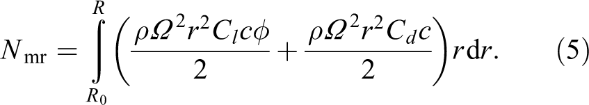
with C _d ≈ C _d0 + C _d1 α + C _d2 α ₂, C _l = aα, and ϕ = ν ₁/(Ωr), where Ω is the velocity of the main rotor, ϕ is the angle of attack of the blade element, c is the inflow angle, α is the chord of the blade, r is the velocity of the radial distance, a is the slope of the lift curve, ρ is the density of the air, and ν1 is the induced speed. Equation (5) can be determined as follows

$\begin{array}{c}{N}_{\text{mr}}=\frac{1}{8}{C}_{d2}\rho c{\Omega }^2\left(R^4-R_0^4\right){\theta }_{\text{mr}}^2+[8C_{d2}\Omega \sqrt{\rho \pi R^2\left(2C_1{\theta }_{\text{mr}}+C_2^2-C_2\sqrt{C_2^2+4C_2{\theta }_{\text{mr}}}\right)}\left(R_0^3-R^3\right)\\ + 4a\Omega \sqrt{\rho \pi R^2\left(2C_1{\theta }_{\text{mr}}+C_2^2-C_2\sqrt{C_2^2+4C_1{\theta }_{\text{mr}}}\right)}\left(R^3-R_0^3\right)+6C_{d2}{C}_1\left(R^2-R_0^2\right)\\ + 6a{C}_1\left(R_0^2-R^2\right)+6C_{d1}\rho \pi \hspace{0.17em}{\Omega }^2{R}^2\left(R^4-R_0^4\right)]\frac{c{\theta }_{mr}}{48\pi R^2}[3C_{d2}{C}_2\sqrt{C_2^2+4C_1{\theta }_{\text{mr}}}\left(R_0^2-R^2\right)\\ + 3a{C}_2\sqrt{C_2^2+4C_1\theta }\left(R^2-R_0^2\right)+4C_{d1}\Omega \sqrt{\rho \pi R^2\left(2C_1{\theta }_{\text{mr}}+C_2^2-C_2\sqrt{C_2^2+4C_1{\theta }_{\text{mr}}}\right)}\left(R_0^3-R^3\right)\\ + 6C_{d0}\rho \pi \hspace{0.17em}{\Omega }^2{R}^2\left(R^4-R_0^4\right)+3a{C}_2^2\left(R_0^2-R^2\right)+3C_{d2}{C}_2^2\left(R^2-R_0^2\right)]\frac{c}{48\pi R^2}\end{array}$

6

where $C_1=\frac{1}{6}\rho abc{\Omega }^2\left(R^3-R_0^3\right)$ ; $C_2=\frac{1}{8}\rho abc\Omega \sqrt{2/\rho \pi R^2}(R^2-R_0^3)$ ; and b, R, and θ _mr are the number and radial of the rotor and pitch angle of the main rotor, respectively. The force is produced by the tail rotor as follows

$F_{\text{tr}}=\frac{1}{2}\rho a_{\text{tr}}{b}_{\text{tr}}{c}_{\text{tr}}{\Omega }_{\text{tr}}^2{\displaystyle \underset{R_{\text{tr}0}}{\overset{R_{\text{tr}}}{\int }}\left({\theta }_{tr}{r}_{tr}^2-\frac{{\upsilon }_{tr1}}{\Omega }r\right)}\hspace{0.17em}\text{d}{r}_{\text{tr}}$

7

${\upsilon }_{\text{tr1}}=\sqrt{\frac{T_{\text{tr}}}{2\rho A_{\text{tr}}}}$

8

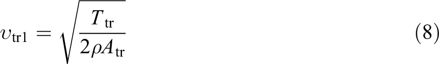
By substituting equation (8) into equation (7), we obtain the following

$F_{\text{tr}}=\frac{1}{2}\rho a_{\text{tr}}{b}_{\text{tr}}{c}_{\text{tr}}{\Omega }_{\text{tr}}^2{\displaystyle \underset{R_{\text{tr0}}}{\overset{R_{\text{tr}}}{\int }}\left({\theta }_{\text{tr}}{r}_{\text{tr}}^2-\sqrt{\frac{T_{\text{tr}}}{2\rho A_{\text{tr}}}}\frac{r}{{\Omega }_{\text{tr}}}\right)}\hspace{0.17em}\text{d}{r}_{\text{tr}}=C_3{\theta }_{\text{tr}}+\frac{1}{2}{C}_4(C_4+\sqrt{C_4^2+4C_3{\theta }_{tr}}$

9

where $C_3=\frac{1}{6}\rho a_{\text{tr}}{b}_{\text{tr}}{c}_{\text{tr}}{\Omega }_{\text{tr}}^2\left(R_{\text{tr}}^3-R_{\text{tr0}}^3\right)$ , $C_4=\frac{1}{8}\rho a_{\text{tr}}{b}_{\text{tr}}{c}_{\text{tr}}{\Omega }_{\text{tr}}\sqrt{2/\rho \pi R_{\text{tr}}^2}\left(R_{\text{tr}}^2-R_{\text{tr0}}^2\right)$ , a _tr is the slope of the lift curve, b _tr is the number of rotors, c _tr is the chord of the blade, ν _tr is the induced velocity of the tail rotor, r _tr is the radial distance, θ _tr is the pitch angle, Ω _tr is the velocity of the tail rotor, and A _tr is the area of the tail rotor disk. The force produced by the main rotor is computed as follows

$F_{\text{mr}}=C_1{\theta }_{\text{mr}}+\frac{1}{2}{C}_2\left(C_2+\sqrt{C_2^2+4C_1{\theta }_{\text{mr}}}\right)$

10

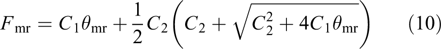
Equations (6) and (10) show that the tail rotor thrust F _tr and main rotor torque N _mr maintains a coupling relationship. Simultaneously, these nonlinear equations are complicated. Therefore, designing the controller is difficult. A simplified equation is thus used as follows

$N_{\text{mr}}=c_{N2}{\theta }_{\text{mr}}^2+c_{N1}{\theta }_{\text{mr}}+c_{N0}$

11

where $c_{N2}$ , $c_{N1}$ , and $c_{N0}$ are determined by the speed of the main rotor and the shape of the blades. Similarly, the lift of the tail rotor is approximated as follows

$F_{\text{tr}}=c_{F2}{\theta }_{\text{tr}}^2+c_{F1}{\theta }_{\text{tr}}+c_{F0}$

12

where $c_{F2}$ , $c_{F1}$ , and $c_{F0}$ are determined by the velocity of the tail rotor and shape of the blades. Equations (3), (4), (11), and (12) are combined, and the non-affine is used to design the controller as follows

$I_{zz}\dot{\gamma }=z_{1r}+z_2\theta -\left(c_{N2}{\theta }_{\text{mr}}^2+c_{N1}{\theta }_{\text{mr}}+c_{N0}\right)+\left(c_{F2}{\theta }_{\text{tr}}^2+c_{F1}{\theta }_{\text{tr}}+c_{F0}\right)l_{\text{tr}}$

13

where z ₁ and z ₂ are the damping constants. Equation (13) expresses the coupled relationship between the tail rotor force and the main rotor torque. This equation is nonlinear in the control input, which contains two-order time variants. Designing a controller for a system with non-affine nonlinear control input is extremely complicated. Based on the proposed yaw dynamic ²⁹

$\dot{\theta }=\gamma$

14

$\dot{\gamma }=a_1\gamma +a_2\theta +b_1{\delta }_{ped}+b_2{\delta }_{ped}^2$

15

where a ₁, a ₂, b ₁, and b ₂ are the unknown parameters. Assuming x ₁ and x ₂ correspond to θ, γ, respectively, u denotes a tail rotor collective input, g denotes a vector [b ₁, b ₂]. The equations (14) and (15) can be presented as

$\begin{array}{c}{\dot{x}}_1=x_2\\ {\dot{x}}_2=f\left(x\right)+gu\\ y=x_1\end{array}$

16

where ${\left[x_1,x_2\right]}^{\text{T}}$ is the state vector, y the system output, u the control input signal. The equation (16) can be considered a second-order system. The unknown parameters will be estimated in the “System Identification” section.

System identification

LM method

The nonlinear least-squares method estimates the parameter, which was described in detail in previous studies. ^{30 –33} LM has been considered as the combination of the steepest algorithm and the Gauss–Newton algorithm. During operation, LM switches between these two algorithms. The update rule of LM can be briefed as

$\widehat{x}\left(k+1\right)=\widehat{x}\left(k\right)-{\left[J_k^T{J}_k+\mu I\right]}^{-1}{J}_k{e}_k$

17

where J is the Jacobian matrix; μ, the combination coefficient, is always positive; I is the identity matrix; e is the error; and the value of combination coefficient, μ, is the condition for switching. Specifically, if μ is very small (nearly zero). The Gauss–Newton method is used. Otherwise, if value of μ is large. The steepest descent method is used. LM has been realized and integrated as function in MATLAB. Hence, it is available to use for identification work. The procedure of system identification will be introduced in the next section.

System identification procedure

The helicopter used is a Raptor 30v2 in X-Plane simulator. To collect estimated data, software-in-the-loop (SIL) is constructed based on the Simulink and X-Plane simulation environments. Four PID controllers developed in Simulink send commands to the X-Plane to maintain the operations of the helicopter at trim condition as shown in Figure 1. Simultaneously, the flight data are sent from X-Plane to Simulink via user datagram protocol (UDP). Given that the helicopter is at the trim condition, the maneuver (Figure 2) is sent to the cyclic pedal input. A total of 10 eligible data sets are stored to estimate the process. The identity of the yaw motion is performed through the LM method, following the sequence of the flowchart shown in Figure 3. The last step in the system identification procedure is validation. This step decides which estimated model is the best by comparing the response of the actual system with that of the predicted model. The quality of the expected result is calculated in percentage by the variance accounted for, as shown in equation (18), where i = 1, 2, 3,…N, and N is the total number of data. x_i is the measured value, and ${\widehat{x}}_i$ is the predicted value. A value of 100% indicates that the output of the predicted model fits the measured output completely.

$\text{VAF}=\text{max}\left\{1-\Vert \frac{\text{var}(x_i-{\widehat{x}}_i)}{\text{var}(x_i)}\Vert ,0\right\}\times 100\%$

18

Figure 1.

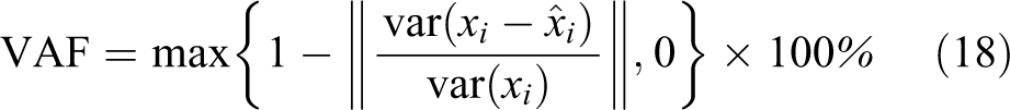
Diagram of the SIL for collecting flight data from X-Plane®.

Figure 2.

Maneuver for collecting yaw flight data motion.

Figure 3.

Flowchart of the estimated procedure. LM: Levenberg–Marquardt.

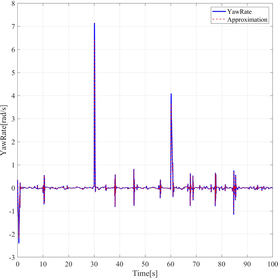
The best result of the system identification is shown in Figure 4. The output of the predicted model agrees with the measured value. The estimated values are shown in the Table 1.

Figure 4.

Result of the yaw motion identification.

Table 1.

The predicted values.

Parameters	a1	a2	b1	b2
Estimated value	1	0	−10.05	0

Adaptive control of a discrete-time system

In this section, a direct adaptive control is presented. The adaptation laws based on the discrete-time Lyapunov stability theory ensures a stable closed-loop tracking control. The augmented error approach provides a suitable way to derive adaptation and control law for uncertain system and guarantee global stability. More details about this approach are presented in the studies. ^34,35

The adaptation law

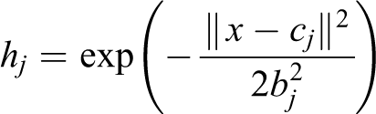
The structure of the radial basis function (RBF) neural network is shown in Figure 5. Where $x={\left[x_1{x}_2\dots x_n\right]}^{\text{T}}$ is the input vector. $h={\left[h_1{h}_2\dots h_n\right]}^{\text{T}}$ is the hidden layer. And h_i is the Gaussian function value for neural network j in the hidden layer.

$h_j=\text{exp}\left(-\frac{\parallel x-c_j\parallel {}^2}{2b_j^2}\right)$

19

where $c=\left[c_{ij}\right]=\left[\begin{array}{ccc}{c}_{11}& \dots & c_{1m}\\ \dots & \dots & \dots \\ c_{n1}& \dots & c_{nm}\end{array}\right]$ is the coordinate value of the center point of the Gaussian function of neural network j. $b=\lceil {\begin{array}{ccc}{b}_1& \dots & b_m\end{array}\rceil }^{\text{T}}$ expresses the width value of the Gaussian function for neural network j. $w={\begin{array}{ccc}\lceil w_1& \dots & w_m\rceil \end{array}}^{\text{T}}$ is the weight value of the RBF. The output of the RBF neural network is calculated by equation (20).

$f=w^{\text{T}}h=w_1{h}_1+w_2{h}_2+\dots +w_n{h}_n$

20

Figure 5.

RBF neural network structure.

Based on the system identification results, the yaw dynamic can be written as

$y\left(k+1\right)=f\left[x\left(k\right)\right]+u\left(k\right)$

21

where x(k) is the state vector, u(k) the control input, and y(k) the plant output. The designed controller gives good tracking performance applied to the plant in equation (21). Define $\widehat{f}\left[x\left(k\right)\right]$ as the approximation of f[x(k)], it is determined in equation (22) as

$\widehat{f}\left[x\left(k\right),\widehat{w}\left(k\right)\right]=\widehat{w}{\left(k\right)}^{\text{T}}h\left[x\left(k\right)\right]$

22

where $\widehat{w}\left(k\right)$ is the estimation value of $w\left(k\right)$ . Assuming that ${\epsilon }_f$ is the arbitrary non-zero approximation error bound. The optimal basis function parameters and output layer parameters $\widehat{w}=w^{\text{*}}$ always exist. It leads to the network that satisfies the following condition

$|\Delta f\left(x\right)|\le {\epsilon }_f$

23

where

$\Delta f\left(x\right)=\widehat{f}\left(x,w^{\text{*}}\right)-f\left(x\right)$

24

$\Delta f\left(x\right)$ is the optimal network approximation error. It is observed that $\widehat{w}\left(k\right)$ is recursively adjusted via the online adaptive law, which guarantees system stability and convergence of tracking error. Define the general network approximation error following

$\overline{f}\left[x\left(k\right)\right]=f\left[x\left(k\right)\right]-\widehat{f}\left[x\left(k\right),\widehat{w}\left(k\right)\right]$

25

Substituting equations (22) and (24) into equation (25) gives

$\overline{f}\left(x\left(k\right)\right)=-\overline{w}{\left(k\right)}^{\text{T}}h\left(x\left(k\right)\right)-\Delta f\left(x\left(k\right)\right)$

26

where $\overline{w}\left(k\right)=\widehat{w}\left(k\right)-w^{\text{*}}$ denotes the parameter error. The tracking error is determined as $e\left(k\right)=y\left(k\right)-y_d\left(k\right)$ , with $y_d\left(k\right)$ as reference. Assuming that e(k) asymptotically converges to zero from any initial condition, if it satisfies the following equation

$e\left(k+1\right)+c_{1}e\left(k\right)=0$

27

The control signal is calculated following the adaptive law

$u\left(k\right)=y_d\left(k+1\right)-\widehat{f}\left[x\left(k\right),\widehat{w}\left(k\right)\right]-c_{1}e\left(k\right)$

28

where $|c_1|<1$ , and $\widehat{f}(.)$ is the approximation of $f\left(x\right)$ . It is observed that the control law includes tracking error e(k) and the network approximation error $\overline{f}\left[x\left(k-1\right)\right]$ . It is considered as the derivation of stable adaptation law by Lyapunov techniques. Substitute equations (25) and (28) into equation (21), we obtain the error dynamic equation as

$e\left(k\right)+c_{1}e\left(k-1\right)=\overline{f}\left[x\left(k-1\right)\right]$

29

Note that, in equation (26), the nonzero inherent network approximation error $\Delta f(.)$ directly affects the above error dynamic equation via the term $\overline{f}(.)$ , where it effectively appears as an additive disturbance term. The error dynamic equation can be equivalently presented in the following transfer function form

$e\left(k\right)={\Gamma }^{-1}\left(z^{-1}\right)\left[\overline{f}(x\left(k-1\right))\right]$

30

where $\Gamma \left(z^{-1}\right)=1+c_1{z}^{-1}$ , and $z^{-1}$ denotes the discrete-time delay operator. In order to keep the stability of the derivative adaptation laws, the augmented error is proposed in the following form

$e_1\left(k\right)=\beta (e\left(k\right)-{\Gamma }^{-1}\left(z^{-1}\right)\left[v\left(k\right)\right])$

31

where β is a positive, nonzero constant. Substituting equation (31) into (29)

$e_1\left(k\right)={\beta \Gamma }^{-1}\left(z^{-1}\right)\left[\overline{f}(x\left(k-1\right))-v\left(k\right)\right]$

32

which leads to the time-domain relation

$e_1\left(k-1\right)=\frac{\beta (\overline{f}(x\left(k-1\right))-v\left(k\right))-e_1\left(k\right)}{c_1}$

33

The auxiliary signal v(k) will be determined subsequently, as part of the design procedure. And the augmented error signal $e_1\left(k\right)$ is utilized to control the adaptation law.

$\Delta \widehat{w}\left(k\right)=\{\begin{array}{c}\frac{1}{\gamma c_1^2}h\left(x\left(k-1\right)\right)e_1\left(k\right)\text{ if }|e_1\left(k\right)|>{\epsilon }_f/G\\ \mathrm{\hspace{1em}\hspace{1em}\hspace{1em}\hspace{1em}0}\text{\hspace{1em}\hspace{1em}\hspace{1em}\hspace{1em} if }|e_1\left(k\right)|\le {\epsilon }_f/G\end{array}$

34

where $\Delta \widehat{w}\left(k\right)=\widehat{w}\left(k\right)-\widehat{w}\left(k-1\right)$ , γ and G are strictly positive constants, and c ₁ is a nonzero constant with $|c_1|<1$ .

Stability analysis

Considering the discrete-time Lyapunov function as

$V\left(k\right)=e_1^2\left(k\right)+\gamma {\overline{w}}^{\text{T}}\left(k\right)\overline{w}\left(k\right)$

35

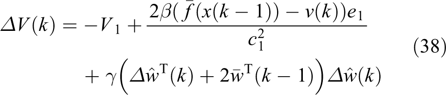
The first difference

$\Delta V\left(k\right)=V\left(k\right)-V\left(k-1\right)$

36

$\Delta V\left(k\right)=e_1^2\left(k\right)-e_1^2\left(k-1\right)+\gamma \left({\overline{w}}^{\text{T}}\left(k\right)+{\overline{w}}^{\text{T}}\left(k-1\right)\right)(\overline{w}\left(k\right)-\overline{w}\left(k-1\right))$

37

Substituting equation (31) into equation (35)

$\Delta V\left(k\right)=-V_1+\frac{2\beta (\overline{f}(x\left(k-1\right))-v\left(k\right))e_1}{c_1^2}+\gamma \left(\Delta {\widehat{w}}^{\text{T}}\left(k\right)+2{\overline{w}}^{\text{T}}\left(k-1\right)\right)\Delta \widehat{w}\left(k\right)$

38

where

$V_1=\left[\frac{e_1^2\left(k\right)\left(1-c_1^2\right)}{c_1^2}+\frac{{\beta }^2(\overline{f}{\left(x\left(k-1\right)-v{\left(k\right)}^2\right)}^2}{c_1^2}\right]\ge 0$

39

Since $0<c_1^2<1$ , and the substitution of equation (26) into (38)

$\Delta V\left(k\right)=-V_1+2{\overline{w}}^{\text{T}}\left(k-1\right)\left[\gamma \Delta \widehat{w}\left(k\right)-\frac{\beta }{c_1^2}h\left(x\left(k-1\right)\right)e_1\left(k\right)\right]-\frac{2\beta }{c_1^2}\left[\Delta f(x\left(k-1\right))+v\left(k\right)\right]e_1\left(k\right)+\gamma \Delta {\widehat{w}}^{\text{T}}\left(k\right)\Delta \widehat{w}\left(k\right)$

40

Substituting equation (32) into equation (36)

If $|e_1\left(k\right)|>{\epsilon }_f/G$

$\Delta V\left(k\right)=-V_1-\frac{2\beta }{c_1^2}\left[\Delta f(x\left(k-1\right))+v\left(k\right)\right]e_1\left(k\right)+{\left(\frac{\beta }{\sqrt{\gamma }{c}_1^2}\right)}^2{h}^{\text{T}}(x\left(k-1\right))h(x\left(k-1\right))e_1^2$

41

If $|e_1\left(k\right)|>{\epsilon }_f/G$

$\Delta V\left(k\right)=-V_1-\frac{2\beta }{c_1^2}\left[{\overline{w}}^{\text{T}}\left(k-1\right)h(x\left(k-1\right))+v\left(k\right)+\Delta f(x\left(k-1\right))\right]e_1\left(k\right)$

42

The aim is that $\Delta V\left(k\right)$ is negative. Therefore, the auxiliary signal v(k) has to be designed so that $e_1\left(k\right)\to 0$ could deduce $e\left(k\right)\to 0$ . Choosing the auxiliary as

$v\left(k\right)=v_1\left(k\right)+v_2\left(k\right)$

43

where

$v_1\left(k\right)=\frac{\beta }{2\gamma c_1^2}{h}^{\text{T}}(x\left(k-1\right))h(x\left(k-1\right))e_1\left(k\right)$

44

$v_2\left(k\right)=G{e}_1\left(k\right)$

Substituting $v\left(k\right)$ in the equation (39), corresponding to $|e_1\left(k\right)|>{\epsilon }_f/G$

$\Delta V\left(k\right)<\frac{-2\beta }{c_1^2}\left[\Delta f(x\left(k-1\right))+G{e}_1\left(k\right)\right]e_1\left(k\right)$

45

Because $|\Delta f\left(x\right)|\le {\epsilon }_f$ by definition, hence, under the condition $|e_1\left(k\right)|>{\epsilon }_f/G$

$e_1\left(k\right)>\frac{|\Delta f(x\left(k-1\right))|}{G}$

46

and

$e_1^2\left(k\right)>\frac{|\Delta f(x\left(k-1\right))e_1\left(k\right)|}{G}\ge \frac{-\Delta f(x\left(k-1\right))e_1\left(k\right)}{G}$

47

Then,

$\left[\Delta f(x\left(k-1\right))+G{e}_1\left(k\right)\right]e_1\left(k\right)>0$

48

Then $\Delta V\left(k\right)<0$ , and if $|e_1\left(k\right)|\le {\epsilon }_f/G$ , tracking performance is satisfied. $\Delta V\left(k\right)$ can take on any value, either positive or negative.

Algorithm of the design system

As presented in the yaw dynamic section, the yaw dynamic is the second-order system, where state vector as yaw angle (ψ) and yaw rate (r). And the relationship between these variables is presented following equation $\dot{\psi }=r$ . On the other hand, the system identification results showed that yaw rate has an important role in yaw dynamic. Moreover, the yaw and heave motions are considered as the coupled dynamic. ¹ So, the designed controller is developed based on yaw rate approximation, tracking error e(k), and main rotor collective input by the Lyapunov techniques.

Assuming y_d as the target value

$y_d={\left[\begin{array}{cc}{\psi }_{\text{Ref}.}& {\dot{\psi }}_{\text{Ref}.}\end{array}\right]}^{\text{T}}$

49

Defining y as the state feedback value

$y={\left[\begin{array}{cc}\psi & r\end{array}\right]}^{\text{T}}$

50

Defining E as the tracking error

$E=y_d-y={\left[\begin{array}{cc}{e}_{\psi }& -r\end{array}\right]}^{\text{T}}$

51

where ${\psi }_{\text{Ref}.}$ is the constant. Its derivative is zero. So, the tracking error E has the form as in equation (51).

Based on the Lyapunov techniques, the proposed control law is as following

$u=\frac{1}{b_1}\left[-\widehat{f}(x\left(k\right))+K^{\text{T}}E\right]+{\delta }_{\text{col}}$

52

where $\widehat{w}\left(k\right)$ is updated following the adaptive law

$\begin{array}{l}\widehat{w}\left(k\right)=\widehat{w}\left(k-1\right)+\frac{1}{\gamma c_1^2}h(x\left(k-1\right))e_1\left(k\right)\text{ if }|e_1\left(k\right)|>{\epsilon }_f/G\\ \hspace{1em}\hspace{1em}\hspace{1em}\hspace{1em}\widehat{w}\left(k\right)=\widehat{w}\left(k-1\right)\text{\hspace{1em}\hspace{1em}\hspace{1em}\hspace{1em}\hspace{1em} if }|e_1\left(k\right)|\le {\epsilon }_f/G\end{array}$

53

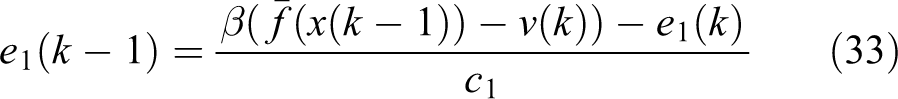
in which, e ₁(k) is the augmented error

$e_1\left(k\right)=\frac{-c_1{e}_1\left(k-1\right)+\beta (e\left(k\right)+c_{1}e\left(k-1\right))}{1+\beta ({v^{\prime }}_1\left(k\right)+G)}$

54

${v\prime }_1\left(k\right)=\frac{\beta }{2\gamma c_1^2}{h}^{\text{T}}(x\left(k-1\right))h(x\left(k-1\right))$

55

where $\widehat{w}$ is the estimated parameter for w, $\widehat{f}(x\left(k\right))$ is the approximated function of f(x(k)), γ, c ₁, ε_f , and G are the constants, which are defined by the user. Notice that |c ₁| < 1, γ, and G are strictly positive constants. Based on the proposed control law, the entire design system is described in Figures (6) to (8).

The diagram of the control scheme of adaptive radial basis function neural network (ARBFNN) follows

Figure 6 is the structure of the developed system. The role of the measurement block is to collect the flight data. The controller block uses three PID controllers to manage pitch, roll, and vertical motion. Yaw motion is controlled by the current method. Its structure is illustrated in Figures 7 and 8. It involves a controller, which is designed based on an adaptive RBF neural network algorithm and the yaw dynamic. The controller processes and generates the commands, lateral (Lat), longitudinal (Lon), collective (col), and pedal (Ped) cyclic, corresponding to the desired and feedback signals. These commands are sent to X-plane via UDP protocol. The algorithm of the adaptive controller is expressed in the following steps:

Step 1: Initial values: c ₁, β, γ, ε_f , G, W, c, b, E, K

Step 2: Calculate the output of the hidden layer; equation (19) is as follows

$h_j=\text{exp}\left(-\frac{\parallel x-c_j{\parallel }^2}{2b_j^2}\right)$

• Step 3: Calculate the augmented error; equations (54) and (55) is as follows

$e_1\left(k\right)=\frac{-c_1{e}_1\left(k-1\right)+\beta (e\left(k\right)+c_{1}e\left(k-1\right))}{1+\beta ({v^{\prime }}_1\left(k\right)+G)}$

${v\prime }_1\left(k\right)=\frac{\beta }{2\gamma c_1^2}{h}^{\text{T}}(x\left(k-1\right))h(x\left(k-1\right))$

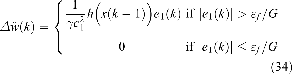
• Step 4: Update neural network weights; equation (53) is as follows

$\widehat{w}\left(k\right)=\widehat{w}\left(k-1\right)+\frac{1}{\gamma c_1^2}h(x\left(k-1\right))e_1\left(k\right)\text{ if }|e_1\left(k\right)|>{\epsilon }_f/G$

$\widehat{w}\left(k\right)=\widehat{w}\left(k-1\right)\text{ \hspace{1em}\hspace{1em}\hspace{1em}\hspace{1em}\hspace{1em}\hspace{1em}\hspace{1em}\hspace{1em}\hspace{1em} if }|e_1\left(k\right)|\le {\epsilon }_f/G$

• Step 5: Calculate the approximation function; equation (22) is as follows

$\widehat{f}(x\left(k\right))=\widehat{w}{\left(k\right)}^{\text{T}}h(x\left(k\right))$

• Step 6: Calculate the output control signal; equation (52) is as follows

$u=\frac{1}{b_1}\left[-\widehat{f}(x\left(k\right))+K^{\text{T}}E\right]+{\delta }_{\text{col}}$

Figure 6.

Diagram of the system.

Figure 7.

Control scheme of the developed system.

Figure 8.

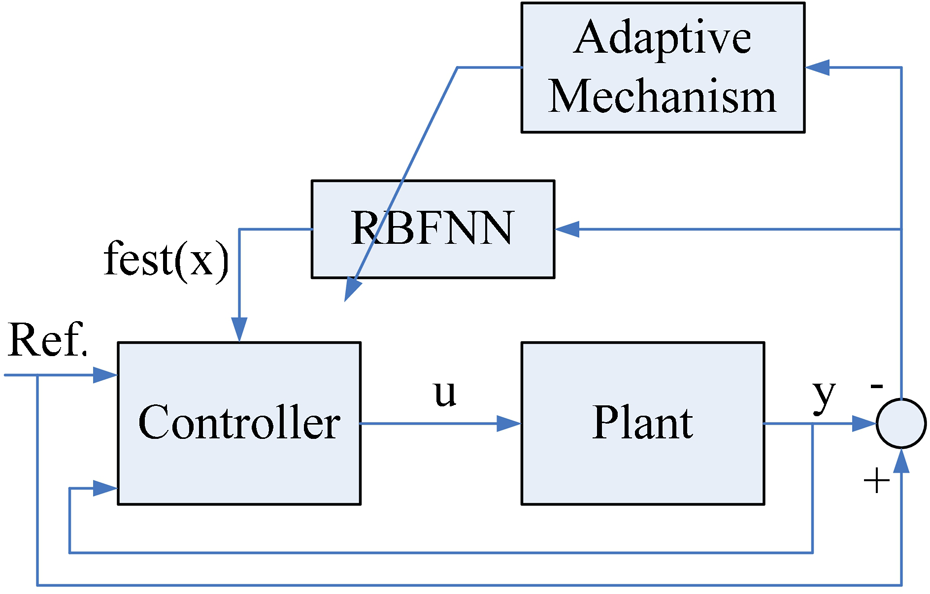
Block diagram of the closed-loop neural-based adaptive control scheme.

In this article, the initial values are defined following

$c_1=0.07;\hspace{0.17em}\beta =0.001;\hspace{0.17em}\gamma =0.001;\hspace{0.17em}{\epsilon }_f=0.003;\hspace{0.17em}G=5000;\hspace{0.17em}b=2$

$W={\left[-12,-9,-6,-3,0,3,6,9,12\right]}^{\text{T}}$

$c=\left[-15,-11.25,-7.5,-3.75,0,3.75,7.5,11.25,15\right]$

$K={\left[15,50\right]}^{\text{T}}$

Simulation results and discussions

The simulation is performed in two cases: ideal and turbulent environments, which are set up in X-Plane simulator as shown in Figures 14 (a) and 14 (b), respectively. The simulation results are shown in Figures 9 to 13. In the ideal condition, the fuzzy and the proposed method maintain an effective yaw angle that captures the target value. However, the adaptive RBF neural network controller provides better quality. The current method rapidly reaches the target value, fuzzy results in the slower response, as shown in Figures 9 and 11. The peak values in Figures 11 and 12 are caused by the slower response of the system in comparison with the changes of the target values. Similarly, in the turbulent condition, although the oscillation appears in both controllers, as shown in Figures 10 and 12, the current method still maintains effective yaw angle agreement with the desired value. The curve of fuzzy has a prominent oscillation. Despite, fuzzy rapidly reaches the desired value. The reason, that is, the characteristic of the helicopter is changed dramatically in the wide range, apart from the random disturbance effect. Fuzzy is well-known as a good solution to the nonlinear system. But determining the rule table to achieve the expected quality is the hard task, especially complex system as the helicopter. On the contrary, the proposed method is designed based on the adaptive solution. The neural network weight is updated online using the Lyapunov approach. So, the stability of the entire system and the convergence of the weight adaptation are guaranteed as shown in Figure 13. Hence, it can work effectively under the random disturbance effect and the large range of change.

Figure 9.

Results of the fuzzy and RBF under ideal environment.

Figure 10.

Results of the fuzzy and RBF under turbulent environment. NN: neural network.

Figure 11.

Error of yaw angle in an ideal condition. NN: neural network.

Figure 12.

Error of yaw angle in a turbulent condition. NN: neural network.

Figure 13.

Yaw rate and approximation value. NN: neural network.

Figure 14.

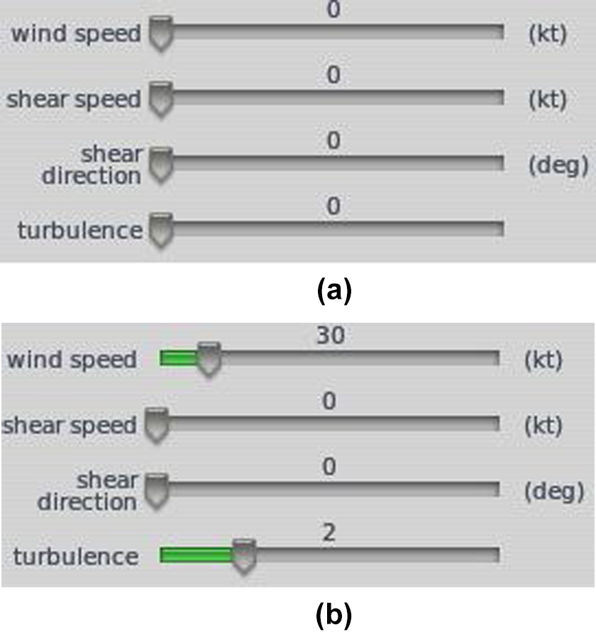
X-Plane® flight conditions (a) Ideal condition; (b) turbulent condition.

Conclusions

This study, the adaptive based on neural approximation has proposed for tracking control of yaw motion. Firstly, the LM method was applied to estimate the affine model of the yaw channel. Then, adaptation and control law are defined based on the Lyapunov and the augmented error approach. Finally, the design system is evaluated under ideal and turbulent environments. Compared with the performance of the fuzzy controller, that of the proposed method is significantly better. The proposed approach has the potential for actual system development. The future works of this study are to develop a fully autonomous flight control system based on the proposed method and to implement the proposed method in real flight tests of small-scale unmanned helicopters.