
Abstract
This article proposes and completely describes a modification of the Hybrid A* method used for navigation of a non-holonomic mobile wheeled robot. Our modification allows straightforward multi-criterial adjustment of the algorithm according to the desired behavior considering not only traveled distance but also time, changing of direction, stopping, going backwards while avoiding obstacles. The obstacle avoidance algorithm evaluates the danger of collision smoothly (not-binarily) using danger fields. Such behavior reflects human-like sensing of danger—the closer to the obstacle the robot is, the higher is the danger of collision. A modified uniform state expansion method has been used to cover the state space of the robot more uniformly providing the possibility of precise near-target navigation. A greed factor has been introduced to decrease the computational time and improve the real-time performance of the algorithm.
Introduction
The navigation of the mobile robot is a dynamic control process during which the control algorithm computes actions which lead the mobile robot to the target. The position of the robot and the target can be defined by three degrees of freedom (3 DoF)—Cartesian coordinates x, y, and direction ψ. The non-holonomic robot has non-zero minimal turning radius
One of the great methods of navigation for wheeled mobile robots is a Vector Field Histogram (VFH) combined with the A* searching algorithm (abbreviated as VFH*). The method was originally proposed by Ulrich and Borenstein.
4
The concept of the method is described by following steps: The current position of the robot is expanded by admissible actions into new projected positions. Each new position is evaluated with respect to (w.r.t.) the target and the previous position. The position that is closer to the target and requires less maneuvering, has a lower cost. If the new position collides with an obstacle, the position is rejected. The total cost of the position is a sum of the previously spent cost and the estimated further cost. Positions are recursively explored up to a given depth or until the target is reached. The A* searching algorithm is used to achieve optimal behavior. Searching is optimal and complete if the estimated cost is always smaller or equal to the true cost. The first action along the found trajectory is physically applied to the robot and the whole process repeats. The navigation is local (does not consider the whole world but only limited surroundings) and real-time.
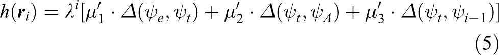
The original paper 4 proposed the following cost function for the first expansion

and for deeper expansions

where i is the depth of the expansion,

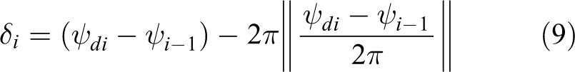
The delta operator over directions is defined by formula

A heuristic estimation of the future cost is
Coefficient
The main drawbacks of the original VFH* algorithm are: The target is defined only by direction (as the target is in infinity) within the method. The original cost function does not consider the distance travelled by the robot. Each state used in prediction is expanded only to different directions, but not to different distances (see Figure 1). Therefore, the state space is not covered uniformly.

Exploration of the nearby robot’s positions.
Other navigational methods are mainly based on grids. Chung and Huang described a navigation algorithm which represents the world as a 2-D grid of occupied or non-occupied cells. The occupancy grid can be obtained simultaneously from the readings of the robots’ sensors. 5 Many different sensors can be used to detect the surrounding obstacles and the robot’s own position (e.g. encoders, ultrasonic sensors, electronic compass, etc.). 6 Szabo 7 described a method for integration of the sensors’ readings by an event representation. The final path obtained by A* searching contains only eight possible directions alongside the grid or diagonally. 8 Daniel et al. introduced the Theta* algorithm that also uses a grid, but applies an any-angle search algorithm, which allows connection of more distant grid vertices by a straight line (line of sight). The obtained trajectory is more smooth and efficient than only 8-directional trajectory. 9 Yap et al. proposed the Block A* method that utilizes a data base of local distances between blocks. The data base contains more than eight nearest blocks; therefore, it is more efficient than A* or Theta*. 10
To overcome the non-holonomic nature of the planned grid trajectories (not smooth), the Stanford University team building robot Junior for DARPA Urban Challenge 11 developed algorithm named Hybrid A*. The algorithm uses continuous states within 4-D state space (two horizontal coordinates, orientation, and direction of motion—forward or reverse). The surroundings of the best node were explored in six defined directions (combinations of forward/backward throttle and left/straight/right steering), which results in six child states. Each child state is assigned to one horizontal grid cell. To improve the efficiency of the expansion, two different heuristic functions have been used to evaluate each state: the first considering non-holonomic nature of the robot and the second considering obstacles. It results in fewer nodes being required to be explored during navigation. The resultant path is smoothed by Conjugate Gradient filtering. 12
Uniform expansion method
Using the original version of VFH*, the local maneuvering of the robot to a nearby target defined by all three coordinates is not working perfectly. One of the reasons is that the expansion uses constant travel distance (the original histogram used in VFH considered only directions). If the target is closer than the expansion distance, the robot will oscillate. The Hybrid A* algorithm is a good starting point in solving the problem.
To cover the state space

where
The exploration of the near positions around the currently best position is done reversely: first, we set the desired position and then we compute the required action to achieve that position. We assume that the robot’s steering control does not need to be continuous (the curvature of the trajectory may change rapidly). The scenario is illustrated in Figure 2, note that direction (angle)

Approaching the nearby position in the ith expansion depth.
The length and the direction of the distance vector


The angle
where

where

If we assume that the vehicle has two control variables: throttle T and steering S, both are within range

where

where ε is the numerical precision of the data type used in the implementation (e.g.
Within one step of the algorithm, it is reasonable to explore up to the maximal achievable distance, which corresponds to full throttle

where

The final direction of the robot after the turn is

If the computed throttle

Reachable positions from the current position within one exploration step.
To speed up the calculation, it is possible to precompute a set of possible actions
Distance between the robot and the obstacle
Evaluation of collisions requires the distance between the robot’s projection into given position

Minimal distance between the robot and the obstacle.
Position of the robot’s origin is shifted from the rectangle’s centrum

Positions of the obstacle’s corners are

where

The distances between the obstacle’s corner and the robot are

Using similar approach, we obtain positions of the robot’s corners
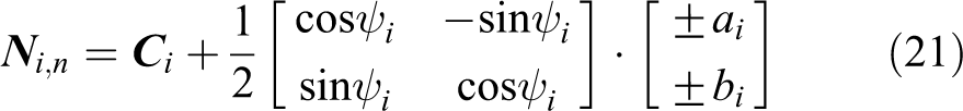
The positions of the robot’s corners w.r.t. the obstacle are

The distances

The distance between the ith robot’s projection and the kth obstacle is the minimum of all eight distances

Clearance
If the obstacle or robot is significantly larger than the grid cell, the proposed method provides significant speedup of the clearance calculation compared to widely used computation of clearance using distances between occupied cells. It also allows more precise maneuvering, since each object may occupy its border cells only partially and the robot and the obstacle may occupy the same cell safely without collision. If the true horizontal footprint of the robot is not rectangular, we use minimal area bounding rectangle.
The reliability and safety of the proposed method depends on the way how the position of the obstacle is obtained. The obstacle may be detected by the robots’ local sensors, or, in case of multiple robots, the information may be provided by communication among them. Then, the most critical factor is the safety of the communication, which has to be evaluated separately. 13
The cost of single exploration step
To find the optimal trajectory, the A* method expands a non-opened node with the smallest (best) total cost during each iteration. The total cost
The cost of distance
The cost of distance is proportional to the length of the trajectory

where
The cost of changing the direction
If it is required to maintain a smooth trajectory, the cost of changing the heading may be introduced. The cost is proportional to the arc angle

where
The cost of stopping the robot
To avoid too many reversal points (point where the vehicle has to stop and change the polarity of throttle), we introduce the cost of stopping

where
The cost of going backwards
For certain mobile robots, it is not convenient to go backwards (e.g. due to worse maneuvering abilities). The cost of going backwards is

where
The cost of danger
The most crucial part of the navigation is avoiding collisions with obstacles. Chen and Zhang
14
proposed a method for estimation of the distance between moving non-holonomic robots. Since the estimation of the position is not absolutely precise, collision detection should not be binary (the real position of the robot could collide with an obstacle while the estimated position does not collide). Therefore, we have introduced a danger field, which is derived from the potential field navigation method. The danger field defines a dimensionless danger of collision as a function of the robot’s position

where
The cost of danger is then

where
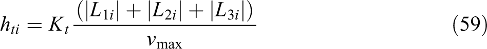
The cost of time
The same trajectory can be achieved by a smaller number of large steps (higher speed) or by a larger number of small steps (small speed). It is desirable to select the faster trajectory, so we have introduced the cost of time. Each time step has the cost proportional to parameter

The overall estimated spent cost is then given by the sum of all partial costs and the cost

Estimation of future cost
In this chapter, we will solve the problem of the minimal distance which has to be run by a non-holonomic wheeled robot to move from one position to another. The space of all possible trajectories is too large to search and contains discontinuities; therefore, it is necessary to choose a certain pattern of the trajectory.
Possible trajectories
We have chosen the trajectory pattern shown in Figure 5 which consists of an initial arc

Trajectory pattern, forward trajectory.
First, we define process variables (we omit the index i of the position
According to Figure 5, the centrum of the initial arc is

analogically, the centrum of the final turn is

The distance vector between the centrum of the turns is then

and its direction is

In the following sections, we will compute all possible trajectories matching the given trajectory pattern.
The same polarity of turns
First, we will discuss the case when both turns have the same polarity

The arc angles are then (according to Figure 5)


Positive sign in indices denotes that the straight segment of the trajectory is traveled forwardly. Polarities

where
There is also a possibility of travelling the straight line reversely (see Figure 6).

The same polarity of turns, reverse trajectory.
The arc angles in the reverse case are


Operation (41) has to be applied to both angles (42) and (43) to keep them within the interval

To denote all possible trajectories in a compact way, we will denote each trajectory as a vector

The opposite polarity of turns
The case when initial and final turns have opposite polarities is shown in Figure 7, the reverse variant is in Figure 8.
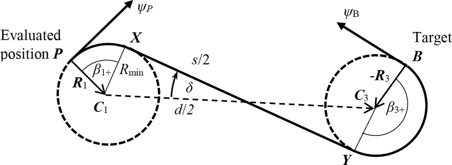
Opposite direction of turns, forward trajectory.
Opposite direction of turns, reverse trajectory.
The arc angles are


where the angle δ (according to the figure) is

The complementary arc angles (dashed arcs) are computed in the same way as in the previous case. From equation (48), it is clear that the trajectory exists only if

The length of the straight section of the trajectory is

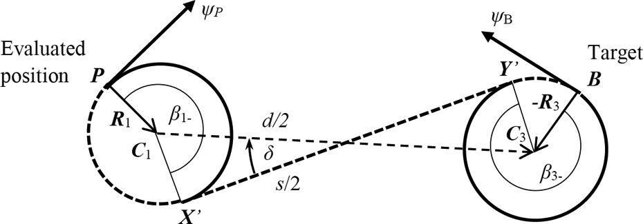
Like in the case when both circles have the same polarity, there is also the possibility to travel reversely (see Figure 8).
The corresponding arc angles are


After removing the period from all arc angles using equation (41), we obtain another set of possible trajectories (valid for the case of opposite arc polarities)

Computing the minimal cost of travelling to the target
There are 4 possible combinations of arc polarities

For each combination, we obtain eight possible trajectories (using equation (45) for the same polarities and equation (53) for the opposite polarities). The full set contains 4 × 8 = 32 possible trajectories matching the defined pattern. Each trajectory has its cost, which reflects the requirements of the application. Generally, the cost increases with the distance, changing of the heading, stopping the robot, or going backwards. Note that we do not evaluate danger (since it must be evaluated at each point of the trajectory). The formulas for predicted future costs are similar to the formulas for the spent cost (equations (25) to (33))


where

The estimated future cost is computed for each of the 32 possible trajectories and the best trajectory is selected.
The greed factor
If the original A* searching algorithm is used, the total cost of any predicted position

The navigation algorithm finds the optimal trajectory but it examines too many nodes which results in poor real-time performance. To speed up the calculation and searching, we have introduced the greed factor γ. It sacrifices a small portion of the optimal (minimal cost) to decrease the number of nodes required to be expanded during search. The modified total cost function replaces equation (61)

When the greed factor is equal to 1, the searching does not consider the spent cost
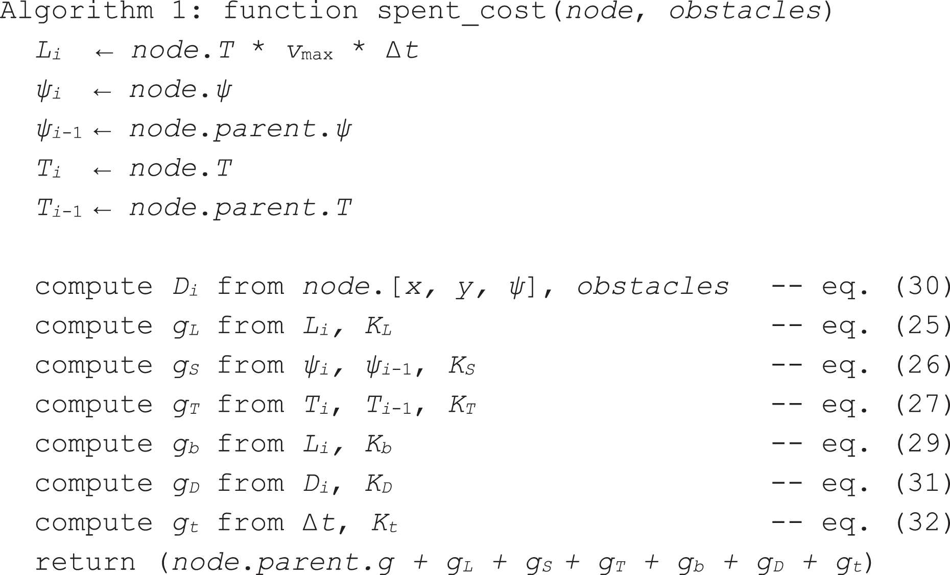
Each predicted state of the robot will be represented by the structure
end
The cost spent from the starting state into predicted state is computed using function
function spent_cost (node, obstacles)

function future_cost (node, target)


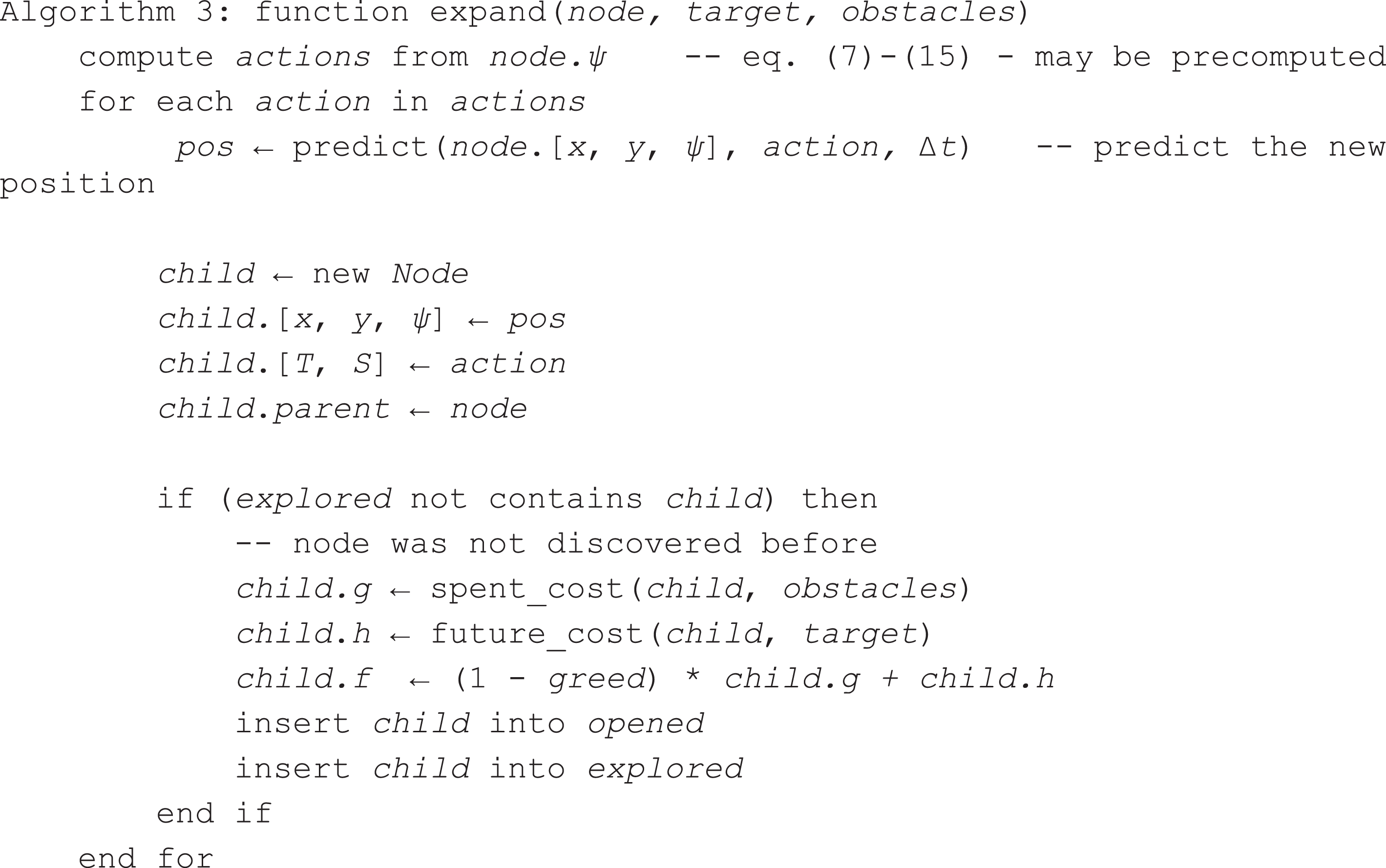
Exploration of the child states is accomplished by the function expand shown in Algorithm 3:
function expand(node, target, obstacles)

Finally, the function navigate implements A* searching with greed factor (see Algorithm 4):
function navigate (from, target, obstacles, T 0 , S 0)


Experimental results
The proposed system has many adjustable parameters. To obtain results, that are comparable across experiments, we have used simulation in the simulated world (see Figure 9). The parameters of the robot were as follows:

The simulated world and the optimal trajectory found (300,260 nodes has been explored).
The world contains 12 static obstacles which makes it difficult for the robot to choose the optimal trajectory (many trajectories have the same cost).
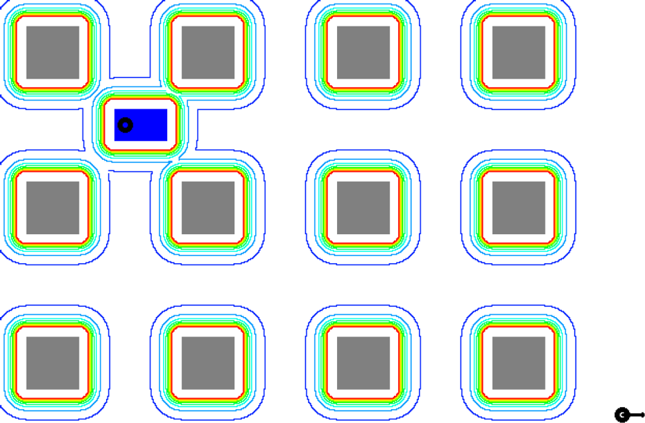
We have evaluated the cost of the found trajectory, the computation time, and the count of explored nodes as a function of the greed factor. All the experiments were conducted with the same pseudorandom set of 1000 targets and 20 different settings of the greed factor (20,000 experiments). The cost constants which describe the properties of the optimal trajectory were set to the following values: the prediction step

Map of danger.
To limit the simulation time, each experiment was limited to 1 s of computational time. If the algorithm did not find the solution within the given time limit, it was considered as unsuccessful. Such targets were removed from the set of targets. The remaining experiments were averaged for the same setting of the greed factor across all targets.
To demonstrate the importance of the uniform expansion method, we compare its performance with the state expansion in six directions only, which was proposed by the original Hybrid A* method.
As predicted, a higher greed factor allows the method to find the trajectory faster but the obtained trajectory is slightly suboptimal (compare Figures 9 and 11). Figure 12 shows the relation between the average cost per one target and the greed factor. With the greed factor from the range of 0 to 0.8, the cost of the trajectory is increasing only slightly (the greed factor
A suboptimal path computed using a greed factor γ = 0.4 (only 49,240 nodes has been explored).

Average cost of the trajectory versus greed factor.
Figure 13 shows the average count of nodes which had to be explored to find the solution. With the greed factor from 0 to 0.3, the average count of nodes decreases almost linearly, and for a greed factor above 0.6, it is almost constant.

Average count of explored nodes versus greed factor.
Computational time is closely related to the count of explored nodes, therefore the relation in Figure 14 is similar to the one in Figure 13. A higher greed factor means lower computational time. For a greed factor above 0.5, the average computational time was below 100 ms.
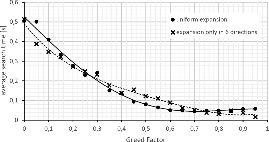
Average computation time versus greed factor.
Since we require the algorithm to operate in real-time, the computation time was limited to 1 s. Figure 15 shows the probability of finding the trajectory within the given time limit. Without the greed factor, solutions for only 20% of the targets were found on time. For a greed factor above 0.5, more than 70% of the solutions were found on time. Note that using only six directions for expansion significantly increases the count of explored nodes, thus finding the solution times out in many cases. Figure 14 shows average of successful searches, therefore, it does not reflect poor probability of finding the solution in case of the six-directional expansion.

Probability of finding the trajectory within timeout (1 s) versus greed factor.
The algorithm has been evaluated in real world using e-puck robot (e-puck is a small mobile robot developed by GCtronic). 17,18 The testing environment with the e-puck robot inside can be seen in Figure 16. The environment has been modeled also in the control program (see Figure 17). The robot accomplished to pass the proposed trajectory while its position has been estimated using onboard odometers.
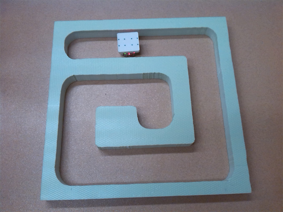
Testing environment with e-puck robot.

Designed trajectory.
Conclusion
Our proposed method improves the evaluation method of the Hybrid A* algorithm. First, we have introduced a uniform state expansion method which improves searching speed and decreases count of nodes needed to be explored. Then, we have modified and simplified the heuristic method used to estimate the future cost required to reach a given target. The navigation algorithm considers not only the length of the trajectory but also reversing, going backwards, changing the direction, the danger of collision, and the time of travel. Each feature is penalized by a separate parameter which allows simple adjustment of the behavior of the algorithm according to the requirements of any application. The evaluation of danger is not binary as used in many implementations of Hybrid A* (e.g. studies by Kurzer 1,19 ), but smooth, which reflects the limited precision of the robot’s localization system.
To speed up the real-time computations, we have used the greed factor which allows us to set the right balance between the required computational power and the cost of the projected trajectory. Our experiments show that a greed factor around 0.5 decreases the cost of the obtained trajectory only by 16% but decreases the computational time 5 times, which greatly improves the real-time performance of the algorithm.
Footnotes
Declaration of conflicting interests
The author(s) declared no potential conflicts of interest with respect to the research, authorship, and/or publication of this article.
Funding
The author(s) disclosed receipt of the following financial support for the research, authorship, and/or publication of this article: This work has been supported by the Educational Grant Agency of the Slovak Republic KEGA, within the projects 014ŽU-4/2018 and 016ŽU-4/2018.