Sage Journals: Discover world-class research

Abstract

There are still some problems need to be solved though there are a lot of achievements in the fields of automatic driving. One of those problems is the difficulty of designing a car-following decision-making system for complex traffic conditions. In recent years, reinforcement learning shows the potential in solving sequential decision optimization problems. In this article, we establish the reward function R of each driver data based on the inverse reinforcement learning algorithm, and r visualization is carried out, and then driving characteristics and following strategies are analyzed. At last, we show the efficiency of the proposed method by simulation in a highway environment.

Keywords

Car-following inverse reinforcement learning (IRL)autonomous vehicle decision-making automatic driving

Introduction

Intelligent driving in intelligent vehicles is a technical high point in industrial technology and is studied by various countries and major technological companies. Car following is one of the most significant and common conditions for manual driving, assisted driving, or unmanned driving.¹ With the rapid growth of urban traffic scale, car following has become the most primary condition encountered by drivers.^2,3 Car-following models have been extensively studied since 1950s,⁴ and the research currently focuses on different fields, such as vehicle engineering, traffic safety, big data and artificial intelligence, psychology, and cognition. Research on car-following behavior gradually extends from the original operation of acceleration, deceleration, and other specific operations to perception, psychology, and physiology. The methodology for studying such behavior has been extended from early mathematic modeling to various fields, such as logistics, planning, transportation, cognitive science, neuroscience, data science, machine learning, and artificial intelligence.^5,6

In 1950, Reuschel studied the car-following behavior of drivers from an operational research perspective,⁷ whereas Pipes proposed the first car-following problem in 1953.^8,9 Existing car-following models (algorithms) can be divided into two categories. The first category is explanatory car-following model. First, the model predetermines some physical quantities in the car-following process to describe the expression using parameters. Then, the unknown parameters of the expression can be determined based on statistics or experience. This type of car-following model often requires assumptions and explanations of the car-following process. The second category is nonexplanatory car-following model. The car-following behavior of drivers is based on a learning algorithm, namely, the fitting or induction of a large number of data.

Explanatory models include linear car-following model, distance inverse model, nonlinear car-following model, memory function model, expected distance model, and physiological–psychological model. In 1958 and 1959, Chandler¹⁰ and Herman^11,12 respectively proposed linear car-following models. In 1959, Gazis et al. presented a range inverse car-following model.¹³ After 2 years, Gazis et al. further proposed a nonlinear car-following model.¹⁴ In 1967, May and Keller completed the fitting of the nonlinear model with actual vehicle data under highway and tunnel conditions.^15,16 In 1993, Ozaki divided driver motion into four stages: acceleration start, deceleration start, acceleration maximum, and deceleration maximum. When separately fitted, the reaction time is strongly dependent on the stage of driving action. In particular, the reaction times are quite different in the acceleration and deceleration stages. Ozaki suggested that the possible reason for this difference is the use of the taillight of a front car during deceleration stages.¹⁷ Lee introduced a memory function model in 1966, in which he thought that drivers responded to the integral of the relative speed of the front vehicle rather than the instantaneous value. He then analyzed its stability. In 1972, Darroch and Rothery used spectral analysis methods. The shape of the memory function was estimated based on the experimental data. They found that Dirac delta function can approximate experimental data; in fact, it corresponds to the linear following model.¹⁸ In 1961, Helly suggested that the driving strategy of drivers not only minimized relative speed but also the difference between real and expected vehicle distances. In 1982, Gabard et al. used Helly’s model in SITRA-B (microscopic traffic flow model).¹⁹ In 1974 and 1988, Weidmann and Leutzbach proposed two unreasonable points of the traditional car-following model: (1) In the previous car-following model, even with a large distance to a front vehicle, testing vehicle will also keep following. (2) The previous car-following model assumed that the drivers had the perfect perception and reaction, even if the external incentive was very small. Therefore, they introduced a perceptual threshold to define the minimum environmental incentive, which can be reacted to by the drivers. Evidently, the perceived threshold increased monotonically with the distance to the car. At the same time, they also found that the perception threshold is different during the acceleration and deceleration phases.²⁰ Explanatory model can generally guarantee the safety of the following process of the car, but accurately describing the highly nonlinear car-following behavior is difficult. Moreover, the model does not have adaptive adjustment ability for different drivers or different conditions.^21,22

With the development of artificial intelligence research, a variety of machine learning methods are the most prominent. These methods have outstanding advantages in dealing with nonlinear problems,^2,7 such as convolutional neural network, reinforcement learning (RL), and inverse reinforcement learning (IRL). A considerable number of researchers have begun to focus on the car-following model based on machine learning methods.^2,7 Richard S Sutton proposed a temporal-difference learning (TD) method.²³ Bradtke and Andrew G Barto established two algorithms which were called least-squares TD (LSTD) and recursive least-squares TD (RLSTD) with the help of the theory of linear least-squares function approximation.²⁴ Michail G Lagoudakis and Ronald Parr proposed an approach called least-squares policy iteration (LSPI) by combining value function approximation with linear architectures and approximate policy. Xu et al. proposed a kernel-based least-squares policy iteration (KLSPI).²⁵ Wei Xia et al. proposed a new control strategy of self-driving vehicles using the deep RL model, in which learning with an experience of professional driver and a Q-learning algorithm with filtered experience replay are proposed.²⁶ Pyeatt and Howe applied RL to learning racing behaviors in Robot Auto Racing Simulator, precursor of the The Open Racing Car Simulator (TORCS) platform.^27,28 Daniele et al. used the tabular Q-learning model to learn the overtaking strategies on TORCS.²⁹ Riedmiller proposed a neural RL method, namely neural fitted Q-iteration (NFQ), to generate control strategy for the pole balancing and mountain car task with least interactions.³⁰ Zheng et al. established a 14-Degree of Freedom (DOF) dynamic model of an autonomous vehicle and use R to build a decision-making system for autonomous driving.³¹ The nonexplanatory model, represented by artificial neural network (ANN), fully demonstrates the high nonlinearity of car-following behavior and has been proven by some researchers to be stable and safe under certain conditions (such as slope input and sinusoidal input). However, the model treats the drivers as a “black box” because such models are not interpretative. Theoretically analyzing whether or not the model is stable or has existing “bad spots” is difficult. Meanwhile, such models are more capable of “cloning” rather than “learning” driving strategies and thus have difficulty in intuitively reflecting “adaptability”. With the change in working conditions and drivers, the change of the model itself is only the weight between nodes, but a direct relationship between the weights and driving behaviors is difficult to establish. As a result, further analysis is also difficult to perform. The lack of flexibility is another major problem with car-following models based on ANNs. A network trained by a data set may not be well applied to another data set. Thus, this present work proposes a learning algorithm with a certain interpretation for car-following model and establishes an anthropomorphic following model. The vital RL and its associated IRL in machine learning provide us a novel idea. Analyzing the car-following behavior of drivers by the following model and proposing the intelligent following algorithm have great value and significance in many fields, such as road safety, driving assistance system, and intelligent driving. The explanatory model is too simple to accurately describe the highly nonlinear car-following behavior and cannot adapt to different drivers and working conditions. Although the nonexplanatory model represented by ANN can fit complicated nonlinear relations, such models are not interpretable. Moreover, the theoretical analysis on the stability or the establishment of the relationship between driving behaviors and neural network structure for further analysis becomes difficult because the drivers are treated as “black box.” Therefore, to implement the anthropomorphic car-following model, the machine learning-based method is used to optimize auto-following algorithm, which is of great value for research. The contribution of this article is briefly described as follows: (1) A learning car-following algorithm with a certain explanation by using IRL combined with the car-following data of driving simulator. (2) The IRL algorithm is designed to learn the reward function R of drivers from driving simulator data. (3) The reward function R of different drivers is visualized under different conditions. (4) The similarities and differences are analyzed, and the IRL algorithm is optimized.

The remaining part of this article is organized as follows: The second part is “Reinforcement learning and inverse reinforcement learning.” The third part is “Design of IRL algorithm.” The fourth part is the “Experiment and analysis” based on the simulation platform and the rest part is “Conclusion and future work.”

Reinforcement learning and inverse reinforcement learning

Reinforcement learning

RL is a vital branch of machine learning, and a typical RL task is usually described by the Markov decision process. The machine (or agent) is in environment E, defining a state space S, where each state is a description of the environment that the agent can perceive. The actions that an agent can perform constitute action space A; $a \in A$ is an action can be taken by an agent. After taking the action, the state transition probability P enables the environment to be transferred from the current state to another state with certain probability. At the same time, as the state transitions, a reward r is the feedback of the environment to the agent according to the potential reward function R.³² A RL task corresponds to the tetrad $E = 〈 S, A, P, R 〉$ ; $P : S \times A \times S \mapsto ℝ$ , which represents the probability of state transition; and $R : S \times A \times S \mapsto ℝ$ , which represents the reward function. As shown in Figure 1, the agent observes state s and then performs action a, s transfers to the next state based on the state transition probability P, and simultaneously an instant reward r is obtained. In RL, agents continuously interact with the environment and update strategies to learn policer $a = π (s)$ .

Figure 1.

Illustration of RL. RL: reinforcement learning.

The relative merits of the strategy depend on the cumulative reward of long-term execution, rather than the instant reward for performing an action. Consequently, the RL task maximizes the long-term cumulative reward generated by the policer. Therefore, this work uses the “γ-discounted cumulative reward” to estimate the long-term cumulative reward, as shown in equation (1)

max_{π} E [\sum_{t = 0}^{+ \infty} γ^{t} r_{t + 1}]

γ is the discount rate, a positive number less than 1, and represents the degree of emphasis that the agent has on future rewards. The greater the value of γ, the more the attention is paid to the future received rewards. r_t is the instant rewards of the tth step, and $E$ is the expression of the expectation of all random variables.

Inverse reinforcement learning

The reward function R plays a crucial role for a deterministic RL task. The setting of R directly determines which strategy the agent will adopt. However, for many RL tasks, the reward function R cannot be predetermined, or the suitable state (strategy) for an agent is unknown. For the car-following decisions studied in this work, different explicit R values for different driver models are difficult to determine, and distinguishing which state (strategy) is good or bad is unclear. Although the relative merits of a strategy are known, specific reward function values are difficult to quantify. IRL is based on a sample data provided by experts, which is reversely introduced as the reword function.³³ The basic idea is to define the strategy with the sample data as π ^* and another strategy as π. The reward function is expressed as a linear function of the state s, that is, $R (s) = ω^{T} s$ . Given the coefficient $ω^{T}$ , ρ represents the cumulative reward, the cumulative reward for the strategy π is shown in equation (2)

ρ (π | ω^{T}) = E [\sum_{t = 0}^{+ \infty} γ^{t} R (s_{t}) | π] = E [\sum_{t = 0}^{+ \infty} γ^{t} ω^{T} s_{t} | π]

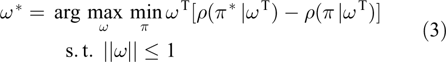
The goal of IRL is to calculate π ^*. When the difference between the optimal and other samples is maximized, some parameters are computed to ensure that the strategy with example data π ^* can be better than any strategy π. The objective function is shown in equation (3)

\begin{array}{l} ω^{*} = arg max_{ω} min_{π} ω^{T} [ρ (π^{*} | ω^{T}) - ρ (π | ω^{T})] \\ s . t . ‖ ω ‖ \leq 1 \end{array}

Design of IRL algorithm

The main purpose of IRL is to obtain the reward function R of drivers. In this work, an IRL algorithm based on the max-margin algorithm is proposed.³⁴ As shown in equations (2) and (3), the algorithm is divided into the following steps:

Determine the state space and implement the transformation of the kernel function.

Obtain the various components $R_{i j}$ for R and calculate the cumulative reward of each component $V_{i j}$ .

Determine the weight of $R_{i j}$ and eventually solve R.

Determine the state space and transform kernel function

The physical quantities that reflect the process of car-following method are as follows: car-following distance d (which is the leading distance between the front vehicle and testing vehicle, and the unit is m), velocity of the testing vehicle v (in unit of $km/h$ ), velocity of front vehicle $v_{front}$ , acceleration of the testing vehicle a, and acceleration of front vehicle $a_{front}$ . For data visualization, this work chooses velocity of the testing vehicle v and car-following distance d to form a 2-D variable as the state space, which constitutes the S in the quadruple $E = 〈 S, A, P, R 〉$ . The 2-D features are transformed by the Gaussian radial kernel function and mapped into the high-dimensional feature space to denote the strong nonlinear relationship in the car-following process. After data preprocessing, the range of the testing vehicle velocity v is limited to $(0, 130 km/h$ ), and the range of the car-following distance d is $(0, 350 m)$ . According to such range of the velocity and distance, velocity v is divided into equal intervals $(v_{1}, v_{2}, \dots v_{15})$ by the interval $9 km/h$ , as shown in equation (4)

v_{i} = 9 (i - 1), 1 \leq i \leq 15

The car-following distance d can be divided into equal intervals, and the interval is $(d_{1}, d_{2}, \dots d_{36})$ , as shown in equation (5)

d_{j} = 9 (j - 1), 1 \leq j \leq 36

Given that the data size of vehicle speed v and distance d is inconsistent, the normalization of all these data is required. The state vector $s = (\frac{25}{9} v, d)$ and kernel vector ${\bar{s}}_{i j} = (\frac{25}{9} v_{i}, d_{j})$ are defined, and the Gaussian radial kernel function is shown in equation (6)

K (S, S_{i, j}) = exp (- \frac{{‖ s - {\bar{s}}_{i, j} ‖}_{2}^{2}}{σ^{2}}), 1 \leq i \leq 15, 1 \leq j \leq 36

If σ ² is selected, then the space expanded by the kernel function can be neither overfitting nor underfitting. After experimental verification, $σ^{2} = 5$ is defined to ensure that the kernel function can obtain a relative equilibrium between underfitting and overfitting.

Calculate reward function and cumulative reward

The requiring reward function R can be written by a linear combination of 540 kernel functions based on the kernel function with state vector, as shown in equation (7)

\begin{array}{l} R (v, d) = \sum_{i = 1}^{15} \sum_{j = 1}^{36} θ_{i, j} R_{i, j} (v, d) = \sum_{i = 1}^{15} \sum_{j = 1}^{36} θ_{i, j} K (s, {\bar{s}}_{i, j}) \\ s = (\frac{25}{9} v, d); {\bar{s}}_{i j} = (\frac{25}{9} v_{i}, d_{j}) \end{array}

Next, the value of each component $R_{i, j} (v, d)$ at each state s of $R (v, d)$ should be calculated, that is, for the action sequence of drivers ${s_{1}, s_{2}, \dots, s_{N}}$ , $R_{i, j} (s_{l}), 1 \leq l \leq N$ is calculated. The solving process is demonstrated in Figure 2.

Figure 2.

Solving process of $R_{i, j} (s_{l})$ .

$R_{i, j} (s)$ is an instant reward, and the cumulative reward $V_{i, j} (s)$ of each state measures the long-term rewards of the state s. Equation (8) shows the calculation of the cumulative reward

V_{i, j} (s_{l}) = \sum_{t = l}^{N} γ^{t - 1} r_{t} = \sum_{t = l}^{N} γ^{t - 1} R_{i, j} (s_{t})

where γ is the discount factor, which evaluates the discount rate of drivers. In this work, the value is selected as $γ = 0.9$ .

Determine the weights of reward function

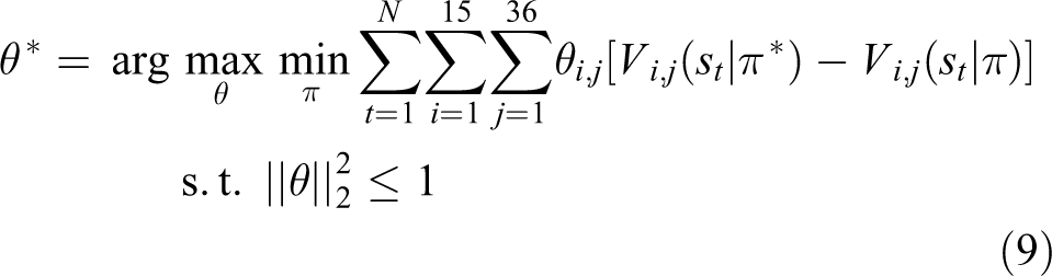
After calculating $R_{i, j} (s)$ , the next step is to determine the parameters $θ_{i, j}$ . Under driving strategy π ^*, the long-term cumulative reward $V (s | π^{*})$ is superior to the rewards under other strategies $V (s | π)$ , as shown in equation (9)

\begin{array}{l} θ^{*} = arg max_{θ} min_{π} \sum_{t = 1}^{N} \sum_{i = 1}^{15} \sum_{j = 1}^{36} θ_{i, j} [V_{i, j} (s_{t} | π^{*}) - V_{i, j} (s_{t} | π)] \\ s . t . {‖ θ ‖}_{2}^{2} \leq 1 \end{array}

where θ is the vector expanded by $θ_{i, j}$ , $s_{t}^{*}$ represents the car-following state sequence under the optimal strategy π ^*, $s_{t}^{(i)}$ represents the car-following state sequence under other strategy, $a_{t}^{*}$ is the action sequence under the optimal strategy π ^*, and $a_{t}^{(i)}$ is the action sequence under other strategies. The corresponding relationship between these variables is shown in Figure 3.

Figure 3.

Relationship between variables of max-margin algorithm based on IRL. IRL: inverse reinforcement learning.

Equation (9) can be transformed into the optimization problem under the inequality constraint, as shown in equation (10)

\begin{array}{l} \sum_{i = 1}^{15} \sum_{j = 1}^{36} θ_{i, j} V_{i, j} (s_{2}^{*}) - \frac{1}{M} \sum_{m = 1}^{M} \sum_{i = 1}^{15} \sum_{j = 1}^{36} θ_{i, j} V_{i, j} (s_{2}^{(m)}) \geq p_{1} \\ \sum_{i = 1}^{15} \sum_{j = 1}^{36} θ_{i, j} V_{i, j} (s_{3}^{*}) - \frac{1}{M} \sum_{m = 1}^{M} \sum_{i = 1}^{15} \sum_{j = 1}^{36} θ_{i, j} V_{i, j} (s_{3}^{(m)}) \geq p_{2} \\ \dots \\ \sum_{i = 1}^{15} \sum_{j = 1}^{36} θ_{i, j} V_{i, j} (s_{N}^{*}) - \frac{1}{M} \sum_{m = 1}^{M} \sum_{i = 1}^{15} \sum_{j = 1}^{36} θ_{i, j} V_{i, j} (s_{N}^{(m)}) \geq p_{N - 1} \\ max_{θ} \sum_{t = 1}^{N - 1} p_{t} \\ s . t . {‖ θ ‖}_{2}^{2} \leq 1 \end{array}

Furthermore, equation (10) can be simplified to equation (11) if only one strategy for each state is present

\begin{array}{l} \sum_{i = 1}^{15} \sum_{j = 1}^{36} θ_{i, j} V_{i, j} (s_{2}^{*}) - \sum_{i = 1}^{15} \sum_{j = 1}^{36} θ_{i, j} V_{i, j} (s_{2}^{(1)}) = p_{1} \\ \sum_{i = 1}^{15} \sum_{j = 1}^{36} θ_{i, j} V_{i, j} (s_{3}^{*}) - \sum_{i = 1}^{15} \sum_{j = 1}^{36} θ_{i, j} V_{i, j} (s_{3}^{(1)}) = p_{2} \\ \dots \\ \sum_{i = 1}^{15} \sum_{j = 1}^{36} θ_{i, j} V_{i, j} (s_{N}^{*}) - \sum_{i = 1}^{15} \sum_{j = 1}^{36} θ_{i, j} V_{i, j} (s_{2}^{(1)}) = p_{N - 1} \\ max_{θ} \sum_{t = 1}^{N - 1} p_{t} \\ s . t . {‖ θ ‖}_{2}^{2} \leq 1 \end{array}

The number of samples is sufficient (for each test, N ≈ 60000); therefore, equation (11) is taken into account in the calculation. For each optimal car-following state, one of the other car-following actions is randomly selected for the solution. The effect of traversing the other strategies for an average performance can be achieved. The selection of the other car-following action is based on the statistics of acceleration of the testing vehicle, which can provide the range of acceleration $[a_{min}, a_{max}]$ . Then, the interval is divided into 10 points as the action set, so other strategies are randomly selected from nine nonoptimal car-following actions. The parameter $θ_{i, j}$ is solved by Lagrange multiplier method or “linprog” function in MATLAB, as shown in equation (12)

θ_{i, j} = \frac{\sum_{2}^{N} [V_{i, j} (s_{t}^{(1)}) - V_{i, j} (s_{t}^{(*)})]}{\sqrt{\sum_{i = 1}^{15} \sum_{j = 1}^{36} {\sum_{2}^{N} [V_{i, j} (s_{t}^{(1)}) - V_{i, j} (s_{t}^{(*)})]}^{2}}}

Experiment and analysis

Experiment setup

Hardware and software

The working conditions of vehicle and the road environment must be precisely controlled to study the car-following behavior of drivers under given conditions. Therefore, this work is based on the dynamic driving simulation test bench of Tsinghua University. The dynamic driving simulation test bench is shown in Figure 4, and its system components are shown in Figure 5.

Figure 4.

Dynamic driving simulation test bench.

Figure 5.

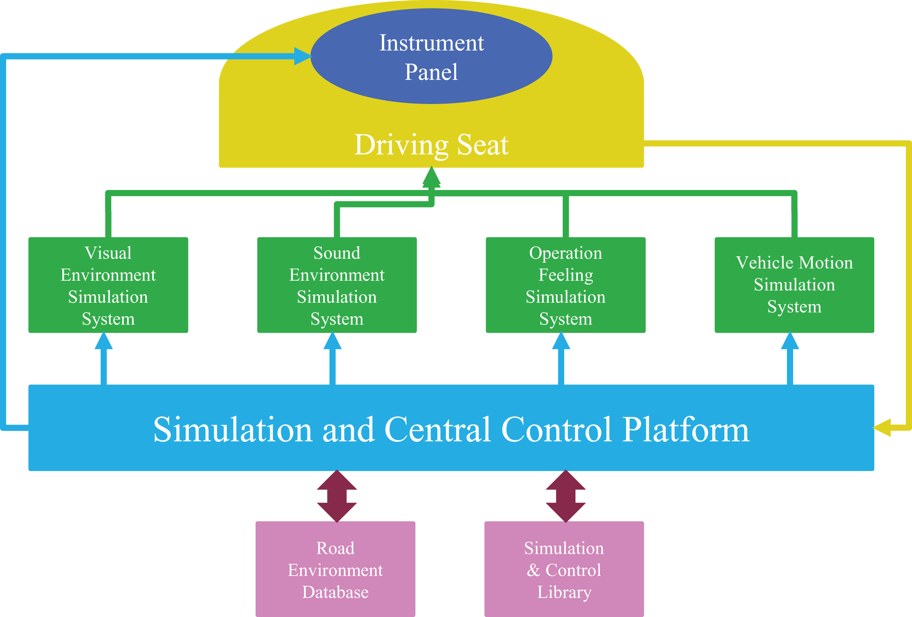
System components of the dynamic driving simulation test bench.

The hardware part of the simulator consists of five parts: simulation cockpit, external visual environment simulation system, vehicle motion simulation system, sound environment simulation system, and operation tactile sensation simulation system.³⁵ The software part of driving simulator consists of six parts: system control module, environment control and scene creation module, simulation calculation module, input and output module, graphics calculation and rendering module, and actuator control module.^36,37

Environment modeling

This work is about the car-following behavior of drivers under a single lane (no lane change, no overtaking, and no traffic light); therefore, the freeway is selected as a road scene. A two-lane road of 200 km in length is designed. The road includes a fast lane, a slow lane, and an emergency lane with widths of 3.75, 3.75, and 2.5 m, respectively. The road model is shown in Figure 6.

Figure 6.

Road model.

Vehicle model

The most common vehicle is chosen as the front car (BMW 3 Series as a template), and the dynamics model of the vehicle was generated by CarSim. In addition, the brake lights turn red when the vehicle is decelerating, which is consistent with the real situation. The road scene of the actual testing process is shown in Figure 7. Three computer screens correspond to three projection screens (middle, left, and right) of the external virtual environment system. These screens constitute the front view of the drivers.

Figure 7.

Road scene of the actual test.

In order to intuitively demonstrate the effectiveness and generalization ability of the IRL algorithm, the experimental data are obtained by selecting two subjects who have been driving for more than 5 years as drivers A and B. According to two different operating conditions of the New European Driving Cycle (NEDC) and Japan’s 10–15, the following experiments are carried out on the driving simulator, the following data of drivers A and B are recorded, and the reward function r of drivers A and B is visualized, giving the NEDC and Japan’s 10–15. For each working condition, two randomly selected tests are performed to verify the reproducibility of the test results.

Experiment result

The entire space $(v, d)$ is traversed, and the test driver’s reward function is shown in Figure 8. The reward information of the drivers can be obtained by analyzing the shape of the reward function surface in Figure 3. A high surface height corresponding to any point on the plane $(v, d)$ indicates great instant reward value at the same point.

Figure 8.

Diagram of the reward function.

The 3-D graphics are transformed into a 2-D plan, as shown in Figures 9 to 12. Figure 9 shows the diagram of the reward function of driver A under NEDC conditions (two randomly selected trials), and Figure 10 shows the reward function of driver A under Japan 10–15 condition. Similarly, Figure 11 shows the diagram of the reward function of driver B under NEDC conditions (two randomly selected trials), and Figure 12 shows the reward function of driver B under Japan 10–15 condition.

Figure 9.

Driver A (female): diagram of the reward function under NEDC condition. (a) The result of randomly selected trial 1. (b) The result of randomly selected trial 2. NEDC: New European Driving Cycle.

Figure 10.

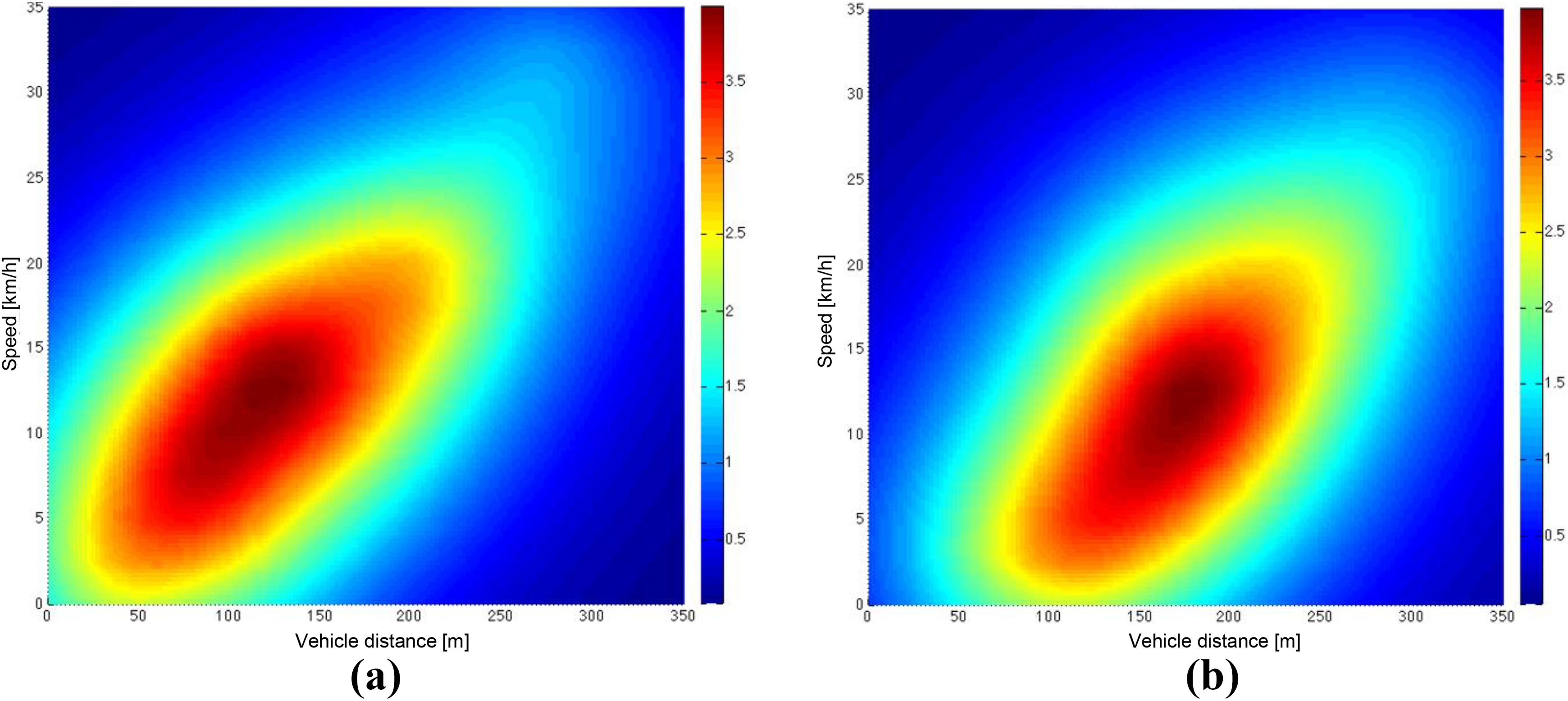
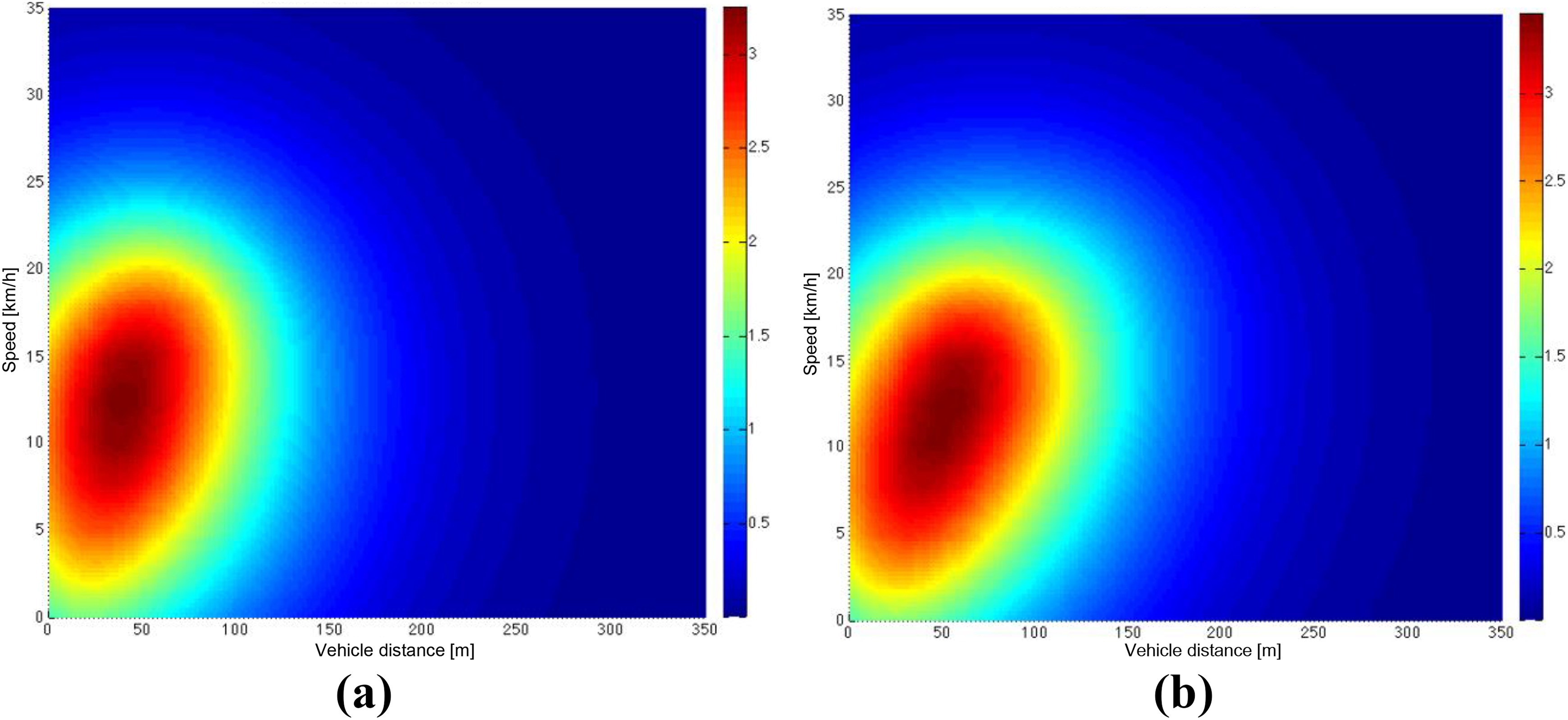
Driver A (female): diagram of the reward function under Japan 10–15 condition. (a) The result of randomly selected trial 1. (b) The result of randomly selected trial 2.

Figure 11.

Driver B (male): diagram of the reward function under NEDC condition. (a) The result of randomly selected trial 1. (b) The result of randomly selected trial 2. NEDC: New European Driving Cycle.

Figure 12.

Driver B (male): diagram of the reward function under Japan 10–15 condition. (a) The result of randomly selected trial 1. (b) The result of randomly selected trial 2.

Experiment analysis

The comparison of the results presented in Figures 9 to 12 obtained the following conclusions:

For the different tests of the same driver under the same condition, the shapes of reward functions are basically identical. This finding proves that the IRL algorithm has certain repeatability and can extract the characteristics of the car-following strategy of drivers.

For the same driver, the shapes of reward functions under different working conditions are the same, mainly due to the inconsistent state space under different conditions. For different conditions, the main part and the trend of the reward function of the same driver are basically the same. This finding indicates that the IRL algorithm does not depend on the specific conditions and can effectively extract the car-following characteristics.

The reward functions have completely different shapes for different drivers. The comparison of drivers A (Figures 9 and 10) and B (Figures 11 and 12) shows that as velocity increases, the distances corresponding to the peaks of two reward functions increase. For constant speed, the distance corresponding to the peak of the reward function of A is large, whereas the distance to the peak of the reward function of B is small. Therefore, the reward function of A is generally close to the coordinate axis of distance, and that of B is close to the axis of speed. This finding indicates that the car-following distance of the driving strategy of A is large, and that of B is small. In addition, the gradient of the reward function of A is small, and that of B is large. The reward function of driver A is shown in Figure 13, the reward function of driver B is shown in Figure 14, This finding indicates that A is less sensitive to changes in vehicle distance and speed, but B is more sensitive to the changing information.

Figure 13.

Reward function of driver A.

Figure 14.

Reward function of driver B.

Conclusions and future work

This work proposes the reward function R for drivers under different conditions by basing on the IRL algorithm and by combining the car-following data of two drivers. In addition, the visual verification and analysis of the reward functions are presented. First, preprocessing, analysis, and visualization of the car-following data are achieved. Second, the reward function is obtained in three steps: (1) The state space is determined, and the kernel function is transformed. (2) The reward function $R_{i, j}$ and the cumulative reward $V_{i, j}$ are calculated. (3) The weights of each reward function $R_{i, j}$ are determined, the IRL algorithm is designed, and the reward function R is obtained. Finally, the R of the two drivers under two conditions are visualized and analyzed, which proves the validity of the proposed algorithm. Through the analysis presented above, the characteristic of different people following a driving strategy is completely different. Thus, the specific car-following algorithm for each person should be designed according to their own characteristics. Based on the experimental verification in this article, IRL can obtain the reward function by evaluating the car-following data of drivers, analyzing their car-following characteristic, and achieving the specific car-following effect.

In future works, using the obtained reward function R, RL method is carried out to verify the car-following experiment.

Footnotes

Declaration of conflicting interests

The author(s) declared no potential conflicts of interest with respect to the research, authorship, and/or publication of this article.

Funding

The author(s) disclosed receipt of the following financial support for the research, authorship, and/or publication of this article: This work was supported by Junior Fellowships for Advanced Innovation Think-tank Program of China Association for Science and Technology under grant no. DXB-ZKQN-2017-035, Project funded by China Postdoctoral Science Foundation under grant no. 2017M620765, Project funded by China Postdoctoral Science Foundation Special Foundation under grant no. 2018T110095, the National Key Research and Development Program of China under grant no. 2017YFB0102603.

ORCID iD

Hongbo Gao

References

Yuan

. A study on driver’s vehicle-following model based on high speed real driving data. Auto Eng 2015; 6: 679–685.

Zhang

Wang

. Composite driver car-following model based on neural network approach. J Tsinghua Univ (Science Technology) 2008; 48(11): 1985–1988.

Liu

Sun

Guo

. Structured output-associated dictionary learning for haptic understanding. IEEE Trans Syst Man Cybern Syst 2017; 47(7): 1564–1574.

Reuschel

. Vehicle movements in a platoon. Oesterreichisch Ingen Arch 1950; 4: 193–215.

Wang

. Research of car-following behaviour and car-following model based on driving simulator. Master Thesis, Beijing Jiaotong University, China, 2013.

Gao

Zhang

Liu

. Cloud model approach for lateral control of intelligent vehicle systems. Sci Prog 2016; 24(12): 1–12.

Cole

. Linear quadratic game and non-cooperative predictive methods for potential application to modelling driver–AFS interactive steering control. Vehicle Syst Dynam 2013; 51(2): 165–198.

Pipes

. An operational analysis of traffic dynamics. J Appl Phys 1953; 24(3): 274–281.

Wang

. A framework of vehicle trajectory replanning in lane exchanging with considerations of driver characteristics. IEEE Trans Vehicul Technol 2017; 66(5): 3583–3596.

10.

Chandler

Herman

Montroll

. Traffic dynamics: studies in car following. Operat Res 1958; 6(2): 165–184.

11.

Herman

Montroll

Potts

. Traffic dynamics: analysis of stability in car following. Operat Res 1959; 7(1): 86–106.

12.

Zhang

Gao

. Multi-view clustering based on graph-regularized nonnegative matrix factorization for object recognition. Inf Sci 2017; 000(2017): 1–16.

13.

Gazis

Herman

Potts

. Car-following theory of steady-state traffic flow. Operat Res 1959; 7(4): 499–505.

14.

Gazis

Herman

Rothery

. Nonlinear follow-the-leader models of traffic flow. Operat Res 1961; 9(4): 545–567.

15.

May

Keller

HEM

. A deterministic queuing model. Trans Res 1967; 1(2): 117–128.

16.

Liu

Sun

Bin Fang

. Robotic room-level localization using multiple sets of sonar measurements. IEEE Trans Instrum Meas 2017; 66(1): 2–13.

17.

Ozaki

. Reaction and anticipation in the car following behaviour. In: Proceedings of the 13th international symposium on traffic and transportation theory (ISTTT), Lyon, 24–26 July 1993, pp. 349–366. Scientific Research.

18.

Olson

Rothery

. Deceleration levels and clearance times associated with the amber phase of traffic signals. Traffic Eng Inst Traffic Engr 1972; 42(7): 16–19.

19.

Gao

Zhang

Liu

. Longitudinal control for Mengshi autonomous vehicle via Gauss cloud model. Sustainability 2017; 9(12): 2259.

20.

Leutzbach

Wiedemann

. Development and applications of traffic simulation models at the Karlsruhe Institut für Verkehrswesen. Traffic Eng Control 1986; 27(5): 270–278.

21.

Kim

Lovell

Park

. Limitation of previous models on car-following behaviours and research needs. In: The 82th Transportation Research Board Annual Meeting, Washington D.C., USA, 12–16 January 2003.

22.

Gao

Zhang

. Research of intelligent vehicle variable granularity evaluation based on cloud model. Acta Elect Sinica 2016; 44(2): 365–374.

23.

Sutton

Barto

. Reinforcement learning: an introduction. Neural Netwk 2000; 13(1): 133–135.

24.

. Kernel-based least squares policy iteration for reinforcement learning. IEEE Trans Neural Netwk 2017; 18(4): 973–992.

25.

. Efficient reinforcement learning using recursive least-squares methods. J Artif Int Res 2002; 16: 259–292.

26.

Xie

Gao

Wang

. Vehicle trajectory prediction by integrating physics-and maneuver-based approaches using interactive multiple models. IEEE Trans. on Industrial Electronics 2017; 56(7): 5999–6008.

27.

Pyeatt

Howe

. Learning to race: experiments with a simulated race car. In: 11th International Florida Artificial Intelligence Research Society Conference, Sanibel Island, Florida, USA, 18–20, May, 1998.

28.

Liu

Sun

. Visual-tactile fusion for object recognition. IEEE Trans Auto Sci Eng 2017; 14(2): 996–1008.

29.

Loiacono

Prete

Lanzi

. Learning to overtake in TORCS using simple reinforcement learning. In: IEEE congress on evolutionary computation, Barcelona, Spain, 18–23 July 2010. IEEE.

30.

Riedmiller

. Neural fitted Q iteration–first experiences with a data efficient neural reinforcement learning method. Berlin: Heidelberg, 2005.

31.

Zheng

Liu

Guo

. A decision-making method for autonomous vehicles based on simulation and reinforcement learning. In: International Conference on Machine Learning and Cybernetics, Lanzhou, China, 13–16 July 2014.

32.

Gao

. A hardware platform framework for an intelligent vehicle based on a driving brain. Engineering 2018;4(2018):464–470.

33.

Abbeel

. Apprenticeship learning via inverse reinforcement learning. In: International conference on machine learning, 04–08 July 2004, pp. 1–8. ACM.

34.

Cole

. Game-theoretic modeling of the steering interaction between a human driver and a vehicle collision avoidance controller. IEEE Trans Human Mach Syst 2015; 45(1): 25–38.

35.

Gao

Cheng

Wang

. Object classification using CNN-based fusion of vision and LIDAR in autonomous vehicle environment. IEEE Trans Industr Inf 2018; 14(9): 4224–4231.

36.

Xing

. Hybrid-learning-based classification and quantitative inference of driver braking intensity of an electrified vehicle. IEEE Trans Vehicul Technol 2018; 67(7): 5718–5729.

37.

Dou

Fang

. A gated branch neural network for mandatory lane changing suggestion at the on-ramps of highway. IET Intelligent Transport Systems 2018 (in press).

Car-following method based on inverse reinforcement learning for autonomous vehicle decision-making

Abstract

Keywords

Introduction

Reinforcement learning and inverse reinforcement learning

Reinforcement learning

Inverse reinforcement learning

Design of IRL algorithm

Determine the state space and transform kernel function

Calculate reward function and cumulative reward

Determine the weights of reward function

Experiment and analysis

Experiment setup

Hardware and software

Environment modeling

Vehicle model

Experiment result

Experiment analysis

Conclusions and future work

Footnotes

Declaration of conflicting interests

Funding

ORCID iD

References