An adaptive approach to compensate seam tracking error in robotic welding process by a moving fixture

Abstract

Welding is one of the most common method of connecting parts. Welding methods and processes are very diverse. Welding can be of fusion or solid state types. Arc welding, which is classified as fusion method, is the most widespread method of welding, and it involves many processes. In gas metal arc welding or metal inert gas–metal active gas, the protection of the molten weld pool is carried out by a shielding gas and the filler metal is in the form of wire which is automatically fed to the molten weld pool. As a semi-metallic arc process, the gas metal arc welding is a very good process for robotic welding. In this article, to conduct the metal active gas welding torch, an auxiliary ball screw servomechanism is proposed to move under a welder robot to track the welded seam. This servomechanism acts as a moving fixture and operates separately from the robot. At last, a decentralized control method based on adaptive sliding mode is designed and implemented on the fixture to provide the desired motion. Experimental results demonstrate an appropriate accuracy of seam tracking and error compensation by the proposed method.

Introduction

Robotic welding can be of fusion or solid state types. Fusion methods in robotic welding mainly include tungsten inert gas, metal inert gas, laser, and submerged arc welding. Among these methods, metal active gas is a very appropriate process due to automatic filling of the electrode, high deposit rate, convenient welding quality, and inexpensive shielding gas for robotic welding and, therefore, is widely used in robotic welding industry. Researches in the field of robotic welding, especially in arc welding methods, are very wide and diverse. In general, robotic welding issues can be divided into two categories:

controlling the welding process and

controlling the motion of the welding torch, that is, tracking of the welding seam.

In process control studies, the control of the weld quality generated by controlling the welding variables and using process outputs such as sound, light, or welding current is considered. The control of weld geometry is one of the important areas of process control. ¹ The height of the weld bead is one of the most important geometric parameters of welding, and research has been carried out to control it. ² The model of arc welding processes is extremely complicated and nonlinear, hence the use of the neural network is of concern to researchers. ³ The control of the thermal energy entering the welding point and the width of the heat-affected area, which is very effective in the physical properties of the components, are the other issues in this area. ⁴

In torch motion control research (which is the concern of this research), the main problem is the detection and tracking of welding seams and control of the speed of the welding torch on the seam. In these studies, the seam detection method was studied using different sensors and methods such as machine vision and image processing, charge-coupled device camera, seam scanning using laser beam, mechanical seam detection methods, or welding current and voltage changes. ⁵

In seam detection using image processing, after seam detection, seam tracking error is corrected by robot. In this method, the accuracy is less than 1 mm in welding seam tracking. ^6,7 Laser vision sensor have been successfully employed in robust seam tracking. The feature point was obtained using the traditional morphological method before welding and determine the tracked region. ⁸ The method of morphological image processing was also accompanied by an object tracking algorithm and the measurement principle involved in the designed system was studied. ^9,10

To address the problem of low welding precision caused by the poor real-time tracking performance of common welding robots, a novel seam tracking system with excellent real-time tracking performance and high accuracy is designed based on a set of six-degree-of-freedom robotic welding automatic tracking platform to realize the real-time tracking of weld seams. Moreover, the feature point tracking method and the adaptive fuzzy control algorithm in the welding process were studied and analyzed. A laser vision sensor and its measuring principle were designed and studied, respectively.

In this study, a ball screw is used to compensate the tracking errors. Within modeling of the moving table, the accuracy required as well as the maximum frequency of the input path should be considered. Friction in ball screw systems suffers from a nonlinear, complex, and somewhat unknown nature. Hence, friction model can provide the required tracking precision by a control algorithm through a simple or complex model. So far, various models have been proposed for friction. ¹¹ Preventing any vibration in the moving system is essential to avoid the early failure of the ball screw. ¹² Also, for stable system performance, the closed loop bandwidth of the system should be appropriate to its natural frequency. ¹³ In general, due to the performance of the system, the controller type can be varied. Adaptive sliding mode controllers are among the most suitable ones for a ball screw mechanism. ^14,15 Another important issue is the flexibility of the mechanism. Flexibility reduces the achieved bandwidth of the system and many efforts have been made to solve this problem. ^16,17

In this article, a 480p webcam and image processing recognize the welding path. The seam tracking error is then compensated using an intermediate mechanism which moves the welding fixture with the workpiece. During the welding operation, the robot passes the welding torch nearby the seam, while the tracking error is compensated by the ball screw mechanism at the width of the welding seam.

Figure 1(a) illustrates the experimental components of the proposed robotic cell. As seen in this figure, a webcam camera, located in the upper part of moving table, captures the seam welding position relating the table and a robot marker. Data connection is shown in Figure 1(b), and a USB port and an appropriate protocol is used to transfer the 2-D images to the computer each 0.1 s. The position and speed of the table is also read through a serial port from a rotary encoder. A direct current (DC) motor serves to move the table and an adaptive algorithm is proposed to control the motion. As the welding operation starts, the necessary commands are simultaneously applied to the welding robot and the motor driver.The welding torch switches on when it arrives at the beginning of the trajectory, and the robot is programed to pass along a predetermined trajectory. The moving table changes the workpiece under the welding torch for that any complex seam and welding zone dimensions are precisely processed. Welding parameters are also set according to AWS Welding Hand Book.

Figure 1.

(a) Cell of robotic MAG (Metal Active Gas) welding and (b) separated robotic cell parts.

After giving a nonlinear ball screw mechanism governing dynamics in the third section of the article, a proportional–derivative (PD) controller based on adaptation law is proposed. The global asymptotic stability of this controller is analyzed and the table parameters are then identified using an estimator. Fifth section demonstrates the experimental results of the estimator and the controller and indicates its promising effect on the process quality.

Dynamic model of the mechanism

To control the moving table, firstly, it is necessary to select an appropriate model. Modeling of this mechanism can be either simple or complex with regard to the reference frequency, required accuracy, and available control bandwidth. Due to the accuracy required in this study, the thermal errors (increasing or decreasing the screw temperature that affects the lead), the hysteresis, and the flexibility of the nut, coupling, and screw are neglected. For modeling the mechanism, a linear non-frictional rigid model is chosen as described in equation (1). A suitable friction model has been added afterward.

${{\displaystyle T}}_{\text{motor}}=U=\left(\frac{{{\displaystyle J}}_{\text{motor}}+{{\displaystyle J}}_{\text{screw}}}{r}+r{{\displaystyle M}}_{\text{load}}\right)\ddot{x}$

1

As shown in Figure 2, T_motor and J_motor are the motor torque and moment of inertia, r and J_screw are the ball screw transmission ratio and moment of inertia, M_load is the load mass, and $\ddot{x}$ is the table acceleration. By adding the friction term to the above equation, the modeling can be completed. At sufficiently large speeds, the friction can be considered as a Coulomb-viscose type. At near zero speeds, the behavior of frictional forces is almost unknown. According to the form shown in Figures 3 and 4, Stribeak friction model, can suitably approximate the frictional forces around zero speeds. ¹⁸ The total friction force represented by F(v) is given by equation (2) as a function of the motion speed.

$F(v)=b\dot{x}+\left(F_C+\left(F_S-F_C\right)e^{{{\displaystyle -|\dot{x}/{{\displaystyle v}}_s|}}^{{{\displaystyle \delta }}_s}}\right).\text{sgn}\hspace{0.17em}(\dot{x})$

2

where F_c is the constant component of friction after the motion start (the Coulomb term), F_s is the dry friction component, and δ_s and v_s are the components related to the Stribeak friction. This equation describes the model; nevertheless, it is not completely appropriate to follow up the frictional force. Herein the presence of noise and delay in the speed sensor, the delay in the control loop, as well as the sampling rate at near zero speeds, can be quite troublesome. Therefore, another model is selected for the friction which is shown in equation (3). In Figure 5, the results of these two equations are compared against each other.

$F(v)=b\dot{x}\hspace{0.17em}+C\left(\frac{2}{\pi }\right)\mathrm{Arctan}\left({\left(\frac{\dot{x}}{\alpha }\right)}^9\right)$

3

Figure 2.

Scheme of a ball screw mechanism for the welding process.

Figure 3.

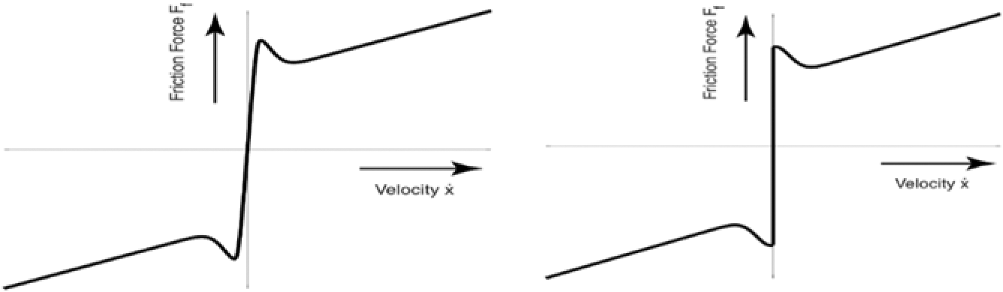
Stribeak friction model.

Figure 4.

Used friction model against Stribeak friction model results.

Figure 5.

Error in the friction model considering the model uncertainties.

As can be seen, this model creates a dead area near zero. α determines the width of the dead zone. This coefficient should be large enough to suit the noise, lag, sampling rate, and velocity. Considering this equation, the uncertainty component should be added to the model, which is larger than the modeling error. As a result, the selected friction model is expressed in equations (4) and (5) as follows

$U=a\ddot{x}+b\dot{x}\hspace{0.17em}+C\left(\frac{2}{\pi }\right)\mathrm{Arctan}\left({\left(\frac{\dot{x}}{\alpha }\right)}^9\right)+f$

4

$f\le F_s\left(1-|\left(\frac{2}{\pi }\right)\mathrm{Arctan}\left({\left(\frac{\dot{x}}{\alpha }\right)}^9\right)|\right)$

5

where a is the inertia coefficient of whole mechanism based on equation (1), b is the viscous friction coefficient, C is the Coulomb friction coefficient, U is the mechanism input torque, and f represents the unmodeled terms or model uncertainties.

Controller design

To design a controller for the mechanism, attention should be paid to the performance of the parametric and nonparametric uncertainties. Parametric uncertainties can be compensated using an adaptive controller. In this article, with the assumption that plant parameters are specified, a sliding mode controller has been used to deal with nonparametric uncertainties. For this purpose, a sliding surface is first defined in equations (6) and (7).

$S=\dot{\stackrel{\sim }{x}}+\lambda \tilde{x}$

6

$\ddot{x}=x-x_d={\left[\begin{array}{cc}\tilde{x}& \dot{\stackrel{\sim }{x}}\end{array}\right]}^{\text{T}}=-{\left[\begin{array}{cc}e& \dot{e}\end{array}\right]}^{\text{T}}$

7

By choosing the Lyapunov function as follows and putting its derivative in the following inequality, it gives

$\text{V}=0.5\hspace{0.17em}{S}^2$

8

$\dot{\text{V}}\le -\eta |S|$

9

The above inequality is extended and actually ensures getting the desired level during less than $\frac{S(0)}{2\eta }$ . ¹⁹ The control law will be achieved as in equation (10).

$U=b\dot{x}\hspace{0.17em}+C\left(\frac{2}{\pi }\right)\mathrm{Arctan}\left({\left(\frac{\dot{x}}{\alpha }\right)}^9\right)+a\left({\ddot{x}}_d+\lambda \dot{e}\right)-\left(a\eta +K\right).\text{sgn}\hspace{0.17em}(S)$

10

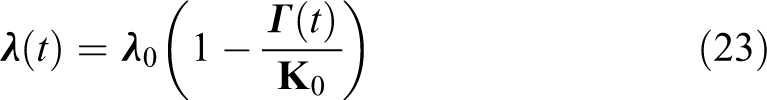
In these equations, λ is a constant and positive coefficient. Since this parameter takes the large values, the control effort is enlarged and tracking error quickly tends to zero. In the other hand, this value is limited due to the available control bandwidth and the motor saturation limit. K is another constant and positive coefficient and should be larger than the uncertainties term f. To avoid the chatter phenomenon, a convenient sliding surface should be adopted. In the equations, Φ is the boundary layer width, and the smallness of this parameter leads to oscillations and its largeness causes the tracking error incensement.

The above-mentioned control law, despite the convergence guarantee, is not very appropriate. Because the selection of small values for η, causes increased time to reach the surface for a large initial errors, and choosing large values for η, causes oscillations in small tracking errors (due to incomplete switching). The equation (11) could be rewritten as follows

$\dot{\text{V}}\le -\eta |S|-\beta S^2$

11

By considering β equals to aλ and iterating the previous steps and using the saturation function instead of the sign function, the control law changes as follows

$U=b\dot{x}\hspace{0.17em}+C\left(\frac{2}{\pi }\right)\text{arctan}\left({\left(\frac{\dot{x}}{\alpha }\right)}^9\right)+a\left({\ddot{x}}_d+\lambda \dot{e}+{\lambda }^{2}e\right)+\left(a\eta +K\right)\mathrm{s}at\left(\frac{\dot{e}+\lambda e}{\Phi }\right)$

12

By doing so, a PD controller has been added to the control law. By choosing some small values for η, at sufficiently large speeds, and by inserting the above controller to the mechanism, the tracking error varies as follows. Based on equation (13), the error differential equation indicates a complete tracking, and it exponentially converges toward zero

$\ddot{e}+2\lambda \dot{e}+{\lambda }^{2}e=0$

13

Parameters identification

Adaptive controllers are generally categorized into two categories of model reference and self-tuning controllers. Model reference controllers are not flexible enough despite the guarantee of parameters convergence. Indeed, in self-tuning controllers, the control law acts independently of the matching rule. Hence, in this article, self-regulating controller (due to its high flexibility) and the Least Square Estimation with exponential forgetting and bounded gain are used to estimate the vector of functions of parameters. In the self-regulating controllers, the output of the controller (force, torque, or controller output power) must first be defined according to the plant dynamic model. This output, which is the torque input into the mechanism, is linearly parameterized in terms of the vector functions of system parameters, as follows

$Y=WP$

14

where Y is the output torque of the motor, W is the row vector of the regression, and P is the column vector of the parameters. The first element of this vector is a, the equivalent inertia of the mechanism; the second element is the viscous friction coefficient; and the third one is the Coulomb friction coefficient. If the vector of estimated parameters are used in the above equation, equation (15) is achieved.

$\widehat{Y}=W\widehat{P}$

15

The result of the estimated tracking error is given as follows

$e_P=\widehat{Y}-Y$

16

If the output of the controller is considered as the applied torque into the mechanism, equation (17) is derived

$u=\left[ \ddot{x} \dot{x} \left(\frac{2}{\pi }\right)\text{arctan}\left({10}^6\dot{x} \right)\right]\left[\begin{array}{c}a\\ b\\ c\end{array}\right]=hP$

17

Since the acceleration of motion is not measurable, in the above equation, a first-order filter has to be applied as follows

$\left(\frac{1}{s+{\lambda }_f}\right)u=\left(\frac{1}{s+{\lambda }_f}\right)\mathbf{h}\mathbf{P}$

18

or

$u_f=h_{f}P, Y=u_f, W=h_f$

19

Also for the regressor vector, equation (20) is held

$h_f=W=\frac{\left[ \ddot{x} \dot{x} \left(\frac{2}{\pi }\right)\text{arctan}\left({10}^6\dot{x} \right)\right]}{S+{\lambda }_f}=\frac{\left[ S\dot{x} \dot{x} \left(\frac{2}{\pi }\right)\text{arctan}\left({10}^6\dot{x} \right)\right]}{S+{\lambda }_f}=\left[ \dot{x}-{\dot{x}}_f {\dot{x}}_f {\left(\left(\frac{2}{\pi }\right)\text{arctan}\left({10}^6\dot{x} \right)\right)}_f\right]$

20

Now, using the following vector, one can update the vector of parameter functions ¹⁹

$\dot{\widehat{\mathbf{P}}}=-\Gamma \left(t\right)W^T{e}_p$

21

$\dot{\Gamma }\left(t\right)=\lambda \left(t\right)\Gamma \left(t\right)-\Gamma \left(t\right)W^{T}W\Gamma \left(t\right)$

22

$\lambda \left(t\right)={\lambda }_0\left(1-\frac{\Gamma \left(t\right)}{K_0}\right)$

23

where Γ is the square diagonal matrix of the gain of the parameter updates, and the square diagonal matrix λ is the forgetting gain matrix. By increasing the initial value of this matrix, the convergence of the parameters will be faster. To evaluate the estimator’s performance, a simulation has been conducted.

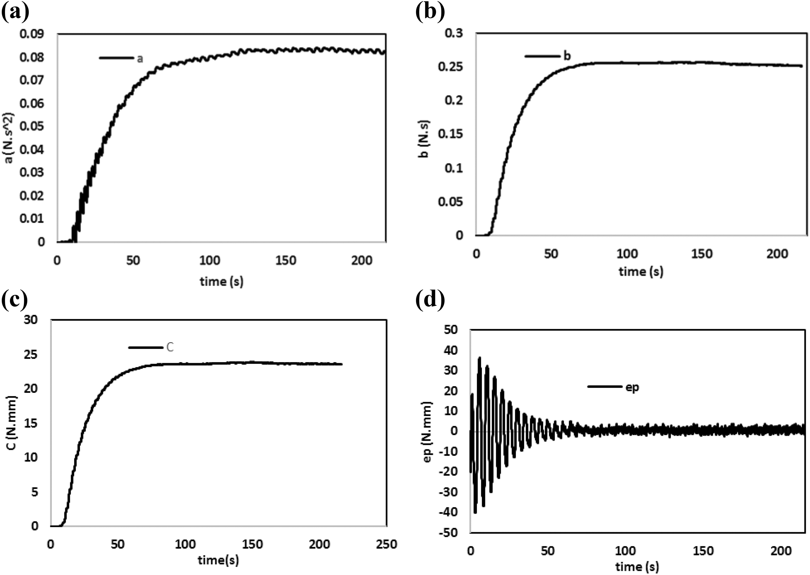
The simulation results of the MATLAB^® [version R2015a]/Simulink environment are presented in Figure 6. The diagrams in this figure show the convergence of the plant parameters. As can be seen, due to the absence of noise and sensor lags, the magnitude estimates are selected sufficiently large. Consequently, the convergence of the parameters has been completely tended to zero in a very short time, and the tracking error equals absolutely to zero. But, due to the noise and delay, as well as the low sampling rate, one have to choose small gain coefficients for the estimator. Consequently the convergence of parameters occurs over a longer period.

Figure 6.

Simulation of the estimator performance for (a) a, (b) b, (c) ep and (d) c.

Experimental results

To implement the controller, the LabVIEW^® [version 2014] software is used. The path extracted from the camera is not an appropriate input for the controller, since this trajectory is discrete and the curve derivatives are not available. Therefore, an appropriate curve of data must first be extracted. The B-spline type curve is suitable considering the analytical characteristics. ²⁰ Because this curve has a simple formulation and because it does not pass through the data, it is able to eliminate data noise and is very useful in this study. Speed data and table position are read through the serial port of the motor driver, and the control command is sent as an analog signal via the data acquisition (DAQ) card to the driver. The following figure shows this process.

The welding path is not sufficiently rich to estimate the parameters; therefore, before the start of the welding operation, a sinusoidal pathway like $r=100\text{sin}\left(t\right)$ is used to update the parameters. Also due to the discrete time of the controller and also because the duration of each controller loop is 40 ms, the first-order and integrator filter is used as follows ²¹

$\text{G}\left(z\right)=\frac{0.04}{1-0.97z}$

24

$\text{G}\left(z\right)=\frac{0.04}{1-z}$

25

Figure 7 gives a general vision on the control scheme in the applied software. Also, the diagrams of Figure 8 show the estimation results. Because of the delay in sensors and the actuator, as well as the high torque oscillations in the electrical motor, small gains are used for the estimator, and as a result, the convergence of parameters over time is much higher than the simulation.

Figure 7.

Process consequence in control execution inside LabVIEW environment.

Figure 8.

Experimental results of the estimator for (a) a, (b) b, (c) ep and (d) c.

As can be seen, all parameters converge to the desired values. The prediction error is due to torque oscillations, sensor and sensor delays, and variations around zero. To evaluate the performance of the controller, a sinusoidal path like $r=100\text{sin}\left(0.6t\right)$ is used, which is similar to the welding path in Figure 9. Sensor and actuator delays, as well as high torque oscillations, cause a large number of detected errors. Using the right experimental equipment, much less error can be achieved.

Figure 9.

Experimental results of tracking the sinusoidal trajectory.

At last, Figure 10 shows the sample of a welded piece using the mechanism and controller used.

Figure 10.

A sample of workpiece before (a) and after (b) welding.

The uniformity of the geometry of the welds achieved in this method (width and height of the bead) is technically acceptable. The welds are tested in terms of other visible defects, such as surface cracks and melt spraying. In the diagram of Figure 11, the width of the bead is given for different points of the weld path. It is observed that the weld uniformity is very desirable, and the presence of defects is also convenient.

Figure 11.

Width variation along the weld bead.

Conclusions

Arc welding processes are one of the most common and complex manufacturing processes. The quality of the welds is affected by many variables and much expertise is needed to create high quality welds. Also, welding created by skilled welders does not have much repeatability. Therefore, the use of a robot for welding has been of great interest to many.

The conductivity of welding torch on the seam is one of the challenges in this field. In this article, to compensate for the seam welding tracking error, a decentralized ball screw system that cooperates with a robot was proposed. A 480p camera was used to recognize the seams. To control the mechanism, an adaptive sliding controller was applied, and the mechanism parameters were also identified via an adaptive algorithm. In summary, the seam tracking error was less than 1 mm, which can be reduced using appropriate equipment in future studies.