Sage Journals: Discover world-class research

Abstract

Self-localization in autonomous robots is one of the fundamental issues in the development of intelligent robots, and processing of raw sensory information into useful features is an integral part of this problem. In a typical scenario, there are several choices for the feature extraction algorithm, and each has its weaknesses and strengths depending on the characteristics of the environment. In this work, we introduce a localization algorithm that is capable of capturing the quality of a feature type based on the local environment and makes soft selection of feature types throughout different regions. A batch expectation–maximization algorithm is developed for both discrete and Monte Carlo localization models, exploiting the probabilistic pose estimations of the robot without requiring ground truth poses and also considering different observation types as blackbox algorithms. We tested our method in simulations, data collected from an indoor environment with a custom robot platform and a public data set. The results are compared with the individual feature types as well as naive fusion strategy.

Keywords

Localization feature selection expectation maximization bag of words

Introduction

Robot navigation has an important place in the development of intelligent and autonomous robots. The robots need to recognize and model their surroundings and estimate their position within this model to accomplish complex tasks and make decisions. The localization problem is the estimation of robot pose within the known map of the environment based on sensory observations. The probabilistic approaches for solving this problem involve definition of an observation model, which compares observed data with the map and defines a similarity between them. In most of the applications, instead of using the raw sensory data directly in the observation model, a feature extraction process collects useful and more compact information to be used as observations. In this article, feature is used as a general term and refers to the compact information extracted from some raw sensory data. As an example, a color histogram may be extracted from an image or straight lines and corners may be extracted from the raw laser scans. When developing a localization algorithm, the designers usually decide on a feature extraction method, which aligns with the assumptions about the current environment. However, the same method may not perform well in a different environment, and another feature extraction method might have to be selected by the designers. Automating this feature type selection process for different environments would make the localization system easier to deploy into new places and increase robustness in heterogeneous environments.

In the context of localization, the desired attributes of a feature extraction method are to produce information which has a low systematic error against the dynamism in the environment (e.g. color histograms may be consistently wrong based on the known map with changing light conditions, hence has high systematic error) and to carry out this robustness into various types of places the robot operates. While there may be several types of sensors and feature extraction methods with strengths and weaknesses for a particular environment, as the diversity of the environment increases, it becomes challenging for a particular feature extraction method to perform well in all places. With this intuition, in this work, we propose a method for autonomous selection of feature types based on the environment without any supervised information in the localization setting. The framework treats feature types as independent blackbox methods, and instead of modifying or tuning the feature extraction method for a particular environment, it aims at improving the localization accuracy by fusing features from different sources in the observation model. We also assume that the map (and its quality) is tied to the feature extraction method and given to the framework (i.e. it is not estimated along with the robot pose).

The widely accepted solutions to the self-localization problem originates from probabilistic modeling and Bayesian filtering. The metric approaches estimate the robot pose in a continuous state space (CSS) and model the environment with spatial objects or quantized obstacle locations. The Extended Kalman Filter (EKF)^1,2 assumes a Gaussian distribution on all variables, and Monte Carlo Localization (MCL)^3,4 relaxes this assumption with a nonparametric distribution by utilizing Particle Filters. On the other hand, topological approaches represent the possible poses of the robot as a set of discrete places and the environment as the compact descriptions of these places.^5

–8 With the range sensors, the observation models include scan matching,^9,10 possibly with likelihood field representation¹¹ or line¹² and corner extraction.¹³ The visual sensors are utilized in landmark extraction methods with features such as scale-invariant feature transform (SIFT)^14,15 and speeded up robust features (SURF),^16,17 which provide robust descriptors against changes in viewpoints. In the topological approaches, observation models based on place similarity have become more popular. With the visual sensors, image retrieval algorithms with color histograms¹⁸ or Bag of Words (BoW) representations^19
–21 prove to be viable choices for comparing appearances. With these methods, topological navigation systems evolved toward utilizing more sparse and qualitative representations, and this allowed larger scale operations and longer term autonomy. These effects are more pronounced in more recent works.^22,23 As will be discussed later, our optimization algorithm assumes a finite and discrete set of poses as its input; therefore, we formulated our method on topological localization with discrete Bayes Filter and MCL with a set of particles. In the real-world implementation, we used image similarity with SIFT descriptors and BoW representation, and likelihood field based scan similarity for the range sensor, and compared the localization accuracy with the performance of individual feature types. We tested the MCL algorithm in a simulated landmark-based map environment.

Using more than one sensor type in robot navigation is extensively studied in sensor fusion literature for a variety of benefits such as improving accuracy, recovering from failures, and extended coverage.²⁴ From the perspective of localization and mapping, the works on sensor fusion can be grouped into feature level fusion and filter level filters.²⁴ In the feature level approaches, extracted features from different sensors are processed together to generate more informative features, and they usually exploit the domain and sensor specific properties. In Castellanos et al.’s study,²⁵ associations between different sets of landmarks are established by considering their Gaussian uncertainties. In Deelertpaiboon and Parnichkun’s work,²⁶ uncertainties are represented and fused with fuzzy membership functions. In the filter level approaches, different features directly contribute to the estimation of the target variables, hence uncertainties are augmented in the probabilistic model of the filter.²⁴ These approaches have the benefit of augmenting the filter with latent variables to increase accuracy of the assumptions in the model. In Zhu et al.’s work,²⁷ sensor biases are estimated with Variational Bayesian algorithm and in Caron et al.’s work,²⁸ the switching observation model is used to recover from changing sensor states. While our approach is also a filter level approach, it models the feature quality based on the environment and weighs them in a complementary way.

The expectation–maximization (EM) algorithm is an iterative batch algorithm for maximum likelihood estimations.^8,29 The method is particularly useful when there are unknown latent variables in the problem. The algorithm involves an expectation step (E-step) where the latent variables are estimated and then followed by a likelihood maximization step (M-step) based on the estimated latent variables. This factorization of variables is particularly convenient for the simultaneous localization and mapping (SLAM) problem, where the distribution of the robot trajectory is estimated in the E-step and the most likely map is estimated in the M-step.^8,30 Some other latent variable types are: the loop closure constraints in a topological mapping model in the study by Lee et al.³¹ and landmarks being dynamic or not in the study by Rogers et al.³² In our approach, the latent variables are the indicators of the best quality feature for current region.

The rest of the article is organized as follows. In second section, we introduce the problem statement, modified probabilistic model, formulation of the EM algorithm, and feature types used in the real world. In third section, we describe our experiment environment and report the results from the simulation environment, real-world, and public data set. In fourth section 4, we conclude the contributions of this work.

Proposed approach

Basic localization model

In this section, we start by stating the probabilistic model of the localization problem, which is an instance of the recursive state estimation problem.³³ Let the random variable $s_{t}$ represent the state of the robot at time t. In localization problem, the state is the location of the robot. We will focus on two different representations of the location later in this section, until then it will be called state. An observation $o_{t}$ , taken at time t depends on the current state of the robot $s_{t}$ with the probability distribution $p (o_{t} | s_{t})$ . Similarly, the robot pose $s_{t}$ depends on the previous robot pose $s_{t - 1}$ with the probability distribution $p (s_{t} | s_{t - 1})$ . The graphical representation of the model is given in Figure 1. In a more detailed model, the control input (e.g. odometry readings of the robot) can also be included in state transition as a control input in the state transition, but it has little relevance to the outcome of our approach, and therefore, it is omitted for simplicity.

Figure 1.

Graphical representation of the classical localization problem. At each discrete time step, the observation $o_{t}$ depends on the current robot state $s_{t}$ , which depends on the previous state $s_{t - 1}$ .

The state transition model $p (s_{t} | s_{t - 1})$ and the observation model $p (o_{t} | s_{t})$ are considered to be known and the problem is to estimate $p (s_{t} | o_{1 : t})$ , namely the probability of the robot state given all past observations. This distribution is also called belief of the robot, $b e l (s_{t})$ .

The state of the robot, based on the application, can be represented in different ways, and we developed our algorithm for two cases: a discrete state space (DSS) and a CSS representation. The discrete case manifests itself in topological approaches and the possible locations of the robot form a discrete finite set of places. These can be considered as nodes in a graph, where edges may represent the spatial relations between places. While each place can be attributed with some physical position, for our purposes, they are simply represented as a discrete index, that is, $s_{t} \in {1, 2, 3, \dots, N}$ for N places. The belief at time t is given as a list of probability values

b e l_{dss} (s_{t}) = (τ_{t,1}, τ_{t,2}, τ_{t,3},..., τ_{t, N})

where $τ_{t, l}$ is the probability that robot is in ${place}_{l}$ at time t. At each new time step, the probabilistic localization algorithm computes the new belief distribution using the previous belief distribution and variable dependencies given in Figure 1 in two steps. The first step is called prediction and it computes $p (s_{t} | o_{1 : t - 1})$ , that is, the new belief state before integrating the most recent observation. It follows from the definition of conditional probability given the previous state, $s_{t - 1}$ as

p (s_{t} | o_{1 : t - 1}) = \sum_{i}^{N} p (s_{t} | s_{t - 1} = i) p (s_{t - 1} = i | o_{1 : t - 1})

where first term is the state transition model (assumed to be known) and the second term is the previous belief state, and the summation is defined over all possible values of the previous state. The second step of the localization formulation is called the correction step, where the predicted belief state is corrected with the observation model. Using Baye’s rule on the belief state (inverting variables $s_{t}$ and $o_{t}$ ) we get

p (s_{t} | o_{1 : t}) = \frac{p (s_{t} | o_{1 : t - 1}) p (o_{t} | s_{t}, o_{1 : t - 1})}{p (o_{t} | o_{1 : t - 1})}

where $p (s_{t} | o_{1 : t - 1})$ is the predicted belief state from the previous step. The term $p (o_{t} | s_{t}, o_{1 : t - 1})$ only depends on $s_{t}$ and the term $p (o_{t} | o_{1 : t - 1})$ does not depend on $s_{t}$ , so the equation (3) can be simplified into

p (s_{t} | o_{1 : t}) \propto p (s_{t} | o_{1 : t - 1}) p (o_{t} | s_{t})

In the continuous state space case, in a 2-D map, the state is the tuple $〈 x, y, θ 〉$ for position $x, y$ and bearing $θ$ also called robot pose. In MCL algorithm,³⁴ the belief is represented as a set of particles

b e l_{css} (s_{t}) = {ρ_{t,1}, ρ_{t,2}, ρ_{t,3}, \dots, ρ_{t, M}}

where $ρ = 〈 \dot{x}, \dot{y}, \dot{θ} 〉$ is a pose sample. At each new time step, the predicted belief state is approximated by sampling each particle from the state transition model

p (s_{t} | o_{1 : t - 1}) = {sample {\hat{ρ}}_{t, i} \sim p (s_{t} | s_{t - 1} = ρ_{t - 1, i}) : \forall i}

where for each particle, a new random particle is sampled from the distribution $p (s_{t} | s_{t - 1} = ρ_{t - 1, i})$ . In the correction step, for each particle, a weight is calculated using the particle and observation model (i.e. the likelihood of observing the current observation at given particle pose), and the particle set is resampled based on their weights as

w_{i} = p (o_{t} | s_{t} = {\hat{ρ}}_{t, i})

p (s_{t} | o_{1 : t}) = {draw ρ_{t, i} with probability w_{i} : \forall i}

Note that, for simplicity, the weights ( $w_{i}$ ) are not included inside the particle set in $b e l_{css} (s_{t})$ and only calculated for predicted particles ( $\hat{ρ}$ ) before the resampling step. This is equivalent to associating a uniform weight to all particles, provided the resampling step is performed at each iteration.

The DSS and CSS are illustrated in Figure 2. The navigation of the robot from start to finish is called an episode. We also assume, without loss of generality, that the environment has different characteristic at various regions. Each region is a subset of all possible states (places or poses), and the function

r (s) \in {1, 2, \dots, L}

Figure 2.

Illustration of DSS and CSS. Dashed line represents the actual path of the robot. The DSS is formed by N places, and the belief at time t is a list of probability values ( $τ_{t,1 : N}$ ). In CSS, the state is the pose of the robot, and belief state is the set of particles ( $ρ_{t,1 : M}$ ). A region is a subset of locations or places in the environment, and dotted lines represent their boundaries. DSS: discrete state space; CSS: continuous state space.

maps states to L possible regions (e.g. rooms). This function is considered available (e.g. “Region change detection” section) but not used for constraining the belief distribution, instead will be useful in “Multiple feature types” section.

Also note that we don’t provide a formal definition of map, instead assume the observation model $p (o_{t} | s_{t})$ provides the probability distribution using feature type specific external information. In real-world implementations of DSS case, each place is associated with some map features collected from a prior mapping episode, and later in the localization episode, an observation is compared with the associated features for all places. In the simulation implementation of CSS case, there is no separate mapping episode, the map is a set of landmarks, which can be observed at poses close to their locations.

Multiple feature types

In the basic localization model, the observation $o_{t}$ represents all possible sensory information available. This may be a multi-dimensional vector, and the product of processing the raw sensory data, namely the feature extraction process. Now let us consider that the observations are the products of K separate feature extraction processes. There can be different sensor hardware installed and their raw data can be processed in a different way or the data from the same sensor might be processed with different feature extraction algorithms, resulting with different observation types. The observation $o_{t}$ can be split into K different variables $o_{t}^{1}, o_{t}^{2}, \dots, o_{t}^{K}$ , each representing a different feature type and has its own observation model $p (o_{t}^{i} | s_{t})$ . Note that each observation $o_{t}^{i}$ can be a multi-dimensional vector (e.g. bins in a histogram). The individual feature extraction algorithms and by extension the associated observation models are considered as black box processes in the context of the problem model.

Let us also assume, without loss of generality, that in each region, one feature type is better suited to be used as opposed to others. To model this, we introduce a discrete variable $b_{t} \in {1, 2, \dots, K}$ , which indicates the best feature type at that time t. We also assume that

b_{t} = b_{u} if r (s_{t}) = r (s_{u})

which basically states that the variable b is uniform inside the same region. The modified graphical model is given in Figure 3 in the case of two feature types.

Figure 3.

Graphical representation of the modified model with $K = 2$ . And $b_{t}$ indicates the best feature type for time t and is hidden.

With the new model, the observation model is given as

p (o_{t} | s_{t}, b) = \sum_{i = 1}^{K} p (o_{t}^{i} | s_{t}, b_{t} = i) p (b_{t} = i)

The new observation model simply selects the best feature type, indicated by $b_{t}$ , in the current region. The focus of our approach is to estimate $p (b)$ , namely the best feature type for each region in the environment.

Optimization with EM

In practical localization applications, the observation model is often implemented as a likelihood function instead of a probability distribution, the difference being likelihood function does not have to integrate to 1. Inspection of equation (11) reveals that the combined likelihood at any time is the weighted average of the individual likelihoods of the feature types. We can write the observation model in likelihood function form as

g (o, s) = \sum_{i = 1}^{K} f_{i} (o^{i}, s) h_{i} (s)

where

f_{i} (o^{i}, s) \approx p (o_{t}^{i} | s_{t}, b_{t} = i)

represents the likelihood function for feature type i,

g (o, s) \approx p (o_{t} | s_{t}, b)

represents the combined likelihood and

h_{i} (s) = p (b = i | s)

represents the weight of feature type i for robot position s, which also satisfies

\sum_{i = 1}^{K} h_{i} (s) = 1

Furthermore, with the assumption that the weights are uniform across a region with equation (10), the weight function becomes a table

h_{i} (s) = α_{i, j} where j = r (s)

with $K \times L$ elements, where L is the number of regions.

In this form, the problem is to estimate $α_{i, j}$ for each feature type and region on the map. If the ground truth states of the robot were available, it would be possible to model the problem as a nonlinear optimization problem, where the trajectory error represents the objective function to be minimized, and weights represent the free variables to be optimized, and solve with an optimization algorithm such as Evolutionary Strategies.³⁵ Instead, we present and approximate the EM algorithm that exploits the nature of the localization model and does not require ground truth locations. Each iteration of the optimization algorithm requires recomputation of state probabilities for the entire episode. We first introduce the algorithm with the DSS notation and then describe the equivalent algorithm for the continuous state space case.

The weights are trained iteratively in two steps. For simplicity let α represent all the weights $α_{i, j}$ .

E-Step. In this step, the localization algorithm is performed and place probabilities are calculated for $t = 1 : T$ as

τ_{t, l} = p (s_{t} = l | o_{1 : t}, α)

M-Step. In this step, the weights are selected that maximize the joint probability of observations and states.

α^{new} = arg max_{α} (log p (o_{1 : T}, s_{1 : T} | α))

\approx arg max_{α} (log \sum_{t} \sum_{l} (p (o_{t} | s_{t} = l, α) p (s_{t} = l | o_{1 : T}, α)))

The term $p (o_{t} | s_{t} = l, α)$ is the observation model, which can be replaced with equation (14) and the second term $p (s_{t} = l | o_{1 : T}, α)$ can be replaced by the belief state from the expectation step (equation (18))

α^{new} \approx arg max_{α} (log \sum_{t} \sum_{l} g (o_{t}, l) τ_{t, l})

When we also substitute equations (12) and (17) into equation (21), we get

α^{new} \approx arg max_{α} (log \sum_{t} \sum_{l} τ_{t, l} \sum_{k} f_{k} (o^{k}, l) α_{k, r (l)})

To maximize equation (22), we follow an approximate approach based on counting the strong feature type for the entire episode and maximize the term $\sum_{k} f_{k} (o^{k}, l) α_{k, r (l)}$ . To explain it, we first define a helper function to sort likelihoods of a particular feature type. For each time step t, let $rank (o_{t}^{k}, l) \in [1, 2, \dots, N]$ represent the order of likelihood value $f_{k} (o_{t}^{k}, l)$ in the descending sorted list formed by all possible values of L (places) such that

rank (o_{t}^{k}, u) < rank (o_{t}^{k}, v) \Leftrightarrow f_{k} (o_{t}^{k}, u) > f_{k} (o_{t}^{k}, v)

The value of this function is 1 if the likelihood of a feature type at time t is the highest for that particular place, among other places (and it has the value of N if it has the lowest value). The rank function is useful in comparing different types of likelihood functions with possibly different scaling on the basis of current place. With the help of the rank function, let us also define an indicator function

I (o_{t}, k, l) = {\begin{array}{l} 1 & if rank (o_{t}^{k}, l) = {min}_{j} rank (o_{t}^{j}, l) \\ 0 & otherwise \end{array}

The function $I (o_{t}, i, l)$ at time t is 1 if the feature type K has the lowest rank value among other feature types for the place L and 0 otherwise. In other words, the indicator function selects the most confident feature type for a particular place. In the maximization step for region j, the updated weight $α_{i, j}^{new}$ for feature type i is given as

α_{i, j}^{new} = \frac{1}{η_{j}} \sum_{t} \sum_{l \in {region}_{j}} τ_{t, l} I (o_{t}, i, l)

where

η_{j} = \sum_{i} α_{i, j}^{new}

Equation (25) evaluates the number of times, in the course of an episode, a feature type is considered best for a particular place, weighted with the probabilities of that place. The numbers used in computation of $α_{i, j}^{new}$ are described in Figure 4.

Figure 4.

The values used in computation of $α_{i, j}^{new}$ for $K = 2$ , illustrated for two time steps out of $1 : T$ . For each place inside the indicated region, the indicator $f_{i} > f_{j}$ evaluates to 0 or 1 and multiplied by the τ values.

Figure 5.

A sample image and the corresponding keypoints. The distribution of keypoints (histogram) over clusters forms the observation for that place.

The weight optimization algorithm is given in Algorithm 1. Note that we kept the function notation instead of defining redundant variables for simplicity. The EM iteration is repeated until change in weights is sufficiently low. Note that training is a batch algorithm and can be incrementally performed again with the new episodes. In Algorithm 5, the complexity of lines from 4 to 10 is $O (N K)$ , where N is the number of places and K is the number of feature types. Lines 11 to 13 has the complexity $O (K N log (N))$ , assuming sorting would require $O (N log (N))$ complexity. Therefore, one iteration of the EM loop (lines 3 to 15) has the complexity $O (T (N K + K N log (N))) = O (T K N log (N))$ , where t is the number of time steps in the localization episode. Number of EM iterations required until convergence does not directly depend on variables N, K, or t, and in our experiments, it was typically between 5 and 10 iterations.

Algorithm 1.

Weight optimization (DSS case).

Input:

o_{1 : T}

Output: Optimized α

1: Initialize α close to uniform distribution for all regions

2: repeat

3: for

t = 1

to t do {Time}

4: for

l = 1

to N do {Places}

5: for

k = 1

to K do {Feature types}

6: Compute

f_{k} (o_{t}, l)

, keep value.

7: Accumulate

f_{k} (o_{t}, l) α_{k, r (l)}

into

g (o_{t}, l)

as the combined observation model (equation (12))

8: end for

9: Update

τ_{t, l}

using

g (o_{t}, l)

and

τ_{t - 1, 1 : N}

(equation (2))

10: end for

11: for

k = 1

to K do {Feature types}

12: Sort

f_{k} (o_{t},1 : N)

and assign ranks (equation (23))

13: end for

14: Increment

α^{n e w}

table for time t with indicators weighted by

τ_{t,1 : N}

(equation (25)).

15: end for

16:

α \leftarrow

normalized

α^{n e w}

17: until Change in α is small

Application to MCL

In MCL, the probability distribution over the continuous state space is represented with the set of finite particles instead of parameterization as a known distribution. This gives the ability to define an estimator over the state space using samples instead of complete analytical solution. Notice that in the equation (22), the operation is an accumulation over all possible places, weighted by their probabilities. With the particle set, the same operation can be defined using particles and their weights, over all possible poses. The term $τ_{t, l}$ in the equation (22) can be replaced with particle weights $w_{t,1 : M}$ and the summation is defined over the particles $ρ_{t,1 : M}$ as

α^{new} \approx arg max_{α} (log \sum_{t} \sum_{l} w_{t, l} \sum_{k} f_{k} (o^{k}, ρ_{t, l}) α_{k, r (ρ_{t, l})})

and equation (25) can be replaced as

α_{i, j}^{new} = \frac{1}{η_{j}} \sum_{t} \sum_{ρ_{t, l} \in {region}_{j}} w_{t, l} I (o_{t}, i, ρ_{t, l})

And finally the $rank (o_{t}^{k}, ρ_{t, l})$ function is used for sorting feature likelihoods throughout the particles. The new algorithm with MCL is given in Algorithm 2. The complexity of this algorithm is very similar to the discrete case; instead of N possible places, now there are M particles, so the complexity is given as $O (T K M log (M))$ .

Algorithm 2.

Weight optimization (CSS case).

Input:

o_{1 : T}

Output: Optimized α

1: Initialize α close to uniform distribution for all regions

2: repeat

3: for

t = 1

to t do {Time}

4: for

i = 1

to M do {Particles}

5: Sample

{\hat{ρ}}_{t, i}

using state transition (equation (6))

6: for

k = 1

to K do {Feature types}

7: Compute

f_{k} (o_{t}, {\hat{ρ}}_{t, i})

, keep value.

8: Accumulate

f_{k} (o_{t}, {\hat{ρ}}_{t, i}) α_{k, r ({\hat{ρ}}_{t, i})}

into

w_{t, i}

as the combined weight (equation (7))

9: end for

10: end for

11: for

k = 1

to K do {Feature types}

12: Sort

f_{k} (o_{t},1 : N)

and assign ranks (equation (23))

13: end for

14: Increment

α^{n e w}

table for time t with indicators weighted by

w_{t,1 : M}

(equation (25)).

15: Resample particles using weights

w_{t,1 : M}

16: end for

17:

α \leftarrow

normalized

α^{n e w}

18: until Change in α is small

Real-world features

In the application of the discrete localization model to the real world, two feature extraction algorithms are selected for a color camera and a 2-D laser scanner. The feature types are selected based on their compatibility with the discrete state representation. The process has two steps. In the first step, called mapping episode, the robot is navigated through the environment with reasonable coverage of the environment and during navigation, a new place is created at regular displacements of the robot and associated with features collected at that place. The features collected in this step represent the map and used in the second step. In the second step, the robot is navigated through a similar path, the features are collected again for discrete places and used as observations to localize the robot in the generated map from the first step. The second step will be referred as the localization episode.

To measure the localization error, each place in the localization episode must be associated with a place in the mapping episode. To achieve this, in our experiments, we manually navigated the robot as close to the mapping trajectory as possible but that alone does not ensure unambiguous association. Therefore, we manually identified real-world correspondences between the two episodes and interpolated the rest of the trajectory to obtain ground truth for the localization episode.

In the rest of this section, the likelihood functions $f_{camera} (image, s)$ and $f_{laser} (laser, s)$ are given.

Camera features

For the camera sensor, the BoW¹⁹ representation is widely used in localization and SLAM applications. BoW allows compact representation of scenes and robust comparison with other scenes. The application of BoW requires a training step before forming the map and observations.

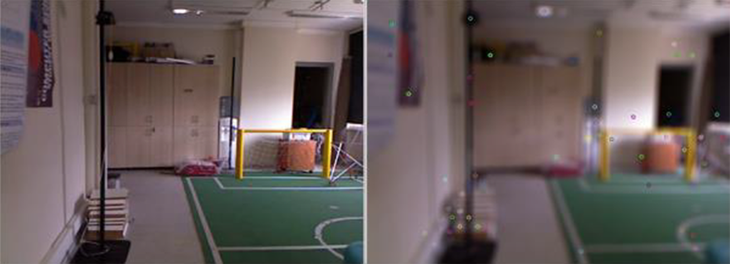
In the training step, for each place in the mapping episode, the corresponding image is processed and SIFT keypoints are collected along with their descriptors. Once all of the places are created and the mapping phase is finished, the keypoints collected from the entire episode are clustered with the K-Means algorithm into a certain number of groups. Once the clustering is finished, for each image, a histogram is calculated which represents the number of keypoints assigned to each cluster within that image. The calculated histogram is then associated with the place. A sample image and the corresponding keypoints are given in Figure 5. Note that the image is blurred to lower the noise caused by the robot motion.

Figure 6.

A sample laser scan, extracted lines (right) and corresponding likelihood field (left). Darker points have higher probability.

In the localization episode, for each image from a place, the histogram is calculated with the cluster centers built in the training step. The histogram is then compared with all the histograms from the mapping episode and the comparison results are used as the observation model (probability distribution over all possible places).

There are two widely used methods for histogram comparison. Let $z_{1}$ and $z_{2}$ represent two histograms and $z_{1} (i)$ represents the number of keypoints in the cluster center i. The first method for calculating the correlation is given as

d (z_{1}, z_{2}) = \frac{\sum_{i} (z_{1} (i) - {\bar{z}}_{1}) (z_{2} (i) - {\bar{z}}_{2})}{\sqrt{\sum_{i} {(z_{1} (i) - {\bar{z}}_{1})}^{2} \sum_{i} {(z_{2} (i) - {\bar{z}}_{2})}^{2}}}

{\bar{z}}_{k} = \frac{1}{C} \sum_{i} z_{k} (i)

where C is the number of cluster centers. Another method for comparing histograms is the χ ² method given as

d (z_{1}, z_{2}) = \sum_{i} \frac{{(z_{1} (i) - z_{2} (i))}^{2}}{z_{1} (i)}

While the χ ² method assumes the histogram values are categorical variables drawn from a discrete probability distribution, the correlation method makes no such assumption and just measures how histogram bins change together. Therefore, χ ² method is more suitable comparison of BoW histograms, where each bin represents number of keypoints at each category. The observation model for the camera sensor is defined as $f_{camera} (image, s) = d (z_{t}, z_{s})$ , where $d (z_{t}, z_{s})$ is the χ ² distance.

Laser features

In structured indoor environments, extracting line and corner features from raw laser data is widely used in navigation algorithms to create a robust description of the local environment. The raw laser data is segmented into lines using the Random Sample Consensus (RANSAC) algorithm.³⁶ After each line segment is estimated, the RANSAC algorithm is reapplied iteratively to the remaining laser scans until no more line candidate is found. Very small, noisy line segments are pruned and as a result, a set of lines are collected.

A suitable method for comparing different laser scans is building a likelihood field.³³ A likelihood field, just like an occupancy grid, is a 2-D discrete grid G where each value $G (i, j)$ is the likelihood of the corresponding egocentric coordinate being occupied by a line segment. A snapshot of a laser scan, extracted lines, and corresponding likelihood field is given in Figure 6.

During the mapping episode, for each node, the likelihood field is calculated and added to the map. In the localization phase, the similarity of the line segments L extracted from the newly received laser scan is given as

y (l, G) = \sum_{k} \sum_{i, j} m (i, j, k) G (i, j)

where

m (i, j, k) = {\begin{array}{l} 1 & if l_{k} contains G (i, j) \\ 0 & otherwise \end{array}

The grid values are normalized during the mapping phase, so the similarity $y (l, G)$ is robust along different scans and likelihood fields. The observation model for laser scans is given as $f_{laser} (laser, s) = y (l_{t}, G_{k})$

Region change detection

In a structured indoor environment, a good heuristic for different feature qualities is assuming rooms as regions. In real-world experiments, we used a doorway detection algorithm, similar to the method in the study by ElKaissi et al.,³⁷ to detect changes in the regions. The robot continuously checks the laser scans for a pattern resembling a real doorway and, whenever detects one, assumes it entered a new region and associates places to new regions. A snapshot of the running of the algorithm is given in Figure 7.

Figure 7.

Detection of doorways. White circle is the robot and dots are the laser scans. From left-to-right; the robot is heading toward a new room, detects the doorway as blue line, and then enters the room.

Experiments and results

Simulation experiment with particle filters

We developed a 2-D simulation environment for testing the CSS case, based on MCL. In this setup, the robot state is a 3-D vector consisting of 2-D coordinates and bearing. There are several point-based landmarks in the environment, and the robot is assumed to observe all the landmarks within a limited range. Each observation of a landmark consists of a distance and bearing measurement, and a random Gaussian noise is added to sample the observations. To model different feature types, the landmarks are grouped into three groups, where observations from each group of landmark represent a different feature type. A snapshot of the simulation environment is given in Figure 8.

Figure 8.

The simulation setup. Observations (distance and bearing) generated from each landmark type, illustrated with different shapes, represent a different feature type.

The observation for a feature type is a set of distance v and an bearing ϕ as $o_{t}^{k} = {{〈 v, ϕ 〉}_{1}, {〈 v, ϕ 〉}_{2}}$ , with a varying number of elements at each step. The observation model for feature type K is

f_{k} ((o_{t}, ρ) \sim \prod_{i} N ({〈 v, ϕ 〉}_{i} - {\bar{〈} v, ϕ 〉}_{i}, Σ)

where ${〈 \bar{v}, ϕ 〉}_{i}$ is the expected distance and bearing to the corresponding landmark and Σ is the observation noise covariance and is set same for all three feature types.

Different feature qualities is achieved by separating true landmarks from the robot map (i.e. expected locations) and displacing them arbitrarily by short distances. These modifications to true locations can be considered as dynamism in the environment, and lowers the localization performance, because they are not captured by a naive observation model. The test environment is given in Figure 9. There are three regions (rooms) and each region contains all three types of landmarks. However, the second landmark type is disrupted in the second region, while first and third types are disrupted in the third region.

Figure 9.

The simulation environment. The robot thinks landmarks are at small symbols but true landmarks are large symbols. Type 2 is disrupted in ${region}_{2}$ and Type 1 and 3 are disrupted in ${region}_{3}$ . The estimated paths of Type 2 and optimized weights are also given.

We performed episodes for each feature type, where only one feature type is active and others are not available. Another episode when all the feature types are active and have equal weights. And finally another episode with weight optimization algorithm (in Algorithm 2) is enabled. The trajectory errors for each episode are given in Figure 10 and all 5 cases are compared. The region boundaries within the episode are illustrated. For each region, for each case, the mean error within that region is also illustrated as a bar for easier comparison. Notice that the mean trajectory error in ${region}_{2}$ is higher compared to others when using only the second feature type. And similarly, first and third errors are higher in ${region}_{3}$ . Using equal weights for all feature types keeps the overall error lower than the potential, but optimized weights kept the error levels close to lower boundaries.

Figure 10.

Position estimation errors throughout episode. The five bars within each region show the mean error within that region for easier comparison.

The optimized weights are given in Table 1. Note that the second feature type has the lowest weight in the second region and highest weight in the third region, as the other values are close to each other. The mean position errors over the entire episodes are compared in Table 2.

Table 1.

Optimized weights for the regions in the simulation.

	Feature 1	Feature 2	Feature 3
Region 1	0.376	0.301	0.323
Region 2	0.398	0.160	0.442
Region 3	0.202	0.539	0.259

Table 2.

Mean trajectory errors over the episodes in the simulation.

	Mean position error (m)
Feature 1	0.139
Feature 2	0.151
Feature 3	0.155
Equal weights	0.108
Optimized weights	0.055

Real-world experiments

We tested the feature selection algorithm in an indoor environment. The experiments was conducted with a Festo Robotino (Festo Didactic GmbH & Co.KG, Denkendorf)³⁸ equipped with a laser range finder and a color camera given in Figure 11. We collected data from two large labs and a corridor which spans an entire floor in the Bogazici University Department of Computer Engineering building. We collected two episodes of data in different days and with moderate amount of dynamism between episodes. The purpose of having these dynamisms between the mapping and localization episodes is to introduce possibly different types of errors into the feature types used in localization and obtain an uneven observation quality to demonstrate the effects of our approach. Each episode took 7 min. In Figure 12, some snapshots which summarize the dynamisms in the environment are given. The dynamism between episodes include

Figure 11.

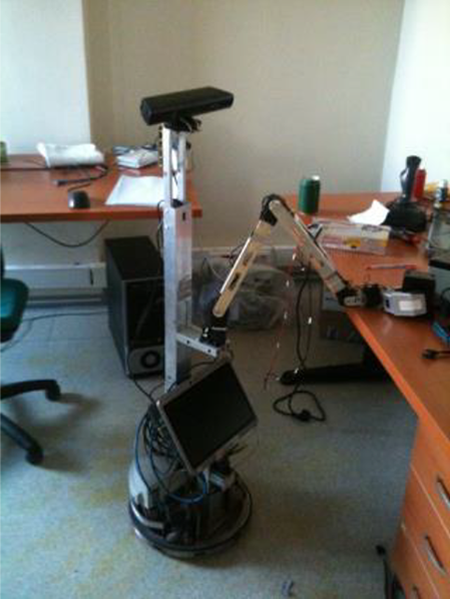
Robot platform used in experiments.

Figure 12.

Some examples from the dynamism in the environment between mapping and localization episodes.

different hours of day,

some curtains are closed,

some chairs are displaced,

occasional unexpected human obstruction, and

some tabletop objects.

The observations extracted with the methods described in “Camera feature” and “Laser feature” sections are compatible with the discrete models, for that reason, we tested our optimization method in a discrete localization setting. The robot is navigated manually with constant speed and each time the robot makes a displacement of 30 cm, a new place, representing the current position and observations is added to the list of places. Figure 13 illustrates the place creation process and shows the layout of the environment. The localization is performed among the places collected in the mapping episode. The first episode is used for training BoW clusters and associating to the places. The BoW algorithm is trained with 700 clusters, chosen empirically, and histograms are compared with the correlation method. The second episode is used for localization in the generated map. Each episode contains around 700 places. To gather the ground truth information, some control points are selected in both episodes that correspond to the same point in the real world. Given the constant speed of the robot, time span between the control points is interpolated to match the places in both episodes. The ground truth data are used in the calculation of the average position error of the localization algorithm. For each time step, the position index error is given by

\sum_{i} τ_{t, i} (i - g_{t})

Figure 13.

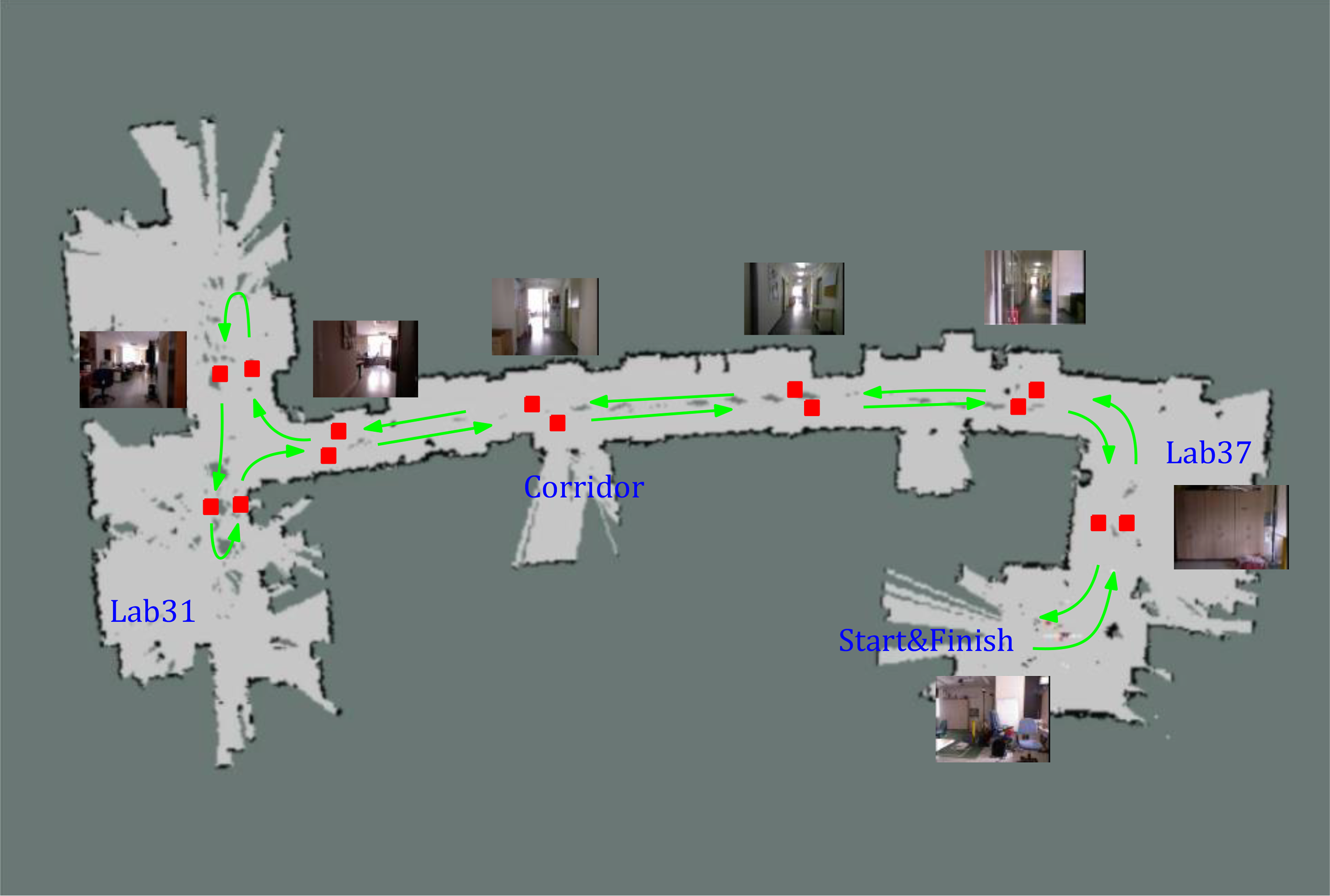
Illustration of map creation. Robot is navigated manually, new places (illustrated as red rectangles) are created at every 30 cm and associated with image (and laser) features. Note that the occupancy map is for illustration purposes and does not have an effect on the algorithm or results.

where $g_{t}$ is the index of the ground truth place for time t. The unit of the error is the edge count between places, which roughly translates to 30 cm.

There are two large labs and a corridor in the episodes. The regions are defined with the doorways being region boundaries. The robot passed two different doors four times, so there are five regions with transitions near time steps 80, 220, 460, and 600. The robot visited Lab 37, corridor, Lab 31, corridor, and finally Lab 37 again. To show that a single observation type may not be robust in all regions, we also excluded the effects of the localization algorithm and tested the observation model through regression with the K-NN algorithm. For each place in the localization episode, the average index of the most similar K places from the mapping episodes is illustrated in Figure 14(a) for image features and Figure 14(b) for laser features. While it is more pronounced for the image features, the distribution of the most likely place varies in different regions for both feature types.

Figure 14.

Observation qualities throughout the environment. Each point represents the most likely place association with the observation model. Diagonal layout is the true association. The regions are also illustrated.

The final weights obtained from the EM algorithm are reported in Table 3. Note that the weights agree with the results from Figure 14(a) that image features perform comparatively well in corridor, but poorly in the labs.

Table 3.

Weights for regions.

	Image	Laser
Lab 37	0.321	0.678
Corridor	0.886	0.113
Lab 31	0.501	0.498
Corridor	0.624	0.375
Lab 37	0.214	0.786

The comparison of trajectory errors of optimized weights with single feature types as well as equally weighted features is given in Table 4. The effect of using optimized weights in the localization episode can be seen more clearly in Figure 15. The boundaries of regions are also overlaid onto the position error plots. Note that the laser and image features perform poorly in different regions, but the weighted observation model keeps the error low.

Figure 15.

Trajectory error comparison for the localization episode. The unit of error is the mean position index difference.

Table 4.

Trajectory error comparison.

	Mean position index error
Image	9.113
Laser	12.201
Equal weights	7.388
EM weights	6.270

EM: expectation maximization.

Experiments on the COsy Localization Database data set

We also tested our method on the COsy Localization Database (COLD).³⁹ The data set includes raw sensory data from three different environments under various illumination conditions. Each environment includes data taken during cloudy weather, sunny weather, and at night. We chose two COLD-Freiburg subsets with cloudy and night conditions, because we want to introduce dynamism between the mapping and localization episodes. The episode with cloudy conditions is used as the mapping episode, and the night recording is used as the localization episode. Some of the properties of the data sets used are as follows:

robotic platform: ActivMedia Pioneer-3;

both omnidirectional and regular images;

laser range scans; and

Nine regions labeled with six different environment types.

The data are collected from the robot that is manually driven on a specific path in both episodes. Each episode took about 8 min with frequent stops. Our displacement-based place creation algorithm created 578 place in the mapping set and 562 place in the localization set. The data set includes about five frames per second camera images, each labeled with the current room type and the pose taken.

We extracted two feature types as discussed in “Camera feature” and “Laser feature” sections. The BoW algorithm is trained with 300 clusters, chosen empirically, and histograms are compared with the χ ² method. The maximum range of the laser range finder in the data set is clamped to 20 m.

The optimized weights for the regions is given in Table 5, and the comparison of trajectory errors for the localization episode is given in Table 6. Even though the optimized weights outperformed others, the decrease in trajectory error provided by the optimized weights is lower compared to the previous experiment in Table 4. This can be explained with the domination of image features in most of the regions, which is also reflected in the region weights in Table 5.

Table 5.

Weights for regions in COLD data set.

	Image	Laser
Reg 1	0.5911	0.4089
Reg 2	0.6801	0.3199
Reg 3	0.7722	0.2278
Reg 4	0.6224	0.3776
Reg 5	0.5059	0.4941
Reg 6	0.7340	0.2660
Reg 7	0.5852	0.4148
Reg 8	0.2934	0.7066
Reg 9	0.7328	0.2672

Reg: region; COLD: COsy Localization Database.

Table 6.

Regression errors in COLD database.

	Mean position index error
Image	12.650
Laser	14.817
Equal weights	12.821
EM weights	12.209

EM: expectation maximization; COLD: COsy Localization Database.

Conclusions

In this work, a feature type selection algorithm based on the local environment is developed for self-localization. The main contribution of this method is using more than one feature in a complementary way to increase overall robustness and localization accuracy. A latent variable about the quality of feature types is introduced to the observation model of the probabilistic localization problem, which is then estimated with a batch EM algorithm. The method is tested in the real world, simulations, and public COLD data set. The localization accuracy is compared with individual feature types and a naive fusion strategy. The data show that the optimized weights of feature types align with the changing qualities of the observations and making soft selections with those weights resulted with the best localization accuracy.

In this work, the feature qualities are estimated per local region, and regions in the environment are formed independently of features. As a future work, having a place classification strategy, such as in the work of Pronobis and Jensfelt,⁴⁰ would make the regions more aligned with the feature performance. Such change would also enable carrying of estimated weights to a new environment by associating new regions to the already experienced ones.

Footnotes

Declaration of conflicting interests

The author(s) declared no potential conflicts of interest with respect to the research, authorship, and/or publication of this article.

Funding

The author(s) disclosed receipt of following financial support for the research, authorship, and/or publication of this article: This work has been jointly supported by Bogazici University Scientific Research Fund project BAP13162 and Turkish State Planning Organization (DPT) under grant DPT 2007K120610.

ORCID iD

Nezih Ergin Özkucur

References

Leonard

Durrant-Whyte

. Mobile robot localization by tracking geometric beacons. IEEE Trans Robot Autom 1991; 7(3): 376–382.

Chen

McDonald-Maier

. Ekf based mobile robot localization. In: 2012 third international conference on emerging security technologies (EST), Lisbon, Portugal, 2012, pp. 149–154.

Dellaert

Fox

Burgard

. Monte Carlo localization for mobile robots. In: IEEE international conference on robotics and automation, Detroit, MI, USA, 10–15 May 1999, Vol. 2, pp. 1322–1328. IEEE.

Wolf

Burgard

Burkhardt

. Robust vision-based localization for mobile robots using an image retrieval system based on invariant features. In: IEEE international conference on robotics and automation (ICRA), 2002, Vol. 1, pp. 359–365.

Kuipers

Byun

. A robot exploration and mapping strategy based on a semantic hierarchy of spatial representations. J Robot Auton Syst 1991; 8: 47–63.

Badino

Huber

Kanade

. Real-time topometric localization. In: IEEE international conference on robotics and automation, Saint Paul, MN, USA, 14–18 May 2012, pp. 1635–1642. IEEE.

Kosecka

. Vision based topological Markov localization. In: IEEE international conference on robotics and automation (ICRA), New Orleans, LA, USA, 26 April–1 May 2004, Vol. 2, pp. 1481–1486. IEEE.

Thrun

. Robotic mapping: a survey. In: Lakemeyer

Nebel

(eds), Exploring artificial intelligence in the new millenium. San Francisco, CA, USA: Morgan Kaufmann Publishers Inc, 2002, pp. 1–35.

Milios

. Globally consistent range scan alignment for environment mapping. Auton Robot 1997; 4(4): 333–349.

10.

Grisetti

Stachniss

Burgard

. Improved techniques for grid mapping with rao-blackwellized particle filters. IEEE Trans Robot 2007; 23(1): 34–46.

11.

Burguera

Gonzalez

Oliver

. The likelihood field approach to sonar scan matching. In: IEEE/RSJ international conference on intelligent robots and systems, Nice, France, 22–26 September 2008, pp. 2977–2982. IEEE.

12.

Ravankar

Hoshino

. On a hopping-points SVD and Hough transform-based line detection algorithm for robot localization and mapping. Int J Adv Robot Syst 2016; 13(3): 98. DOI: 10.5772/63540.

13.

Libby

Kantor

. Deployment of a point and line feature localization system for an outdoor agriculture vehicle. In: IEEE international conference on robotics and automation (ICRA), Shanghai, China, 9–13 May 2011, pp. 1565–1570. IEEE.

14.

Lowe

. Distinctive image features from scale-invariant keypoints. Int J Comput Vision 2004; 60(2): 91–110.

15.

Lowe

Little

. Mobile robot localization and mapping with uncertainty using scale-invariant visual landmarks. Int J Robot Res 2002; 21(8): 735–758.

16.

Bay

Ess

Tuytelaars

. Speeded-up robust features (surf). Comput Vis Image Underst 2008; 110: 346–359.

17.

Wang

Fan

Qian

. Ego-motion estimation using sparse surf flow in monocular vision systems. Int J Adv Robot Syst 2016; 13(6): 1729881416671112.

18.

Werner

Sitte

Maire

. Visual topological mapping and localisation using colour histograms. In: 10th international conference on Control, automation, robotics and vision, ICARCV, Hanoi, Vietnam, 17–20 December 2008, pp. 341–346. IEEE.

19.

Csurka

Dance

Fan

. Visual categorization with bags of keypoints. In: Workshop on statistical learning in computer vision (eds Pajdla

Matas

), ECCV, Prague, Czech Republic, 11–14 May 2004, pp. 1–22. Springer.

20.

Erinc

Carpin

. Anytime merging of appearance-based maps. Auton Robot 2014; 36(3): 241–256.

21.

Philbin

Chum

Isard

. Object retrieval with large vocabularies and fast spatial matching. In: IEEE conference on computer vision and pattern recognition, Minneapolis, MN, USA, 17–22 June 2007, pp. 1–8. IEEE.

22.

Cummins

Newman

. Appearance-only slam at large scale with FAB-MAP 2.0. Int J Robot Res 2011; 30(9): 1100–1123.

23.

Milford

Wyeth

. SeqSLAM: Visual route-based navigation for sunny summer days and stormy winter nights. In: IEEE international conference on robotics and automation, Saint Paul, MN, USA, 14–18 May 2012, pp. 1643–1649. IEEE.

24.

Durrant-Whyte

. Sensor models and multisensor integration. Int J Robot Res 1988; 7(6): 97–113.

25.

Castellanos

Neira

Tardós

. Multisensor fusion for simultaneous localization and map building. IEEE Trans Robot Autom 2001; 17(6): 908–914.

26.

Deelertpaiboon

Parnichkun

. Fusion of GPS, compass, and camera for localization of an intelligent vehicle. Int J Adv Robot Syst 2008; 5(4): 46.

27.

Zhu

Leung

. Recursive variational Bayesian inference to simultaneous registration and fusion. Int J Adv Robot Syst 2016; 13(3): 124.

28.

Caron

Davy

Duflos

. Particle filtering for multisensor data fusion with switching observation models: application to land vehicle positioning. IEEE Trans Signal Proc 2007; 55(6–1): 2703–2719.

29.

Dempster

Laird

Rubin

. Maximum likelihood from incomplete data via the EM algorithm. J Royal Stat Soc Ser B 1977; 39(1): 1–38.

30.

Burgard

Fox

Jans

. Sonar-based mapping with mobile robots using EM. In: Proceeding of 16th international conference on machine learning (eds Bratko

Dzeroski

), Bled, Slovenia, 27–30 June 1999, pp. 67–76. San Francisco, CA, USA: Morgan Kaufmann Publishers Inc.

31.

Lee

Fraundorfer

Pollefeys

. Robust pose-graph loop-closures with expectation-maximization. In: IEEE/RSJ international conference on intelligent robots and systems, Tokyo, Japan, 3–7 November 2013, pp. 556–563. IEEE.

32.

Rogers

Trevor

AJB

Nieto-Granda

. SLAM with expectation maximization for moveable object tracking. In: IROS, IEEE, Taipei, Taiwan, 18–22 October 2010, pp. 2077–2082. IEEE.

33.

Thrun

Burgard

Fox

. Probabilistic robotics. Cambridge, MA: MIT Press, 2005.

34.

Liu

. Monte Carlo strategies in scientific computing. New York, NY, USA: Springer Publishing Company, Incorporated, 2008. ISBN: 0387763694, 9780387763699.

35.

Beyer

. The theory of evolution strategies. Heidelberg Berlin: Springer-Verlag, 2001.

36.

Fischler

Bolles

. Random sample consensus: a paradigm for model fitting with applications to image analysis and automated cartography. Commun ACM 1981; 24(6): 381–395.

37.

ElKaissi

Elgamel

Bayoumi

. SEDLRF: a new door detection system for topological maps. In: Proceedings of the IEEE international conference on application-specific systems, architectures and processors (ASAP), Montreal, Que., Canada, 18–20 August 2006. IEEE.

38.

Festo robotino. https://www.festo-didactic.com/int-en/learning-systems/education-and-research-robots-robotino/ (2007, accessed 24 November 2018).

39.

Pronobis

Caputo

COLD: COsy Localization Database. Int J Robot Res 2009; 28(5): 588–594.

40.

Pronobis

Jensfelt

. Large-scale semantic mapping and reasoning with heterogeneous modalities. In: IEEE international conference on robotics and automation (ICRA), Saint Paul, MN, USA, 14–18 May 2012, pp. 3515–3522. IEEE.

Autonomous feature type selection based on environment using expectation maximization in self-localization

Abstract

Keywords

Introduction

Proposed approach

Basic localization model

Multiple feature types

Optimization with EM

Application to MCL

Real-world features

Camera features

Laser features

Region change detection

Experiments and results

Simulation experiment with particle filters

Real-world experiments

Experiments on the COsy Localization Database data set

Conclusions

Footnotes

Declaration of conflicting interests

Funding

ORCID iD

References