Sage Journals: Discover world-class research

Abstract

Propellers are one of the key parts on the autonomous underwater vehicles. When adopting the conventional particle filter to estimate the degree of fault, based on the status given by the sensors, the diagnosis value is not always satisfactory in the transition stage (as it accelerates substantially). The diagnosis value is relatively larger than it is in the cruising stage, and this might weaken the ability to classify using the fault diagnosis method. This article proposes a new fault diagnosis method combining the grey prediction and rank particle filter method. The main improvements include two aspects: status input prediction and thrust loss trend analysis. The status input into the rank particle filter is predicted by the grey prediction method, to meet the condition that the thrust loss estimation does not change quickly when the control signal changes drastically. Subsequently, the control signal change rate is combined to analyse the thrust loss change trend. This improvement reduces the diagnosis value under normal conditions and enlarges the ratio between faulty and normal conditions. Simulation experiments are carried out to verify the performance of the proposed algorithm. The results show that the proposed method could reduce the thrust loss estimation error and enlarge the ratio of diagnosis value between faulty and normal conditions, providing basis for the following operation.

Keywords

Autonomous underwater vehicle status estimation fault diagnosis grey prediction particle filter

Introduction

Autonomous underwater vehicles (AUVs) play a significant role in the exploration of oceans, owing to their manoeuvrability and long-range survey. However, the underwater environment is complex and variable, so they may face harsh conditions in some circumstances. This environmental uncertainty may cause varying degrees of affection on the AUVs, including the propellers. Faults in the propeller may influence the completion of tasks and even cause damages on the AUVs, when the propeller cannot output the desired thrust. Therefore, now there is increased attention for detecting underlying faults, while an AUV is working autonomously.

With the help of sensors, the AUV’s fault is diagnosed through the analysis of its status; for example, Abed et al.¹ analysed the vibration and current signals to derive fault severity prediction regarding damage of the blades and Filaretov et al.² applied data fusion on AUV fault detection and localization. Chu and Zhang³ reconstructed the fault with the help of a terminal sliding observer. Raanan et al.⁴ applied an online Bayesian nonparametric topic modelling technique to AUV sensor data to characterize its performance patterns automatically, while Xiang et al.⁵ chose to use neural networks to combine the faults together in different AUV subsystems. Besides, status estimation methods such as particle filter also attract the interest of fault diagnosis researchers because of its accuracy and ease of use; for instance, Barisic et al.⁶ presented research about an implementation of the sigma-point unscented Kalman filter and Zhao et al.⁷ applied the particle filter-based fault diagnosis method to detect propeller faults in an underwater robot. Daroogheh et al.⁸ proposed a dual estimation methodology in particle filtering for both time-varying parameters and states, and Sun et al.⁹ used the Gaussian particle filter to estimate the thrust loss in order to detect the fault in an AUV.

When we applied the conventional thrust loss estimation method, using a particle filter⁹ to detect the fault of an AUV, we found that the fault diagnosis algorithm gave a larger diagnosis value in the transition stage (when the AUV is accelerating substantially) than in the cruising stage. We analysed this phenomenon and concluded that this may be due to the fact that the conventional algorithm did not consider the influence of the control signal change. The thrust loss estimation could not change instantly, when the control signal exhibits a higher change rate. The control signals stated above are the instructions that will be dealt with the force allocation algorithm and calculated as the voltage input of the propellers. Therefore, the change of the control signal can be treated as the change of control force or propeller thrust desired change. Since a larger diagnostic value in the transition stage could lead to a smaller diagnosis value ratio of faulty conditions to normal conditions, this may lead to misdiagnosis or increase the difficulty to determine the threshold.

Based on the consideration above, an improved fault diagnosis method has been proposed. To be specific, two aspects were proposed, including reducing the estimation error of the thrust loss (with the help of AUV state grey prediction), like the method¹⁰ proposed that including information from the predicted future trials to achieve a better performance; and the influence of control signals’ variation was considered while analysing the thrust loss.

This article has been organized as follows. In “AUV mathematical model and faulty model” section, we have established the mathematical model of AUV and introduced the basic fault estimation concept. Then, “Basic grey prediction and the improved algorithm” section describes the conventional grey prediction model and its improvement. “Basic rank sampling method and rank particle filter” section describes the rank particle filter built on the rank sampling method. “Improved AUV propeller fault diagnosis method” section combines the improved grey prediction method with the rank particle filter, proposing the grey prediction rank particle filter (GP-RPF) fault diagnosis method. Experimental simulations are shown in ‘Fault diagnosis simulations’ section, and we have drawn our conclusions in the last section.

AUV mathematical model and faulty model

The proposed method needed the thrust loss estimated by the AUV mathematical model to detect the fault. Therefore, a torpedo type of AUV, with no fins or wings, was selected as the object of the study, and on which the control force was provided by its propellers.

Firstly, the space coordinate system was defined by the International Ship Model Towel Pool Recall and the Shipbuilding and Engineering Society terminology bulletin system, as shown in Figure 1.

Figure 1.

Three stages of AUV underwater mobile recovery. AUV: autonomous underwater vehicle.

The E − ξηζ geodetic coordinate system was fixed on earth, and the origin of the body coordinate system O − xyz was fixed at the AUV’s centre of gravity. The AUV’s mathematical model was decomposed subsequently, and the focus was mainly on the motion in the horizontal plane. In the horizontal plane, the motion of the AUV was controlled by two stern propellers, each of which was set to form a 13° angle with the longitudinal axis of the AUV, respectively, providing the thrust and yaw moment. In the horizontal plane, the body coordinate system and the geodetic coordinate system had the corresponding relations as mentioned below

[\begin{matrix} x \\ y \\ z \end{matrix}] = T^{- 1} [\begin{matrix} ξ \\ η \\ ζ \end{matrix}]

where

Τ^{- 1} = [\begin{matrix} cos ψ cos θ & sin ψ cos θ & - sin θ \\ cos ψ sin θ sin ϕ - sin ψ cos ϕ & sin ψ sin θ sin ϕ + cos ψ cos ϕ & cos θ sin ϕ \\ cos ψ sin θ cos ϕ + sin ψ sin ϕ & sin ψ sin θ cos ϕ - cos ψ sin ϕ & cos θ cos ϕ \end{matrix}]

where ϕ is the roll angle and tilting to the right is positive, θ is the pitch angle and tilting to the stern is positive and ψ is the yaw angle and turning to the right is positive.

We assumed that the AUV sailed in a deep and still environment and the wave force was excluded. The force exerted on the AUV was provided solely by the hydrodynamic force and the propeller thrust

D \dot{X} = F_{vis} + F_{propeller}

D is the AUV hydrodynamic parameters matrix, X is the status of the AUV, F_vis is the non-inertial hydrodynamic term, while F_propeller is the propeller thrust.

Based on the assumption above, the state space equation of the AUV could be achieved. The motion system of the AUV was highly nonlinear, and the continuous equation could be discretized as the following discrete state space equations

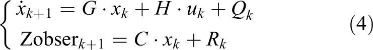
{\begin{cases} {\dot{x}}_{k + 1} = G \cdot x_{k} + H \cdot u_{k} + Q_{k} \\ {Zobser}_{k + 1} = C \cdot x_{k} + R_{k} \end{cases}

where G is the system matrix, x_k is the vector of the state variables at time k, u_k is the control input, H is the system input matrix, Zobser_k is the observer value, C is the observation matrix and Q_k and R_k are the process noise and measurement noise, respectively.

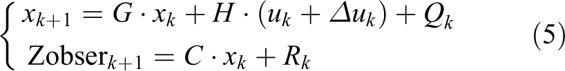
We knew that the propeller fault would restrict the output thrust to some degree. Therefore, the actual control force exerted on the AUV would change at faulty condition. To elaborate, the actual control force at time k will deviate from u_k to u_k + Δ u_k, where Δu_k should be near zero when the propeller was fault-free. The AUV’s fault in the propeller could be estimated using the faulty mathematical model of the AUV, as shown below

{\begin{cases} x_{k + 1} = G \cdot x_{k} + H \cdot (u_{k} + Δ u_{k}) + Q_{k} \\ {Zobser}_{k + 1} = C \cdot x_{k} + R_{k} \end{cases}

Basic grey prediction and the improved algorithm

The grey model has been widely used in terms of small sample prediction, and the prediction results have been universally accepted in time series data. We primarily focused on the GM(1,1) model here, and its prediction procedure could be summarized as follows:

selecting the original data sequences;

applying accumulated generating operation (AGO) to the selected data sequences;

the accumulated generated sequences constructing the grey background values;

building GM(1,1) model based on the grey background values;

obtaining the solutions of the Whiting differential equations; and

applying inverse AGO to generate predicted sequences.

The conventional grey prediction method could get acceptable prediction errors in most cases. However, the errors may lead to bigger diagnosis errors in the next step, taking the nonlinear relationship into consideration, between the AUV state and the exerted control force. Liu et al.¹¹ prompted an improved GM(1,1) to the point that the conventional grey model prediction error was not always satisfactory. The proposed GM(1,1) improved the construction of the grey background value and the solution of the Whiting differential equation.

In the aspect of construction of grey background value

Z^{(1)} (k) = \int_{k - 1}^{k} X^{(1)} (t) d t

where X⁽¹⁾(t) is the accumulated generation sequence and Z⁽¹⁾(t) is the grey background value.

In the conventional method, as Zhou and Zhu did,¹² the grey background value was approximated based on

Z^{(1)} (k) = \frac{1}{2} [X^{(1)} (k) + X^{(1)} (k - 1)]

However, Liu et al. used a nonlinear operation to obtain the result

Z^{(1)} (k) = \frac{X^{(1)} (k) - X^{(1)} (k - 1)}{ln X^{(1)} (k) - ln X^{(1)} (k - 1)}

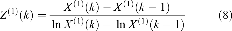
thereby eliminating the error between practical and approximation grey background values.

In the solution of Whiting differential equation method, it was different from the conventional grey prediction method, where the initial point of the original sequence was selected as the initial condition. Liu et al. selected a special point as the solution, which was best approximated in the prediction index. It is shown as

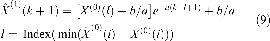
\begin{array}{l} {\hat{X}}^{(1)} (k + 1) = [X^{(0)} (l) - b / a] e^{- a (k - l + 1)} + b / a \\ l = Index (min ({\hat{X}}^{(0)} (i) - X^{(0)} (i))) \end{array}

X⁽⁰⁾(l) is the selected special point; the second equation was to find the best approximated value in the prediction index; a and b are grey development coefficient and grey action quantity respectively ${\hat{X}}^{(0)} (i)$ and X⁽⁰⁾(i) are the predicted value sequence and real value sequence, respectively.

Based on the improvements mentioned above, in the conventional grey prediction method, a better performance in prediction error indexes was obtained, which formed the fundamental for the next step.

Basic rank sampling method and rank particle filter

The rank filtering method¹³ was prompted from the rank sampling method, where the importance density function provided was in line with the probability density of the truth state. Fu et al.¹⁴ combined the advantages of the rank filtering method and particle filter method to present the rank particle filter.

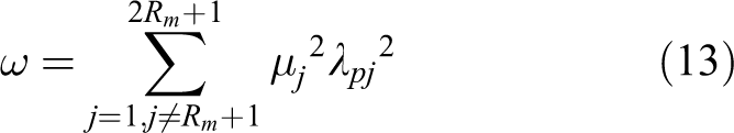
The rank sampling method was a deterministic sampling method. First, we determined the state vector X with a mean value $\bar{X}$ and the covariance matrix Cov_x and then calculated the mean and mean square error of the nonlinear change f(X).

According to $\bar{X}$ and Cov_x, the initial sample points x SigmaPts were obtained

x SigmaPts (i) = \bar{X} + μ_{j} λ_{p j} {(\sqrt{{Cov}_{X}})}_{l}

where l = 1, 2, ..., R_n (R_n is the dimension of X) and i = (j − 1)R_n + 1. λ _pj is the lower bound of the confidence interval with probability and p_j is the X distribution. μ_j is the correction factor of the sampling point.

The initial sampling points were subject to nonlinear changes to obtain the set of output variables x Pred:

x Pred (i) = f (x SigmaPts (i))

Then, the mean and covariance of the output variables were calculated

\begin{array}{l} \bar{x Pred} = \frac{1}{n Pts} \sum_{i = 1}^{n Pts} x Pred (i) \\ {Cov}_{x Pred} = \frac{1}{ω} \sum_{i = 1}^{n Pts} μ_{i} (x Pred (i) - \bar{x Pred}) {(x Pred (i) - \bar{x Pred})}^{T} \end{array}

The weight coefficient of the covariance is ω

ω = \sum_{j = 1, j \neq R_{m} + 1}^{2 R_{m} + 1} μ_{j}^{2} λ_{p j}^{2}

We now know that x SigmaPts was the initial sample point from the posterior probability distribution $N (\bar{X}, {Cov}_{x})$ , and it was updated to generate x Pred and corresponding weights via the rank filter method mentioned above. Further, we assumed that x Pred(k, i) was one of the sampling points in x Pred(k) at time k obtained by the particle filter sampling process. The discrete distribution could be obtained, containing the sample points and weights ω(k, i)

\hat{p} (x Pred (k) | {Zobser}_{0 : k}) = \sum_{i = 1}^{N} ω (k, i) δ (x Pred (k) - x Pred (k | k - 1, i))

where δ(x) is the Dirac delta function.

In the next step, the new particle set could be obtained from the distribution, as well as the important weights. This was the same process to go through, as the conventional particle filter. The basic rank particle filter method was thus established. With the help of the rank particle filter, we could estimate the thrust loss, so as to detect the fault in the AUV.

Improved AUV propeller fault diagnosis method

With the faulty mathematical model of the AUV, the original rank particle filter was constructed in the last section, according to the thrust loss estimation method⁹ prompted in 2016

{\begin{cases} x_{k + 1} = G \cdot x_{k} + H \cdot (u_{k} + Δ u_{k}) + Q_{k} \\ {Zobser}_{k + 1} = C \cdot x_{k} + R_{k} \end{cases}

where $Δ u_{k} = (Δ X, Δ Y, Δ Z, Δ K, Δ M, Δ N)$ .

As shown in Figure 2, the key of the conventional fault diagnosis method mentioned above was to analyse the value Δu_k and its trend, which should be near zero in the normal state. When fault emerged at one of the propellers, the thrust loss Δu_k changed in some degree, whose amplitude was affected by the severity of the fault. The thrust loss trend was then analysed by the modified Bayes (MB) algorithm, and the predefined threshold was used to detect whether a fault occurred in the propeller. Therefore, the thrust estimation accuracy and analysing its trend properly play an important role here.

Figure 2.

Conventional fault diagnosis method.

A torpedo-shaped AUV had the benefit of reducing the flow resistance. This type of AUV was appropriate for search missions in a vast region, compared to the frame-shaped AUV, which was appropriate for manipulation tasks. Moving along a straight line was the most common action of these torpedo-shaped AUVs.¹⁵ When this conventional method was used to estimate the thrust loss of the AUV, it was found that the fault diagnosis algorithm performed better in the cruising stage, compared to the transition stage. This was because when control signal experienced a great change rate, the thrust estimation could not change instantly. This influence was small during the steady cruising stage, with small status changes. But the influence in the transition stage was more severe, leading to a bigger estimation error.

Considering the problem above, we improved the conventional method, combining the grey prediction method. The grey prediction method was not introduced for the first time into the particle filter. For example, Chen et al.¹⁶ used a group of grey prediction particles to predict status updating, and the rest of the particles updated by the state space equations. This was different from our proposed method. According to Figure 3, we used the grey prediction method to predict the AUV status, and the predicted status was combined with the control signals as the input of the rank particle filter.

Figure 3.

Proposed fault diagnosis method.

Meanwhile, in Figure 2, the MB algorithm was used to analyse the time range for the AUV to attain thrust loss. When the diagnosis value was beyond the threshold, a fault was detected by the algorithm. However, in the conventional algorithm, only the thrust loss was selected as the input of the algorithm, ignoring the influence of the control signal change. We found that this method could be improved to some extent: The thrust loss estimated had to be considered along with the amplitude of the control signal change. We defined the CT(k) as the diagnosis value at time k combined with the control signal and the rate of thrust loss, thereby improving it from the conventional analysis method.

The diagnosis value CT(k) is defined as follow

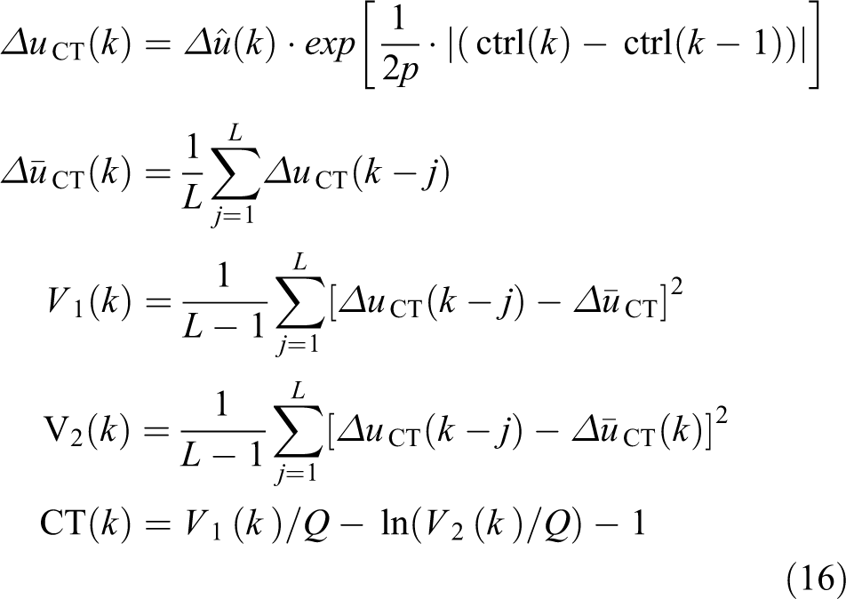
\begin{array}{l} Δ u_{CT} (k) = Δ \hat{u} (k) \cdot e x p [\frac{1}{2 p} \cdot | (ctrl (k) - ctrl (k - 1)) |] \\ Δ {\bar{u}}_{CT} (k) = \frac{1}{L} \sum_{j = 1}^{L} Δ u_{CT} (k - j) \\ V_{1} (k) = \frac{1}{L - 1} \sum_{j = 1}^{L} {[Δ u_{CT} (k - j) - Δ {\bar{u}}_{CT}]}^{2} \\ V_{2} (k) = \frac{1}{L - 1} \sum_{j = 1}^{L} {[Δ u_{CT} (k - j) - Δ {\bar{u}}_{CT} (k)]}^{2} \\ CT (k) = V_{1} (k)/ Q - ln (V_{2} (k)/ Q) - 1 \end{array}

where Δu_CT was the thrust loss estimation combined with control signals; ctrl(k) and ctrl(k-1) were the control signals at time k and k-1, respectively; and p was the parameter subject to the normal control signal change rate. The mean value $Δ {\bar{u}}_{CT}$ and the variance V(k) of the analysing points were obtained subsequently, and the points were selected as the recent L status points autonomously. Finally, the diagnosis value CT(k) was marked as the fault degree

Fault diagnosis simulations

During the test with this type of AUV, it was found that a faulty propeller might not output enough thrust always. When the desired thrust was small, the propeller could output the required thrust normally; however, when the desired thrust was greater than a certain value, the propeller could not reach the desired output thrust.

To show the effect of control force on the estimation of thrust loss in the transition stage, a simulation of AUV accelerating to the desired velocity from the halted state was generated. In the first 50 s, the desired velocity was set as 0.5 m/s and from 50 s to 100 s, the desired velocity was set as 1.0 m/s.

Figures 4 and 5 show the simulation experiment results. The blue line is the conventional estimation result and the red line is the proposed algorithm’s estimation result. It can be seen in Figure 5 that the estimated thrust loss in the transition stage gave a bigger value than at other times, which might lead to a misdiagnosis of the propeller. In ideal conditions, the thrust loss in the X-axis should be zero, in the condition without fault. We calculated the root mean square error (RMSE) of the thrust loss estimation in the X-axis and the values obtained were 86.16 using the conventional method and 59.55 using the proposed method, reducing it by about 30%.

Figure 4.

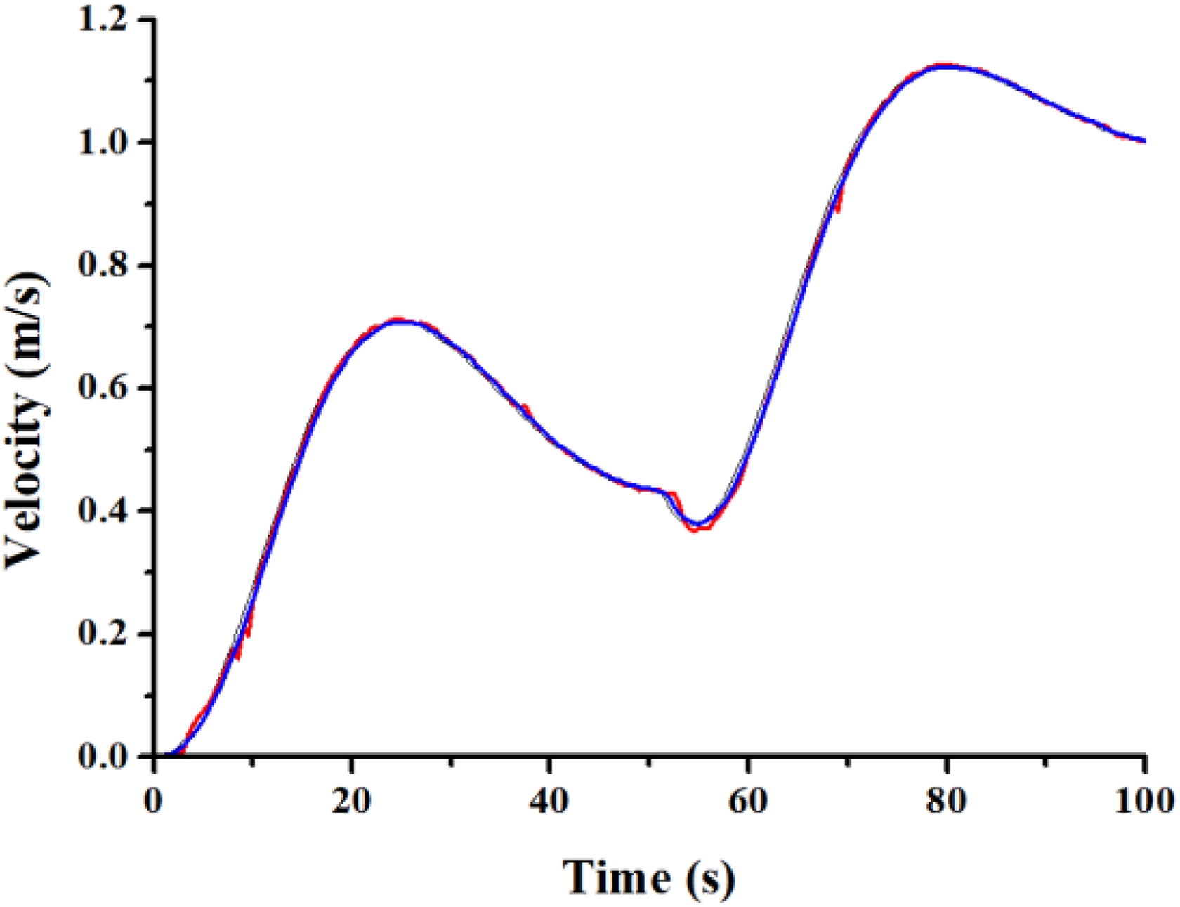
AUV velocity curve. AUV: autonomous underwater vehicle.

Figure 5.

Estimation thrust loss in X-axis.

Although in this work process of AUV, there was no fault occurrence, the control force’s change substantially led to a bigger estimation of thrust loss in this stage. This was analysed by the algorithm as a potential cause for misdiagnosis. After combining the improved fault diagnosis method, the diagnosis value results were shown in Figure 6. We calculated the RMSE of the diagnosis value and it was 63.32 using the conventional method and 42.32 using the proposed method, reducing it by about 33%. From the comparison between the proposed and conventional algorithm, we could find that the proposed algorithm gave a better diagnosis value of the AUV state. This would pave the way for a better diagnosis value.

Figure 6.

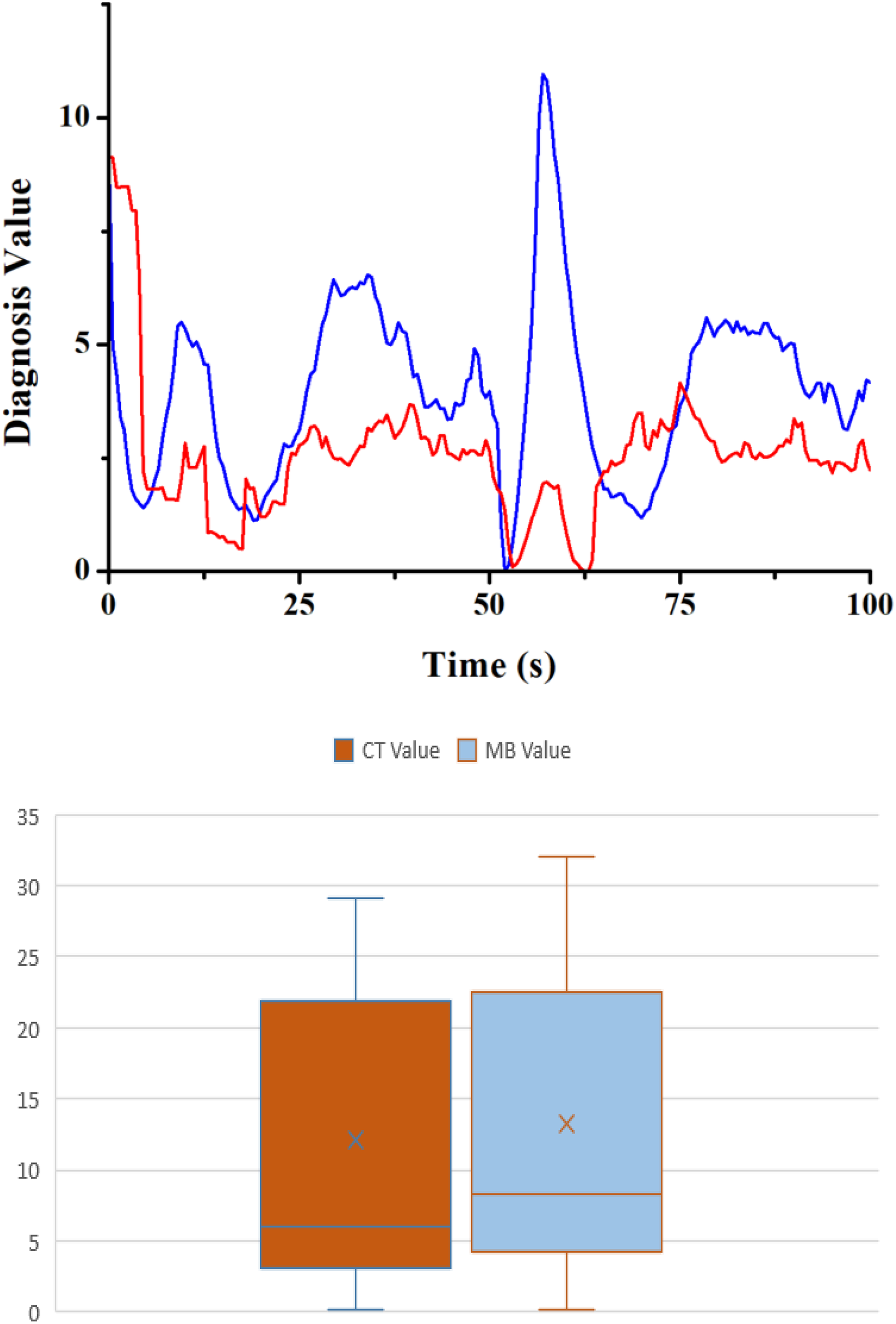
Diagnosis value comparison.

The next simulation condition was set as follows. In the first 50 s, the AUV was in a condition, wherein no fault occurred in the propeller. And after 50 s, there was a fault in the left propeller of the AUV, and it could only output 20 N, when the desired output was beyond 20 N, shown in Figure 7.

Figure 7.

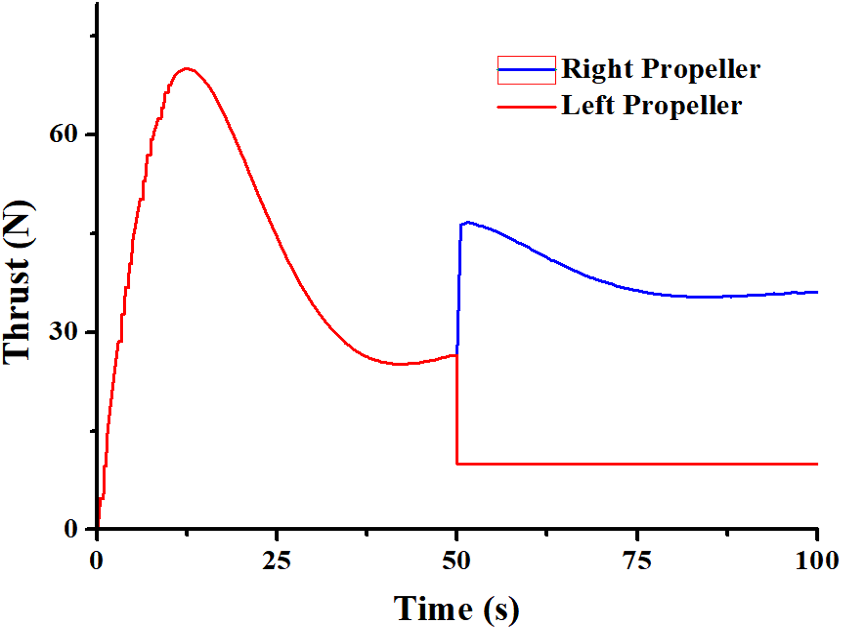
Thrust output by the propellers.

From the comparison in Figure 8, we could find that both the algorithms gave a relatively large value after 50 s, which was the time when a fault was induced. Because the fault was induced from 50 s, we considered the first 50 s from the beginning as the normal condition and the last 50 s as the fault condition. To compare the performance of the two algorithms, we calculated the mean value estimated by both the methods. The mean value in the normal condition given by the conventional method was 5.07 and the mean value in the faulty condition was 21.37. Meanwhile, the mean value in the normal condition given by the proposed method was 3.81, while the mean value in the faulty condition was 20.19. The diagnosis values in the fault condition given by both the algorithms were close, but the values in the normal condition in the proposed method were smaller. The ratio of the faulty to normal conditions given by the two algorithms was 4.22 and 5.29, respectively. The higher ratio gave more leeway for defining the threshold compared to other analysing methods in the fault identity step.

Figure 8.

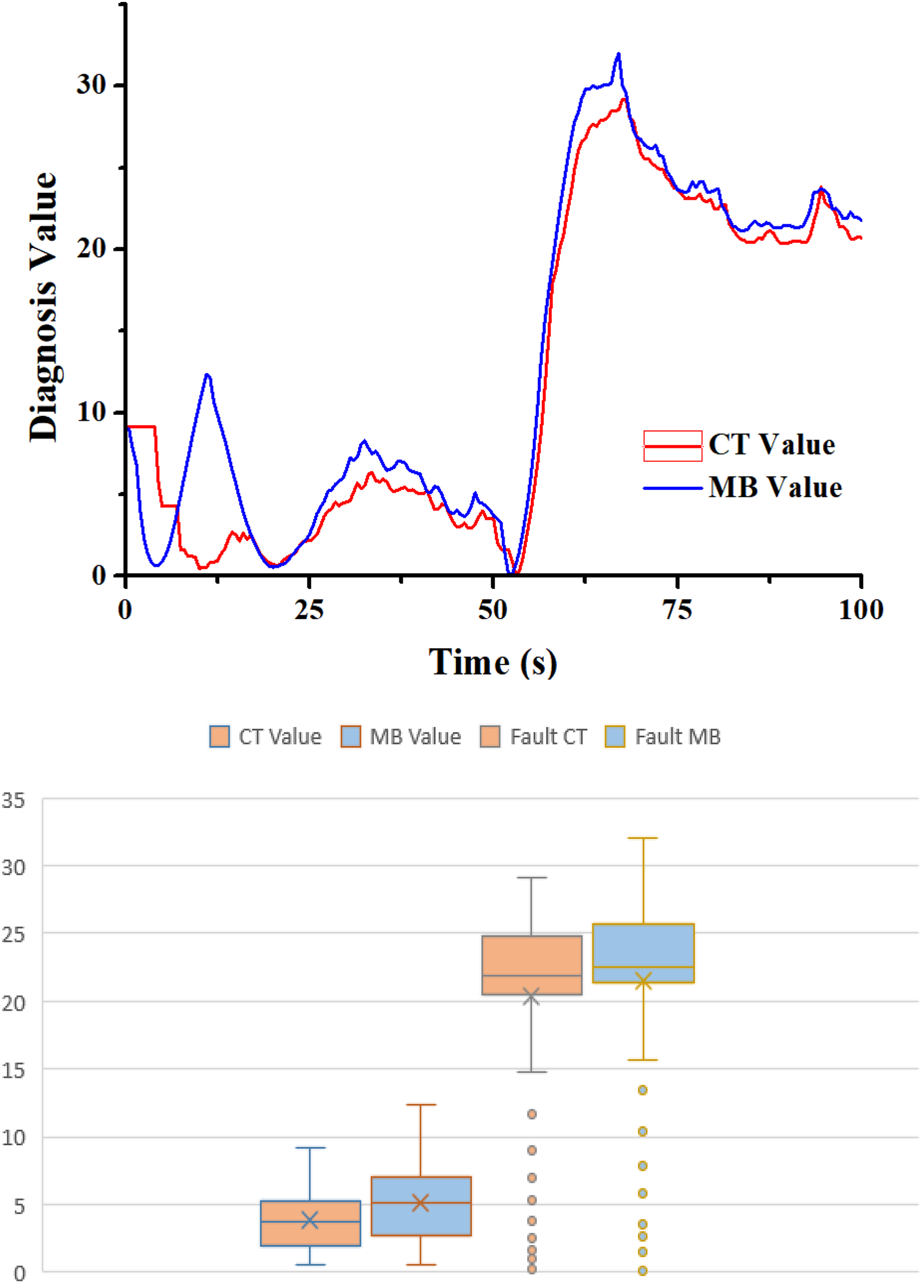
Diagnosis value given by the algorithms.

The situation above was when no fault occurred in the propeller during the transition stage. A condition to include fault occurrence was then set at the beginning. The fault condition was set in Figure 9 as follows: When the desired thrust provided by the left propeller was less than 30 N, the thrust was produced normally. However, when the value of the desired thrust was beyond 30 N, the propeller could not produce the requisite thrust, and it could only produce a thrust amounting to 30 N.

Figure 9.

Thrust output by the propellers.

From the comparison in Figure 10, it was found that although there was a delay in the proposed method to detect the fault, both the algorithms gave a high diagnosis value when compared to the normal condition. Since the grey prediction method needed a series of data to predict the status at the beginning of the time series, the proposed method gave a higher diagnosis value, and the ratio of the faulty to normal condition was 5.02, while the conventional method provided a result of 9.7. However, if we discarded the data at the beginning, the ratio of the proposed method rose to 10.92, and the conventional method descended to 10.05. Therefore, although there was a delay when the fault occurred at the beginning, the proposed method still could give an acceptable result.

Figure 10.

Diagnosis value given by the algorithms.

In the turning motion stage, the turning motion was controlled by only one of the stern propellers initially. For example, when the AUV turned to the left, the right propeller was primarily providing the thrust, and when a fault occurred in the left propeller, both the conventional and proposed method could not diagnose the fault. If the fault occurred in the right propeller, the phenomenon resembled a straight motion, as mentioned previously.

Finally, we used the proposed algorithm on a series of sea trial experiment data: the AUV started accelerating to 1.0 m/s to cruise along the predefined path, and a fault occurred in the propeller towards the end of the task, after which the AUV was recovered by us, as shown in Figure 11.

Figure 11.

AUV velocity in the sea trial. AUV: autonomous underwater vehicle.

From the comparison in Figure 12 between the results from the conventional and proposed methods, we could find that from the time stamp of 45–70 s, the AUV was accelerating and the diagnosis value given by the conventional and proposed algorithm gave a high diagnosis value, compared to the normal cruise condition. The diagnosis value CT(k) in the entire time zone was relatively smaller than the MB value. However, the ratio of the faulty condition to normal condition was larger than the MB value. The ratio of the faulty to normal condition given by the two algorithms was 6.97 and 10.47, respectively, enlarging the ratio by about 50.3%. This larger ratio gave more leeway to define the threshold of the faulty condition. Because the proposed method combined the control signal change, if we selected the maximum value in the normal condition as the threshold, the fault detected would be delayed by about 3 s. The AUV in water does not need quick manoeuvrability like unmanned aeroplanes, and therefore this delay is acceptable.

Figure 12.

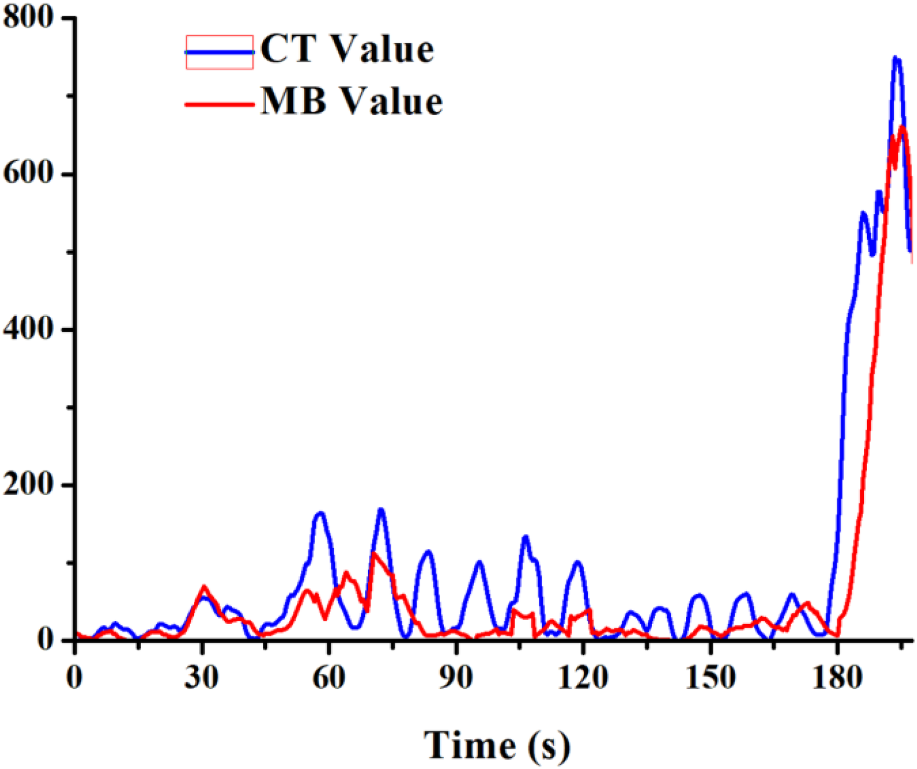
Diagnosis value given by the algorithms.

Conclusions

In the proposed method, we proposed a new fault diagnosis method combining the grey prediction method to improve the estimation accuracy of the AUV status and the thrust loss trend analysis method to combine the influence of the control signals. The simulation results pointed out that the proposed method could estimate the AUV status better and gave a larger ratio of the faulty to normal conditions than the conventional method, which could provide basis for fault identity in the next step.

Footnotes

Declaration of conflicting interests

The author(s) declared no potential conflicts of interest with respect to the research, authorship, and/or publication of this article.

Funding

The author(s) disclosed receipt of the following financial support for the research, authorship, and/or publication of this article: This work was supported by National Key R&D Program of China (2017YFC0305700), National Natural Science Foundation of China (51879057, 51809064), the China Postdoctoral Science Foundation (2017M621250) and the Fundamental Research Funds for the Central Universities (HEUCFG201810).

ORCID iD

Ye Li

Yanqing Jiang

References

Abed

Polvara

Singh

. Advanced feature extraction and dimensionality reduction for unmanned underwater vehicle fault diagnosis. In: UKACC 11th international conference on control, Belfast, 2016, pp. 1–6. DOI: 10.1109/CONTROL.2016.7737596.

Filaretov

Zhirabok

Zyev

. Design and investigation of dead reckoning system with accommodation to sensors errors for autonomous underwater vehicle. In: Oceans - MTS/IEEE Washington, Washington, DC, 2015, pp. 1–4. DOI: 10.23919/OCEANS.2015.7401832.

Chu

Zhang

. Fault reconstruction of thruster for autonomous underwater vehicle based on terminal sliding mode observer. Ocean Eng 2014; 88: 426–434.

Raanan

Bellingham

Zhang

. Detection of unanticipated faults for autonomous underwater vehicles using online topic models. J Field Robot 2017; 35: 705–716.

Xiang

Zhang

. On intelligent risk analysis and critical decision of underwater robotic vehicle. Ocean Eng 2017; 140: 453–465.

Barisic

Vasilijevic

Nad

. Sigma-point unscented kalman filter used for AUV navigation. In: 20th mediterranean conference on control and automation (MED), Barcelona, 2012, pp. 1365–1372. DOI: 10.1109/MED.2012.6265829.

Zhao

Skjetne

Blanke

. Particle filter for fault diagnosis and robust navigation of underwater robot. IEEE Trans Control Syst Technol 2014; 22: 2399–2407.

Daroogheh

Meskin

Khorasani

. A dual particle filter-based fault diagnosis scheme for nonlinear systems. In: IEEE transactions on control systems technology, Vol. 26, July 2018, pp. 1317–1334. DOI: 10.1109/TCST.2017.2705056.

Sun

Ran

. Thruster fault diagnosis method based on Gaussian particle filter for autonomous underwater vehicles. Int J Nav Arch Ocean 2016; 8: 243–251.

10.

Chu

Owens

Freeman

. Iterative learning control with predictive trial information: convergence, robustness, and experimental verification. IEEE Trans Control Syst Technol 2016; 24: 1101–1108.

11.

Liu

Zhang

Wang

. Weak thruster fault prediction method for autonomous underwater vehicle based on grey model. In: Proceedings of IMechE Part 1: J systems and control engineering, Shanghai, China, 10–13 April 2016. IEEE. DOI: 10.1177/0959651818793730.

12.

Zhou

Zhu

. A sensor fault diagnosis method for underwater vehicles based on GM(1,1). Shipbuilding of China 2011; 52: 137–144. DOI: 10.3969/j.issn.1000-4882.2011.01.017 (in Chinese).

13.

Xiao

. Rank filter method. J of Mech Streng 2014; 36: 521–526. DOI: 10.16579/j.issn.1001.9669.2014.04.031 (in Chinese).

14.

Xiao

Lou

. Rank particle filter. J Mech Streng 2014; 36: 894–898. DOI: 10.16579/j.issn.1001.9669.2014.06.031 (in Chinese).

15.

Farrell

Pang

. Biologically inspired chemical plume tracing on an autonomous underwater vehicle. In: IEEE international conference on systems, man and cybernetics (IEEE Cat. No.04CH37583), The Hague, 2004, Vol. 7, pp. 5991–5996. DOI: 10.1109/ICSMC.2004.1401337.

16.

Chen

Shi

Hong

. Grey prediction based particle filter for maneuvering target tracking. Prog Electromagn Res 2009; 93: 237–254.

Fault diagnosis in autonomous underwater vehicle propeller in the transition stage based on GP-RPF

Abstract

Keywords

Introduction

AUV mathematical model and faulty model

Basic grey prediction and the improved algorithm

Basic rank sampling method and rank particle filter

Improved AUV propeller fault diagnosis method

Fault diagnosis simulations

Conclusions

Footnotes

Declaration of conflicting interests

Funding

ORCID iD

References