Route optimizing and following for autonomous underwater vehicle ladder surveys

Abstract

An autonomous underwater vehicle is able to conduct coverage detections, such as sea terrain mapping and submerged objects detection, using sonar. This work addresses the task of both optimizing and following routes that present a ladder shape. First, a planning method to determine a nearly optimal coverage route is designed. The track spacing is optimized considering the seabed type and the sonar range for the purpose of increasing detection probability. It also adds adaptability to confined water, such as harbors, by decomposing the geometrically concave mission region during the processing of the environmental data. Next, a decoupled and two-layered structure is adopted to design the following controller. The route is followed in the form of sequenced-lines tracking. A proportion–integral–derivative algorithm with fuzzy parameters adjustment is employed to calculate a reference heading angle according to the transverse position deviation in designing the guidance controller. An adaptive nonlinear S-surface law is adopted to design the yaw control. The route following the method is demonstrated with sonar (including side scanning sonar and multi-beam echo sounder) imagery collected in terrain mapping and object detection through sea trials.

Introduction

Nowadays, littoral coastal waters are playing an increasingly important role as are the interactions between humans and the sea. These waters are involved in business and military applications, such as archaeology of the continental shelf, seabed terrain mapping, coral reef surveys, sunken ship location, and sea mine detection.

All the abovementioned applications refer to the coverage activity. Usually, the survey pattern of a coverage mission includes a ladder or a lawn mower pattern, an internal spiral pattern, and a random pattern.

The random pattern does not ensure either full or a specific percentage of coverage. Therefore, it is usually used to do something easy and less significant such as floor sweeping. The robot mostly operates in an unknown environment. ¹ A preprogrammed strategy such as turning to a certain heading angle is mostly used in the face of obstacles. Combining simultaneous localization and mapping (SLAM) algorithms, acoustic or optical sensors are employed to determine the topography of the environment in some random survey applications. Dugarjav Batsaikhan et al. ² presents a laser scanner sensor-based coverage algorithm with which a robot covers an unknown rectilinear region. An internal spiral pattern ³ is infrequently used because the method requires high-definition map and positioning abilities.

Ladder survey employing an autonomous underwater vehicle

A ladder survey employing an autonomous underwater vehicle (AUV) is one of the most effective coverage operation styles. It is also the most widely used method during autonomous marine detection missions. An AUV, which includes detection equipment such as side-scan sonar (SSS), ⁴ synthetic aperture sonar (SAS), ⁵ or multibeam echo sounder (MBES), ⁶ is a good carrier for collecting undersea data.

A Remus-6000 AUV and an ABE AUV were utilized by Woods Hole Oceanographic Institution (WHOI) in a ladder pattern to acoustically image Florida’s Deep Coral Reefs ^6,7 and survey the seafloor at the southern East Pacific Rise. ⁶ A high-definition SSS was utilized as the detection equipment. They used a mechanically scanned pencil-beam sonar to collect range data to plot the bathymetry of the sea floor. The Tethys AUV sails in a ladder pattern to locate a phytoplankton bloom patch center. ⁸

The Hugin AUV was employed by the Norwegian Defense Research Establishment in mine countermeasure (MCM) operations using the ladder pattern. ^9,10 The vehicle will autonomously perform a survey using the Kongsberg high-definition SAS 1030 and will revisit all detected mine-like objects to gather optical imagery. After recovery, the operator is quickly able to produce acoustic imagery, optical imagery, and accurate position information of the targets of interest.

John J Schultz ¹¹ conducted two successful searches for submersed bodies and objects using a human-driven pontoon boat equipped with a SSS. The method is more efficient than traditional water search methods such as human diving, remote operated vehicle (ROVs), and water scent dogs. Imagine that if we adopted an AUV integrated with SSSs to conduct these object searches fully automatically, the work will be much more effective.

Herkul Kristjan et al. ¹² used a multibeam sonar and mathematical modeling methods of generalized additive models (GAM) and random forest (RF) together with underwater video to map the seabed substrate and epibenthos of offshore shallows. Their research has filled the relevant research gap in the Baltic Sea.

Albert Palomer et al. ¹³ adopted a multibeam echo sounder to produce high-consistency underwater maps used for underwater three dimensional (3-D) SLAM. The Girona 500 AUV conducts a ladder-shaped trajectory at the St Feliu de Guíxols harbor while equipped with a multibeam echo sounder to collect sea floor features.

Problem statement

The coverage ladder survey mission faces a challenge while an AUV is in confined waters such as a harbor or inshore other than in the open sea. These areas present concave polygons that usually limit an AUVs’ activities and bring disadvantages to autonomous route planning. On the other hand, the track lines should be optimized considering the sonar detection probabilities and consumption.

Another problem is the autonomous survey control process while employing an AUV. Due to the geographical location factor, the ocean current sometimes is very complicated, and it disturbs the tracking controller and the cross error is so apparent that coverage rates cannot be guaranteed.

Therefore, these backgrounds bring technical problems for AUV scanning missions. Examples of these problems include off-line route optimizing methods as well as route following algorithms.

Coverage route optimizing

Coverage route optimizing (CRO) is the task of determining a route contained by an area, which should be as large an area as possible covered by the sensor in question when running along the route. CRO is widely researched in fields such as industrial manufacturing, military surveillance, and medical imaging.

Williams ¹⁴ came up a near optimal track-spacing method for underwater mine detection. According to detection performance influence factors including both sonar range and the seabed, he designed an optimal survey route in terms of maximizing the success rate for detecting underwater mines.

Enric and Carreras ¹⁵ presented a comprehensive literature survey on the coverage route planning problem and reported a comprehensive review of the most relevant works in the problem. Viet et al. ¹⁶ proposed a greedy A* algorithm for multi-robot systems aiming to achieve complete coverage task. It is an online allocating and optimizing method that the result shows inspirations for global CRO method.

Route following control method

In regard to the survey route following control, a considerable number of applied AUVs adopt a model-free control method. Such as the Bluefin AUV, ¹⁷ Odyssey IIb AUV, ¹⁸ ISEE AUV, ¹⁹ REMUS-100, ²⁰ and they all use proportional–intergral–derivative (PID)-related algorithms in AUV path following as well as target following and is subject to both internal and external uncertainties including inaccurate modeling parameters and time varying environmental disturbances. A two-layered control structure was adopted by Xiang using a PID algorithm to conduct 3-D path following subject to uncertainties. ²¹ A feedback linearization PD controller combined by a line-of-sight guidance method was used by Yu to tackle problem of 3-D trajectory tracking for an underactuated AUV. ²²

The organization of the article

In this study, two technical challenges relating to AUV ladder survey are addressed. These are the global survey route optimizing research and track lines following control research.

In regard to path optimizing, two problems were primarily solved to plan a global survey route with a ladder shape. Firstly, the environmental model was constructed while primarily considering the condition that the mission region is geometrically a concave polygon shape. The work provides the convenience to make use of a traditional CRO method. Secondly, a near-optimal track spacing method was adopted for the purpose of increasing the detection probability as well as efficiency.

Following the previously given survey route preciously and steadily is the other key question. Here, we adopt a decoupled 3-D path following strategy where, namely, the horizontal route and the vertical position are controlled separately. This thesis highlights the route following control method in the horizontal plane. A two-layered control framework composed of a fuzzy PID guidance law and a sigmoid surface execution control law is designed. To validate the proposed control techniques, experiments were conducted combining coverage survey missions. AUVs of different models surveying in a ladder pattern during a terrain mapping task and an underwater target searching mission are also introduced.

Survey route optimizing method

Geographic model construction

In this section, the environmental model construction method is discussed. This includes the geometric data acquisition from the geographic information system (GIS) and application of computer graphics to facilitate the automatic survey route generating algorithm.

Boundary extraction from a sea chart

In 2011, for the first time, China officially released 400 pieces of China sea electronic charts with international standard. ²³ This means that China sea charts with different resolutions have been an open resource already. This conveniently provides geographical information for the route optimizing method including feasible space and boundary data. Using an interactive tool, MapObject from the ESRI Company, for example, the necessary environmental data can be extracted from a standard electronic sea chart. In this article, we aimed to extract and process the coastline object expressed by discrete sequenced points. Using the Dayao Bay in Dalian City as an example, the full information sea chart is shown in Figure 1(a), the extracted areal and coast line objects are shown in Figure 1(b), and the mission area coastline or boundary is shown in Figure 1(c).

Figure 1.

Mission region boundary processing procedure from a sea chart to a simplified polygon. ((a) Sea chart of mission region; (b) extracted areal objects from the chart; (c) boundary of the mission region; (d) simplified boundary expressed by a polygon).

Boundary simplification

As shown in Figure 1(c), there are so many points composing the boundary that excessive complexity impacts understanding of the environment model. The boundary expressed by sequenced discrete points $\left\{\left(x_1,y_1\right),\left(x_2,y_2\right),\mathrm{.....},\left(x_N,y_N\right)\right\}$ shall be simplified using the vertex clustering method according to the following steps. In this test, the grid matrix size is 10 × 10, and the grid cell size is 460 × 343 m². New generated boundary points are calculated as follows

${\left[\begin{array}{c}x\\ y\end{array}\right]}_{ij}=\left[\begin{array}{c}{\displaystyle \sum _{k=1}^{N_{ij}}{x}_k}/N_{ij}\\ {\displaystyle \sum _{k=1}^{N_{ij}}{y}_k}/N_{ij}\end{array}\right]$

1

where point $\left(x_k,y_k\right)$ is located in grid i, j in which the original boundary point number is N_ij .

Figure 1(d) shows the simplified boundary actually represented with a polygon γ ₀. Obviously, a simpler boundary composed of denumerable vertices is achieved.

Concave polygon convex decomposition

Problems exist while applying the automatic algorithm to a polygon because of the invisibility brought by the concave vertices of the polygon. Conversely, vertices of a convex polygon are visible to each other. That is to say, any potential route can connect two vertices of the polygon and must not intersect edges of the polygon. The computation complexity of the automatic route optimizing algorithm is reduced when the object is convex rather than concave. Therefore, the simplified polygon should be inspected and decomposed into a convex set if it was concave.

Step 1: the polygon γ is first formatted and stored in an array by sequential vertices of X-Y coordinates that are usually arranged in a counterclockwise fashion. The vertices will be tackled in the order of $\left\{P_0,P_1,P_2,\mathrm{.....},P_{n-1},P_n\right\}$ as shown in Figure 2(a).

Step 2: search the array for a concave spot using successively strict criterion and relaxation criterion. The strict criterion is based on the cross product of the vector $\stackrel{\rightharpoonup }{P_{i\mathrm{-1}}{P}_i}$ to $\stackrel{\rightharpoonup }{P_i{P}_{i\text{+1}}}$ . P_i is a convex spot when $|{\stackrel{\rightharpoonup }{P_{i\text{-1}}P}}_{i\hspace{0.17em}\hspace{0.17em}}\times \stackrel{\rightharpoonup }{P_i{P}_{i\text{+1}}}|>0$ and a concave spot when $|{\stackrel{\rightharpoonup }{P_{i\text{-1}}P}}_{i\hspace{0.17em}\hspace{0.17em}}\times \stackrel{\rightharpoonup }{P_i{P}_{i\text{+1}}}|<0$ . In the general case, $|{\stackrel{\rightharpoonup }{P_{i\text{-1}}P}}_{i\hspace{0.17em}\hspace{0.17em}}\times \stackrel{\rightharpoonup }{P_i{P}_{i\text{+1}}}|=0$ does not exist. The relaxation criterion is an additional filter method that is included to select a more influential concave spot and neglect spots that do not have a significant impact. A B-spline method is introduced to quantify the influence of a spot. As shown in Figure 3, P_i is a concave spot previously obtained and now under test. $P_{i-2}$ , $P_{i-1}$ , $P_{i+1}$ , $P_{i+2}$ are the neighboring points. The points sequences $\left\{P_{i-2}\text{,}\hspace{0.17em}{P}_{i-1}\text{,}\hspace{0.17em}{P}_{i+1}\text{,}\hspace{0.17em}{P}_{i+2}\right\}$ and $\left\{P_{i-2}\text{,}\hspace{0.17em}{P}_{i-1}\text{,}\hspace{0.17em}{P}_i\text{,}\hspace{0.17em}{P}_{i+1}\text{,}\hspace{0.17em}{P}_{i+2}\right\}$ define two splines. The influence of adding the concave spot P_i is quantified in the following equation

${\text{I}}_{P_{\text{x}}}=\frac{|H_{1,P_x}-H_{2,P_x}|}{R_{\text{AUV}}}$

2

$R_{\text{AUV}}$ is the radius of gyration of an AUV in the horizontal plane. $H_{1,P_x}$ and $H_{2,P_x}$ are depicted in Figure 3. Here, P_i should be a certified concave spot when $I_{P_x}\ge 2$ .

Step 3: find the visible points of concave spot P _k and store them. A visible point of P _k is defined such that the point makes the segment connecting them and P _k totally located in the polygon γ. For point P₂, the visible points include P₀, $P_{n-1}$ , and P_n, as shown in Figure 2(b).

Step 4: find the alternative points represented by $\left\{P_{\text{al}}\right\}$ from the visible points of the concave spot P_k. As shown in Figure 2(b), the whole plane is divided by lines $P_{\text{1}}{P\prime }_{\text{1}}$ and $P_3{P\prime }_3$ into four regions and the alternative points $\left\{P_{\text{al}}\right\}$ are located in Zone-A. In the example shown in Figure 2, the alternative points are the same as the visible points in step 3.

Step 5: find the optimal point among $\left\{P_{\text{al}}\right\}$ for another point of the segment that together with P_k divides γ into convex polygons with some conditions. Choose P_x if it is another concave spot of γ or take the angular bisector ${\overrightarrow{p}}_k$ as the polygon segment when $\left\{P_{\text{al}}\right\}$ is null. If there exist many convex spots, choose the optimal one according to a weighting function based on the following equation

${\text{w}}_{{\text{P}}_{{}_{\text{x}}}}=\frac{{\overrightarrow{p}}_k\cdot \stackrel{\rightharpoonup }{P_k{P}_x}}{|{\overrightarrow{p}}_k|\cdot |\stackrel{\rightharpoonup }{P_k{P}_x}|}$

3

• Step 6: apply the above five operations to check and divide the newly generated polygons (Figure 4).

Figure 2.

Concave polygon convex decomposition diagram ((a) Counterclockwise sequenced vertices; (b) Four regions divided by adjacent two sides; (c) locating in Zone-A, P _x is the best point applying equation (3)).

Figure 3.

B-spline method used to filter less influenced concave spot. Two curves consider or do not consider concave spot P _i.

Figure 4.

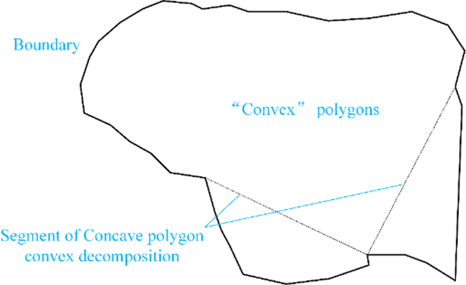
“Convex” polygons after decomposition.

The iteration process continues until no concave polygons arise. The flow chart for the concave polygon convex decomposition is shown in Figure 5.

Figure 5.

Flowchart of the concave polygon convex decomposition.

Global survey route optimizing considering optimal consumption

The previous sections finished the convex decomposition of a concave polygon. Then there exist three properties: (1) the direction of the track centerlines, (2) the track spacing, (3) the arrangement and connection of sets of track centerlines. We firstly discuss the first and third properties.

Wesley ²⁴ had demonstrated that the optimal path adopts a sweep direction perpendicular to the longest edge of the obtained convex polygon, which would minimize the cost of making turns with an AUV. We adopt Wesley’s outcome directly and this results in ladder-shaped routes regarding to those divided convex polygons, as Figure 6.

Figure 6.

The optimal global survey route for a concave polygon with a combination of track lines for separate convex polygons. (Tracking line space was set to 50 m, a fixed value considering the single seabed type).

The connection of sets of track centerlines with respect to each generated convex polygon is an optimal arrangement problem. As this example, the solution space contains $4^n\cdot {\text{A}}_{n-1}^{n-1}$ possible answers. We employs a genetic algorithm (GA) to tackle this classical traveling salesman problem. The cost function is composed of factors like energy consumption and time consumption, as following

$\text{min}\hspace{0.17em}{\text{C}}_l=k_1\cdot {\displaystyle \sum E\left(d_l,{\alpha }_l\right)}+k_2\cdot {\displaystyle \sum T\left(d_l,{\alpha }_l\right)}\hspace{0.17em}\hspace{0.17em}l\in \left\{L\right\}$

4

where $E\left(d_l,{\alpha }_l\right)$ and $T\left(d_l,{\alpha }_l\right)$ are the AUV energy and time consumption, respectively, while tracking a set of straight lines. Both E and T are functions of the track line $\hspace{0.17em}l$ . $d_l$ is the route length. ${\alpha }_l$ is the angle between the ocean current and the straight line that can also be expressed as $〈l,\hspace{0.17em}{v}_{\text{c}}〉$ . k₁ and k₂ are both positive parameters and their relationship is $k_1+k_2=1$ . The line set $\left\{L\right\}$ includes the respective track lines of convex polygons and the connecting lines of the survey route between convex polygons. Figure 6 shows the optimal global survey route after the evolving operation.

Ladder survey route optimizing method based on single convex polygon

As to the second property of the survey route, this section mainly discusses an approximate optimal optimizing method whose track spacing is able to be adjusted adaptively for the purpose of maximizing the detection performance.

Track spacing of the survey route is another property that should receive attention. It is important to the mission accomplishment quality because of the fact that underwater detection performance depends on both the sonar range and the seabed type, which is summarized by David and colleagues. ¹⁴ Therefore, a method for calculating the track spacing is developed with the objective of achieving an approximately optimal detection probability.

The sonar range and the seabed type are the two main factors affecting underwater acoustic detection. The NATO Undersea Research Centre (NURC, currently Centre for Maritime Research and Experimentation—CMRE) conducted many sea trails and reached a conclusion, shown in Figure 7(a), that can be referred to in response to this issue. ^14,25 Here, for a fixed reference distance between the AUV and the seabed set as 45.0 m, a relationship for the transverse range and detection probability is depicted in Figure 7(b).

Figure 7.

Probability of detection as a function of range and seabed type: (a) detection probability varies with seabed type and sonar range and (b) detection probability varies with seabed type and transverse distance.

The approximately optimal survey route optimizing method can be described as follows. The survey route is composed of parallel track centerlines. Once the geometric attribute was determined, the probability of detection for the mission area will be acquired according to the correspondence relationship as shown in Figure 7(b). The evolving operation is choosing a more appropriate track spacing to output a survey route that achieves an approximately optimal detection performance.

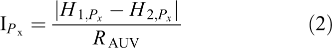
The benefit of a track is defined by the increase in the detection probability over the mission area. That is to say, it is the integration of the detection probability at each location in a track. Specifically, the benefit at location $\left(x,y\right)$ covered by a track’s swath is $B\left(x,y\right)=p\left(x,y\right)-p_0\left(x,y\right)$ , where $p\left(x,y\right)$ is the detection probability before survey, $p_0\left(x,y\right)$ is the detection probability after survey. $p_0\left(x,y\right)$ is zero in most cases indicating that we do not know the distribution of the underwater target. Let $s\left(x,y\right)$ be the seabed type at position $\left(x,y\right)$ and $d_{{\text{track}}_i}\left(x,y\right)$ be the transverse distance from the AUV. $p\left(x,y\right)$ is updated according to $p\left(x,y\right)=\text{max}\left\{p_0\left(x,y\right),p_{{\text{track}}_i}(s\left(x,y\right),\hspace{0.17em}d\left(x,y\right)),\cdots \right\}$ . Where $p_{{\text{track}}_i}(s\left(x,y\right),\hspace{0.17em}{d}_{{\text{track}}_i}\left(x,y\right))$ is the detection probability of position $\left(x,y\right)$ corresponding to sweep line track _i and the value is acquired using Figure 7(b) as a look up table. The apostrophe shows that the position $\left(x,y\right)$ is within the swath of multiple sweep lines. The seabed type $s\left(x,y\right)\in$ [sand (S), mud (M), clay (Cy), silt (Si), stone (St), rock (R), coral (Co), shells (Sh)] can be retrieved through a sea chart of the given area such as the one shown in Figure 8.

Figure 8.

Sea chart of the Yellow Sea, Weihai offshore, red rectangle is the mission region.

Here, the mission area in the Yellow Sea near Weihai is composed of flat sand and stone, as shown by the ground truth seabed map in Figure 9.

Figure 9.

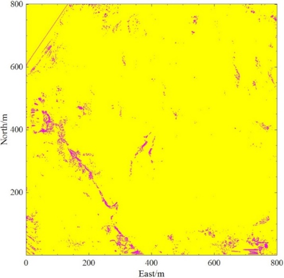
Seabed type map for the mission region, the Yellow Sea near Weihai. The yellow areas correspond to flat sand and the pink areas correspond to sand ripples.

GA is employed to act as an evolving operation. The algorithm itself inherently owns the ability to globally search for the approximately optimal result. The iteration number, time consumption, and the sum of detection probability are the termination criteria. In the experiments, a uniformly spaced track is adopted as the comparison method. For each of the two approaches considered, a set of N = 8 tracks was selected.

The locations of the actual tracks selected by the two different approaches are displayed, overlaid on the mission area’s seabed map, in Figure 10.

Figure 10.

Survey routes given by the approximately optimal track-spacing method and the uniform method. (Note that the figure is stretched horizontally to more clearly display the tracks)

Maps that qualitatively show the final detection probability everywhere in the mission area resulting from the selected set of tracks of the two approaches are shown in Figure 11. In addition to the maps in Figure 11, the performance of the two approaches is also summarized quantitatively. Figure 12 shows the proportion of the mission area that has a final probability of detection above a given value.

Figure 11.

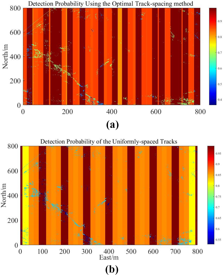
Probability of detection maps from performing a certain set of 8 tracks: (a) using the approximately optimal track-spacing method and (b) using the uniformly spaced tracks.

Figure 12.

Proportion of cells in the mission area whose probability of detection is above any value between 0 and 1 for the two cases considered.

As can be seen from the above figures, the proposed adaptive track-spacing approach clearly achieves a higher mean probability of detection than by employing uniform track spacing.

The AUVs and route following control system

In our approach, we adopt different AUVs with different control surfaces to verify the following control algorithm. Just as shown in Figure 13, AUV1 owns only one rudder just like a boat, while AUV2 has two vertically symmetrical rudders. Details of both AUVs are listed in Table 1. This kind of AUV that possesses no direct transverse and vertical control output is called an underactuated AUV. Maneuvered mostly by a single propeller and control surfaces, they are usually employed to conduct long range survey missions because of their high efficiency and reliability. Their control outputs are assumed only in three degrees, including surge, pitch, and yaw, while roll being assumed stable to simplify the analysis.

Figure 13.

With different types of control surfaces, two AUVs were used to conduct the ladder survey experiment: (a) AUV1 equipped with side-scan sonar to detect undersea objects and (b) AUV2 equipped with wide swath bathymetry system. AUV: autonomous underwater vehicle.

Table 1.

AUV parameters and configurations.

Item/unit	Value-AUV1	Value-AUV2
Overall length (mm)	1965	4400
Diameter (mm)	260	530
Mass (kg)	82.7	580 ± 5
Ultimate depth (m)	100	1000
Voyage (km)	100	300
Ultimate/cruising speed (km)	5.0/2.0	6.0/2.5
Moment of inertia Ix , Iy , Iz (kg·m2)	0.76/22.27/22.16	21.06/712.51/699.28
Actuator system	Propeller × 1, wing × 2, rudder × 1	Propeller × 1, wing × 2, rudder × 2
Motion sensor	DVL, compass, pressure sensor	DVL, compass, pressure sensor, acoustic altimeter, inertial navigation equipment
Detecting sonar	SeaKing 325 side-scan sonar	GeoSwath Plus wide swath bathymetry system

AUV: autonomous underwater vehicle; DVL: doppler velocity log.

Correspondingly, the route following control method was developed adjusting to this type of AUVs. A global survey route is decomposed and stored by sequenced points of which each connects two straight track lines (Figure 16). It can also be described as two adjacent points determining one straight track line. The route following was accomplished once the sequenced track lines have been successfully traversed. For practical application, the control law is given in discrete form.

Architecture of the route following controller

The structure of control system is a three-layered rational behavior model consisting of a task layer (strategic level), a guidance layer (tactic level), and an execution layer. The controller architecture we adopt for following a global survey route could be described by the flow chart in Figure 14.

Figure 14.

Three-layer rational behavior model-based route following controller architecture.

The guidance layer and the execution layer jointly execute the previous straight-line tracking. The task layer takes charge of the track line updating. The route following task finishes when all of the track lines composing a global survey route are traversed. As kernel content, the following sections describe how a straight-line tracking control algorithm works.

Using straight-line tracking in the horizontal plane as an example, the guidance layer calculates and gives a reference heading angle based on the relative position deviation between the AUV and the track line after the iteration begins. The application is similar to those in unmanned surface vehicle (USV) control. ²⁶ The execution layer calculates and provides instructions to the actuators to eliminate the heading angle deviation. Here, it is a rudder angle limited to a certain degree.

In this article, we discuss the controller of route following in the planar plane. Compared with a high-speed torpedo, most AUVs execute survey tasks at a relatively low speed without drastic and complex tactical actions. Therefore, it is rational to decouple the 3-D tracking into a horizontal action and vertical action individually. Considering that planar current is a very common occurrence, horizontal motion control is additionally challenging. Therefore, it is appropriate to use horizontal route following as the more representative example to be described.

The coordinate system and velocity composition law

Figure 15 shows the 3-D coordinate systems and six-degree state variables of the AUV. $\text{E}-\xi \eta \zeta$ is the inertial coordinate system. $\text{G}-xyz$ is the body-fixed coordinate system. The position and attitude vector is $\eta =\left[\xi \hspace{0.17em}\eta \hspace{0.17em}\zeta \hspace{0.17em}\varphi \hspace{0.17em}\theta \hspace{0.17em}\psi \right]$ . The velocity vector is $\nu =\left[u\hspace{0.17em}v\hspace{0.17em}w\hspace{0.17em}p\hspace{0.17em}q\hspace{0.17em}r\right]$ . Obviously, the vector $\eta$ is expressed by the component of the inertial coordinate and the vector $\nu$ is expressed by the body-fixed coordinate.

Figure 15.

Coordinate systems and AUV motion state variables. AUV: autonomous underwater vehicle.

Under the ocean current environment, the velocity of an underactuated AUV is composed of the ocean current induced velocity ${\nu }_{\text{C}}$ , and the longitudinal velocity u, which is parallel with axis $\text{G}-x$ . In Figure 16, ${\nu }_{\text{Ref}}$ is the reference velocity given by the tracking control system. It is controllable directly by the longitudinal thrust and the steering torque. The resultant velocity ${\nu }_{\text{Cmp}}$ is the element that directly eliminates the transverse deviation. The larger the transverse component of ${\nu }_{\text{Cmp}}$ , relative to the straight track line, the sooner the transverse deviation is eliminated.

Figure 16.

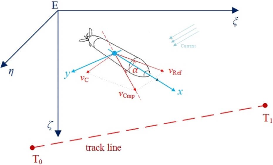
Velocity composition in straight line tracking.

The principle of implementing line tracking for an underactuated AUV can be expressed as calculating a reference heading angle and achieving it and the AUV strides forward longitudinally and moves toward the line transversely in the mean time under the velocity synthesis.

Calculation of transverse deviation

The transverse deviation is calculated according to the relative position relationship between the AUV position and the previous track line. Projected onto the horizontal plane, ${\text{S}}_{{\text{T}}_{\text{0}}{\text{-T}}_{\text{1}}}{|}_{\zeta =0}$ is the directional line from $T_0\left({\xi }_0,{\eta }_0\right)$ to $T_1\left({\xi }_1,{\eta }_1\right)$ where $T_{\text{0}}$ and $T_{\text{1}}$ are the adjacent survey route points that determine the previous track line. ${\psi }_0$ is the direction angle of the track line expressed as

${\psi }_0=\{\begin{array}{l}\text{sgn}\left({\eta }_1-{\eta }_0\right)\cdot \pi /2\hspace{0.17em}\hspace{0.17em}\hspace{0.17em}\hspace{0.17em}\hspace{0.17em}\hspace{0.17em}\hspace{0.17em}\hspace{0.17em}\hspace{0.17em}\hspace{0.17em}\hspace{0.17em}\hspace{0.17em}{\xi }_0={\xi }_1\\ \text{arctan}\left(\left({\eta }_1-{\eta }_0\right)/\left({\xi }_1-{\xi }_0\right)\right)\hspace{0.17em}\hspace{0.17em}\hspace{0.17em}\hspace{0.17em}\hspace{0.17em}\hspace{0.17em}{\xi }_1>{\xi }_0\\ \text{arctan}\left(\left({\eta }_1-{\eta }_0\right)/\left({\xi }_1-{\xi }_0\right)\right)+\pi \hspace{0.17em}\hspace{0.17em}\hspace{0.17em}\hspace{0.17em}{\xi }_1<{\xi }_0\end{array}$

5

where $P_{\text{s}}\left({\xi }_0,{\eta }_0\right)$ is the position of AUV, and $\psi \text{s}$ is the heading angle. The distance to the route is shown in the following equation

$|P_{\text{e}}|=\frac{|{\xi }_{\text{s}}\cdot ({\eta }_1-{\eta }_0)+{\eta }_{\text{s}}\cdot ({\xi }_0\text{-}{\xi }_1)+{\xi }_1\cdot {\eta }_0-{\xi }_0\cdot {\eta }_1|}{\sqrt{{({\eta }_1-{\eta }_0)}^2+{({\xi }_0\text{-}{\xi }_1)}^2}}$

6

It is defined that $P_{\text{e}}>0$ when the AUV is located on the left of vector $\stackrel{\rightharpoonup }{T_0{T}_1}$ . Meanwhile, the sign of P_e depends on the cross product of vectors $\stackrel{\rightharpoonup }{P_{\text{s}}{T}_1}$ and $\stackrel{\rightharpoonup }{T_0{T}_1}$ .

$\text{sgn}\left(P_{\text{e}}\right)=\text{sgn}\left[\left({\xi }_1-{\xi }_0\right)\cdot \left({\eta }_1-{\eta }_{\text{s}}\right)-\left({\xi }_1-{\xi }_{\text{s}}\right)\cdot \left({\eta }_1-{\eta }_0\right)\right]$

7

Combining the last two equations, P_e is calculated by the following equation

$P_{\text{e}}=\text{sgn}\left(P_{\text{e}}\right)\cdot |P_{\text{e}}|$

8

Guidance controller based on intelligent PID algorithm

The guidance controller takes P_e as the control input and calculates the compensating angle ${\psi }_{\text{c}}$ . Finally, the reference heading angle is given by the following equation

${\psi }_{\mathrm{Ref}}={\psi }_{\text{0}}+{\psi }_{\text{c}}\left(P_{\text{e}}\right)$

9

The structure of the horizontal straight line tracking control system is shown in Figure 17.

Figure 17.

Structure of horizontal straight line tracking control system.

As Figure 17 shows, the guidance controller is a single input single output (SISO) system. The controlled variable ${\psi }_{\text{c}}\in \left\{\psi |-\pi /2\le \psi \le \pi /2\right\}$ is only a function of the deviation P_e. A PID algorithm is chosen to manipulate the compensating angle ${\psi }_{\text{c}}$ . The basic PID control law can be expressed by the following equation.

$y\left(t\right)=k_{\text{p}}\cdot \epsilon \left(t\right)+k_{\text{i}}\cdot {\displaystyle {\int }_0^t\epsilon (t)\hspace{0.17em}\text{d}t+}{k}_{\text{d}}\cdot \frac{\text{d}\epsilon (t)}{\text{d}t}$

10

During the implementation of the AUV’s control system, the PID algorithm should be expressed in numerical differential form as shown in equation (11).

${\psi \prime }_{\text{c}}(n+1)=k_{\text{p}}\cdot {P\prime }_{\text{e}}(n)+k_{\text{i}}\cdot {\displaystyle \sum _{i=n-M_{\text{I}}}^n{P\prime }_{\text{e}}(i)}+k_{\text{d}}\cdot \frac{1}{M_{\text{D}}}{\displaystyle \sum _{i=n-{\text{M}}_{\text{D}}}^n{P\prime }_{\text{e}}(i)-}{P\prime }_{\text{e}}(i-1)$

11

${P\prime }_{\text{e}}(n)$ is the normalized transverse deviation employing the Sigmoid function. k _p, k _i, and k _d are the coefficients of proportion, integration, and differentiation, respectively. n is the clock for the control system. In our lab, the control period of the AUV will be set to 0.5 s if the maximum speed is lower than 3 m/s. M _I is calculating the periods of integration. M _D is a smoothing parameter usually set between 6 and 12 based on empirical evidence. A mapping relationship between the PID output ${{\psi }^{\prime }}_{\text{c}}$ and the compensating heading angle ${\psi }_{\text{c}}$ is constructed based on the Sigmoid function.

${\psi }_{\text{c}}=\frac{\pi }{2}\cdot \left(\frac{2.0}{1.0+e^{-3{{\psi }^{\prime }}_{\text{c}}}}-1.0\right)$

12

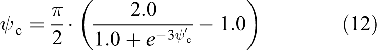
The mapping relationship curve is shown in Figure 18.

Figure 18.

Basic Sigmoid curve.

The guidance controller is enlightened by the Lyapunov theory. Our goal is to eliminate ${\text{P}}_{\text{e}}\to 0$ . The Lyapunov function is shown in equation (13).

$V=\frac{1}{2}{P}_e^2$

13

Obviously, the only balanced state for the tracking system occurs at the origin point $P_{\text{e}}=0$ . The scalar function $V$ is a positive definite if $P_{\text{e}}\ne 0$ . If $P_{\text{e}}\to 0$ , then $V\to \infty$ correspondingly. As P_e is a real measurement of the AUV’s relative space position, its value changes continuously. The physical meaning of the derivative ${\dot{P}}_{\text{e}}$ is the velocity of the AUV approaching the track line in the planar plane. The function V has a continuous derivative expressed in equation (14).

$\dot{V}\text{=}{\dot{P}}_{\text{e}}\cdot P_{\text{e}}$

14

If P_e and ${\dot{P}}_{\text{e}}$ are opposite signs throughout the process, this means that $\dot{V}\hspace{0.17em}\text{< 0}$ . We can then draw a conclusion that the guidance controller is large-scale asymptotic convergent. Obviously, the guidance design thought is to raise the opposite sign ${\dot{P}}_{\text{e}}$ against P_e. An underactuated AUV is only able to adjust its vector direction of velocity through the course angle.

Therefore, the relationship between ${\dot{P}}_{\text{e}}$ against P_e is converted to a function from P_e to ${{\psi }^{\prime }}_{\text{c}}$ . ${\dot{P}}_{\text{e}}$ is certain to change while ${\psi }_{\text{c}}$ varies. Under the circumstance of $P_{\text{e}}>0$ , the PID controller generates a heading angle toward the track line. If an ocean current exists, the integral section accumulates and a larger ${\psi \prime }_{\text{c}}$ is given so that ${\dot{P}}_{\text{e}}$ continually acts until P_e is back to zero.

A fuzzy mechanism is introduced to improve the control quality. Generally speaking, to increase the speed of the system response, a relatively larger k _p is needed when the transverse deviation is large. To make the system more stable, a larger k _d is needed when the transverse deviation is small. k _i should also be adjusted as the AUV approaches. The variable P_e and ${\dot{P}}_{\text{e}}$ are described as fuzzy sets. The adaptive PID control parameter adjustment proceeds as shown in formula (15)

$\left[k_p,k_i,k_d\right]=Fuzzy\left({\dot{P}}_{\text{e}}\text{,}\hspace{0.17em}{P}_{\text{e}}\right)$

15

The following provides details about the fuzzy adaptive adjustment of the control parameters. The fuzzy subsets are expressed as $P_{\text{e}}=\left\{\cdots ,\text{Z,S,M,L,E}\right\}$ , ${\dot{P}}_{\text{e}}=\left\{\cdots ,\text{Z,S,M,L}\right\}$ , and $\left[k_p,k_i,k_d\right]=\left\{\cdots ,\text{Z,S,M,L}\right\}$ . The symbol $\cdots$ represents the negative subset elements. The membership functions are shown in Figure 19. As a result of symmetry, only the conditions of $P_{\text{e}}>0$ are listed. The fuzzy rules are set as shown in Tables 2 to 4.

Figure 19.

Membership functions of fuzzy subsets.

Table 2.

Fuzzy rules of k _p.

P e k p ${\dot{P}}_e$	NE	NL	NM	NS	Z	S	M	L	E
NL	L	L	L	L	Z	NM	NS	S	M
NM	L	L	L	L	Z	NS	S	M	L
NS	L	L	L	M	Z	Z	S	M	L
Z	L	L	M	M	Z	M	M	L	L
S	L	M	S	Z	Z	M	L	L	L
M	L	M	S	NS	Z	L	L	L	L
L	M	S	NS	NM	Z	L	L	L	L

Table 3.

Fuzzy rules of k _d.

P e k p ${\dot{P}}_e$	NE	NL	NM	NS	Z	S	M	L	E
NL	L	L	L	L	L	M	S	Z	Z
NM	L	L	L	L	M	S	Z	Z	NS
NS	L	L	L	M	S	Z	Z	NS	NM
Z	Z	Z	Z	Z	Z	Z	Z	Z	Z
S	NM	NS	Z	Z	S	M	L	L	L
M	NS	Z	Z	S	M	L	L	L	L
L	Z	Z	S	M	L	L	L	L	L

Table 4.

Fuzzy rules of k _i.

P e	NE	NL	NM	NS	Z	S	M	L	E
k i	Z	Z	S	M	Z	M	S	Z	Z

Execution controller designed on S-surface function

In horizontal line tracking, the execution controller eliminates error between the AUV heading angle and the reference angle given by the guidance controller. As the reference angle varies with time, the control performance such as rapidity and stability seem much more important. The improved S-surface control algorithm ²⁷ is adopted, as in equation (16)

$N^{\prime }=\frac{2}{1+\text{exp}(k_{\text{1}}{\psi \prime }_e+k_{\text{2}}{\dot{{\psi }^{\prime }}}_e)}-1+\Delta N_0$

16

${\psi \prime }_{\text{e}}$ and ${\dot{{\psi }^{\prime }}}_{\text{e}}$ are the normalized heading angle error and its deviation. N′ is the normalized steering torque. $\Delta N_0$ is normalized static disturbance adjusting torque that usually comes from the system state offset. It should be set permanently and the value will be acquired through step response of heading control trails in still water pool. k₁ and k₂ are the adaptively adjusting control parameters composed of a constant term and an adjusted term as

$k_{1,2}=k_{\text{c}}+k_{\text{a}}$

17

in which k _a is defined by equation (18)

$k_{\text{a}}=C_1\text{sgn}\left({\dot{{\psi }^{\prime }}}_{\text{e}}\cdot {\psi \prime }_{\text{e}}\right)+C_2|{\psi \prime }_{\text{e}}|+C_3|{\dot{{\psi }^{\prime }}}_{\text{e}}|$

18

where C ₁, C ₂, and C ₃ are the weight parameters.

Similar to the PD algorithm, the output of the S-surface algorithm varies with the deviation and its derivative, as Figure 20. The nonlinear feature gives it better performance. The parameter adaptive operation also helps to improve the performance.

Figure 20.

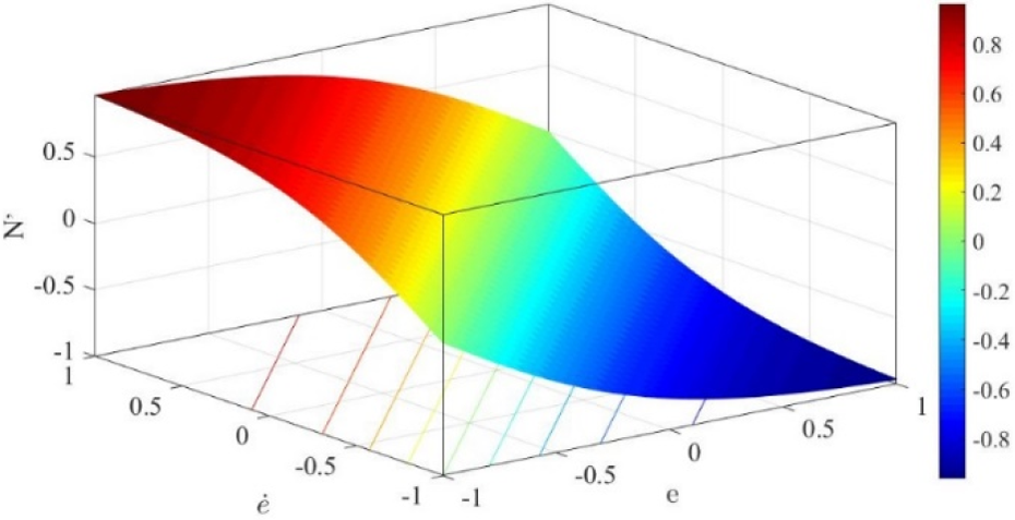
The input and output relationship of S-surface function.

Figure 21 shows part of the route following test result at the Chinese Yellow Sea in 2015. Together with Figure 22, the heading angle was able to follow both the time-varying reference angle and the step change reference angle under the steering of heading controller. The accuracy and stability of the controller are expressed by the step signal following test.

Figure 21.

Time-varying reference heading angle tracking result during the route following experiment at sea.

Figure 22.

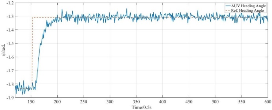
Step response of heading angle tracking control experiment at sea.

Experimental verification

Experimental details

A series of coverage survey experiments were conducted to verify the route following control method. Experiments were carried out successively in the Longfeng Lake located in the Southern Heilongjiang province and at the Yellow Sea adjacent to Weihai, Shandong province. The route following test data of the lake trials and sea trials were obtained under the same control parameters. Details of the two experiments are provided in Table 5.

Table 5.

Experimental conditions.

Item	Value
	Lake	Sea
Region size (m2)	2000 × 400	600 × 600
Main directional length (m)	2000	600
Route interval (m)	110	100
Cruising speed (m/s)	1.00	1.20
Sailing depth (m)	2.00	3.00
Time consumption (min)	139.7	42.5

Ladder survey results

Lake experiment

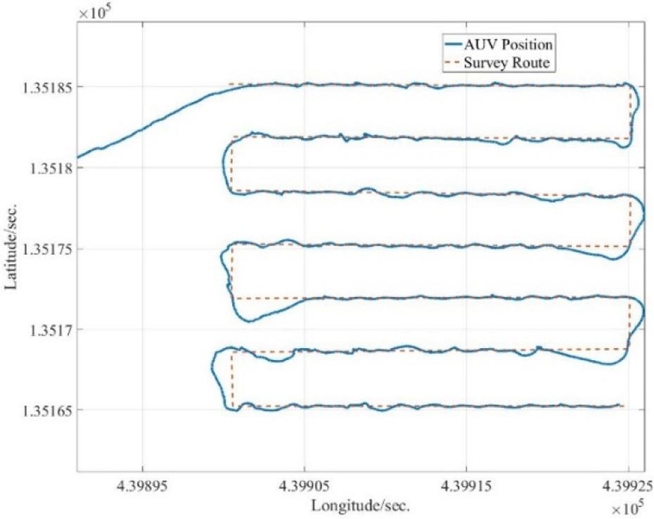
We performed the survey test using AUV1 in Longfeng Lake. The sailing is composed of an underwater survey and surfacing navigation correction. Operations at a 3-m depth underwater and surface sailing were alternately carried out. The switch acts according to time and position. The AUV sails underwater first for 600 s then rises up to the surface with global positioning system (GPS) correction for 30 s. After finishing line tracking in the main direction, the AUV must float upward to correct its position. The current in the lake is relatively small and steady. Figures 26 and 27 show the route following results. The equipped SeaKing SSS works to detect underwater objects. The detection range was set to 30 m. Figures 23 to 25 show the acquired sonar images after recovery.

Figure 23.

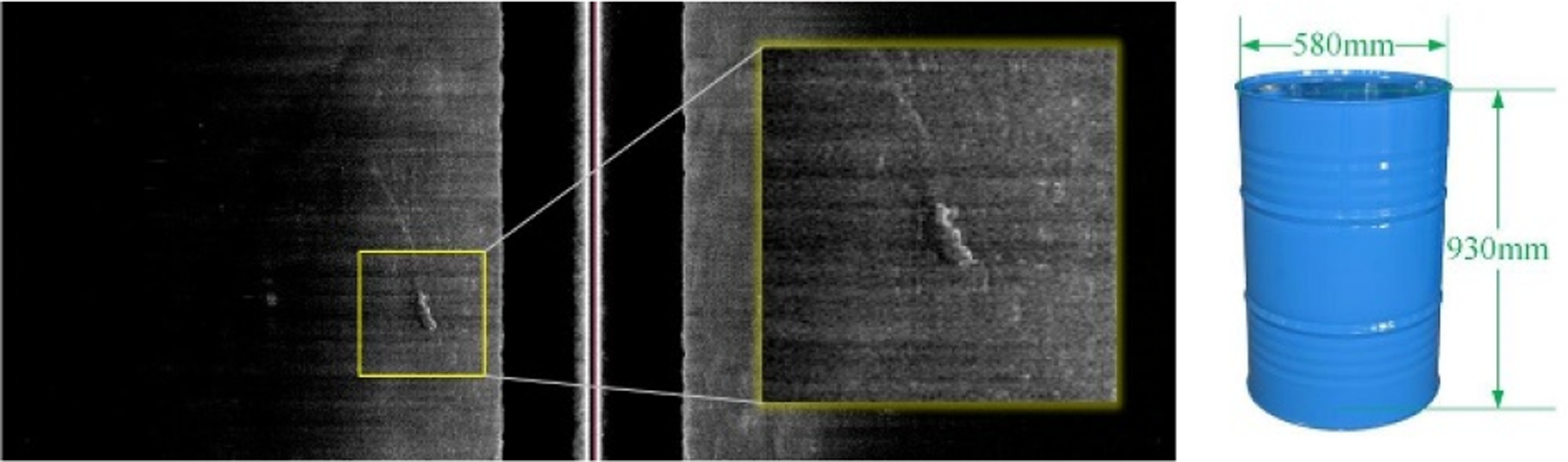
Submerged object detection result using side-scan sonar for a prepositioned oil drum.

Figure 24.

Side-scan sonar image of a sunken fishing boat in Longfeng lake.

Figure 25.

Side-scan sonar image of terrain features.

Figure 26.

Latitude and longitude contrast between the AUV track and the target route. AUV: autonomous underwater vehicle.

Figure 27.

Tracking error curve of lake test.

Figure 26 shows the case of a comb-shaped route following. The corresponding error curve is shown in Figure 27. Off-route motion occurred with a maximum error of 32 m. This is because of navigation correction while the AUV floats upward and GPS information arrives. From Figure 27, we can determine that even though diving and surfacing movements occurred, the tracking accuracy of the main part was less than 1.0 m.

Sea experiment

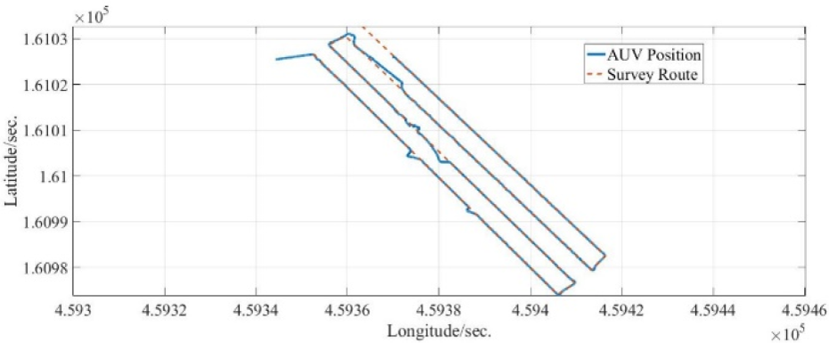
The currents composed of the tide current and the Yellow Sea costal wind current was very complex in the testing area. AUV2 carried out an ongoing underwater self-sailing lasting 40 min. AUV2 tracked a comb-shaped route and sailed at a permanent depth of 3 m. The ladder survey route and AUV trail are compared in Figure 29. Figure 30 shows the tracking error. The error jumps to a larger value while the track line switches. The equipped GeoSwath Plus sonar worked throughout the AUV cruising course. The terrain map was drawn as shown in Figure 28 by us according to the detection data after recovery. The swath width was set to 90 m.

Figure 28.

Ocean floor relief map acquired by AUV2 equipped with a GS+ underwater terrain mapping instrument. The color bar indicates the depth. AUV: autonomous underwater vehicle.

Figure 29.

Latitude and longitude contrast between AUV track and target route. AUV: autonomous underwater vehicle.

Figure 30.

Tracking error curve of sea test.

As shown in Figure 29, the tracking result is compared to the comb path expressed as a red line. From Figure 30, we determine that the AUV was able to track the global path well but that the tracking error was large and reached 30.40 m while updating the target route. There are many reasons for this which involve the rough description of the path without considering the AUV maneuverability and the disturbance of the current. After that, the tracking error converged within the normal range of 0–2.0 m from a larger value of 15–30 m gradually in the process of tracking a longer route.

Conclusions

In this article, a complete control structure involving AUV autonomous coverage detection missions including survey route optimizing and following control is proposed.

Firstly, an off-line global survey route with a ladder shape is planned combining the given mission restrictions and an electronic sea chart. The route is composed of parts according to the mission region decomposition conditions because of the invisibility of the concave polygon. This means that even faced with a geometrically concave harbor, our method will still be able to output a coverage survey route. Furthermore, instead of uniformed track lines, the track spacing of the ladder survey route is optimized according to the detection performance of the sonar aimed at maximizing the detection probability. Simulation experiments show that the proposed track-spacing optimization method clearly achieves a higher mean probability of detection under the same consumption condition.

Secondly, the route following controller is designed. We adopt a decoupled and three-layered structure that does not rely on a mathematical model of the AUV. The lower two layers are mainly described and tested. The guidance layer computes the reference angle of yaw or trim according to the position deviation in the horizontal plane or the vertical plane. A PID algorithm is adopted with its parameters adaptively adjusted according to the varying position deviation and deviation rate. The guidance controller plays a key role in resisting the interference of ocean currents. The execution layer computes execution instructions such as rudder angle or wing angle to generate the maneuvering force aimed at attitude angle. The experiment at sea shows that the adaptive nonlinear S-surface function acts rapidly and steadily during the process of following a varying reference heading angle.

The proposed controller with parallel parameters was applied in different AUVs to conduct different coverage detection missions under different circumstances. The ladder survey results demonstrate the robustness of our controller. Sailing in rough sea conditions demonstrates that the controller is accurate and steady when facing time varying environmental disturbances.

Future work will refer to the study of applying the whole technical system to various coverage missions such as underwater terrain mapping in the fields of marine geography, biology, or vehicle navigation, submerged objects detection in the maritime or military fields, and even sunken dead body discovery in the field of criminal justice. Another key problem concerns the smooth motion restriction considering the underwater detection performance brought by sonars. This seems somewhat contrary to the rapidity and precision of the route following controller. Therefore, a balance between the performance of the controller and the detection performance should be taken into consideration.