Using synthetic basis feature descriptor for motion estimation

Abstract

Development of advanced driver assistance systems has become an important focus for automotive industry in recent years. Within this field, many computer vision–related functions require motion estimation. This article discusses the implementation of a newly developed SYnthetic BAsis (SYBA) feature descriptor for matching feature points to generate a sparse motion field for analysis. Two motion estimation examples using this sparse motion field are presented. One uses motion classification for monitoring vehicle motion to detect abrupt movement and to provide a rough estimate of the depth of the scene in front of the vehicle. The other one detects moving objects for vehicle surrounding monitoring to detect vehicles with movements that could potentially cause collisions. This algorithm detects vehicles that are speeding up from behind, slowing down in the front, changing lane, or passing. Four videos are used to evaluate these algorithms. Experimental results verify SYnthetic BAsis’ performance and the feasibility of using the resulting sparse motion field in embedded vision sensors for motion-based driver assistance systems.

Introduction

Motion estimation is an important step to solving computer vision problems such as visual odometry, ¹ depth from motion, ² structure from motion, ³ navigation, and many others. These are common problems in applications like video surveillance, ⁴ robot navigation, ⁵ and advanced driver assistance systems (ADAS). ⁶ ADAS are designed to include safety features to avoid accidents by altering the driver of potential problems or even taking over the control of the vehicle to ensure or improve driving safety. These features may include automatic lighting control, adaptive cruise control, automatic braking, traffic warnings, and so on. They may also alert the driver of approaching vehicles and unintended lane departure.

A vehicle may be driven in urban, suburban, or rural environments and with a variety of road conditions, speeds, daylight conditions, and seasons. Driving situation is quite unpredictable for ADAS applications especially when other moving vehicles and pedestrians are involved. ⁷ Motion estimation accuracy in different driving situations is critical to the performance of ADAS.

Many vision-based algorithms for ADAS applications are reported in the literature. Only a few are included as representations of this exciting field. De la Escalera et al. proposed an algorithm to detect and recognize traffic signs, ⁸ which includes the knowledge used while designing the signs and is immune to lighting changes and occlusion. A survey on traffic sign detection was reported in the study by Møgelmose et al. ⁹

Another important function for ADAS is lane detection and lane departure warning. A video-based lane estimation and tracking system using steerable filters was developed for robust and accurate lane-marking detection. ¹⁰ Pixels belong to the lane markings are filtered and fit to a lane model that is coherent with the perspective of the scene for a lane departure warning system. ¹¹

Road detection and tracking is critical to autonomous driving. Stereovision-based algorithms were reported to reliably detect both planar and nonplanar road surface. ^12,13 Road boundary and nearby vehicle detection algorithm was developed to estimate their relationships with the host driving lane for expanding the usability of lane-keeping assist, adaptive cruise control, and precrash safety for urban driving conditions. ¹⁴

Pedestrian detection recognition ^15,16 and driving assistance in dense fog ¹⁷ are added features to assist and increase driving safety. Collision warning or anti-collision systems have been widely used and perhaps the most driving safety feature. A few examples include an automatic braking system based on driver’s pedal deflection timing, ¹⁸ a collision warning system that adjusts the warning threshold according to the driver behavior changes, ¹⁹ and obstacle detection and localization. ²⁰

Motion estimation methods can be grouped into two categories. One uses feature matching techniques to find corresponding features between two image frames to obtain a sparse motion field. The other one uses differential techniques based on spatial and temporal variations of the image brightness to obtain a dense motion field. There is usually large camera or object movement or long baseline between frames for ADAS applications. Differential techniques may not be suitable for ADAS because they work well mostly for very small movement (short baseline).

In this research, we implement our newly developed SYnthetic BAsis (SYBA) feature descriptor ²¹ for matching feature points to generate a sparse motion field for analysis. SYBA is a simple and hardware-friendly feature descriptor that does not require square root, division, or exponential operations that require floating-point computations. It reduces the computational power requirement, increases the speed and accuracy of feature matching, and to use it for real-time embedded vision applications. It has been successfully used for reconstructing the global view of the soccer field from broadcast soccer game video for play annotation, ²² camera pose estimation, ²³ and for unmanned air vehicle target tracking. ²⁴ Its most recent application was for visual odometry drift reduction for autonomous vehicles. ²⁵

In this article, we adapt the SYBA descriptor to motion field generation and developing two motion estimation algorithms for potential ADAS applications. The first function is a motion classification algorithm for camera motion estimation to detect abrupt movements of the vehicle and to provide a rough estimate of the depth of the scene in front of the vehicle. Based on two frames, the camera motion is classified into four different situations: (1) pan left, (2) pan right, (3) sensor receding, and (4) sensor approaching. This algorithm is also able to roughly estimate the depth of the scene in front of the vehicle to suggest a safe path. Experiments are performed on two videos captured from a camera onboard a moving vehicle to demonstrate its effectiveness.

The second function is a vehicle surrounding monitoring algorithm to detect movement of the surrounding vehicles that could potentially cause threat or collision. Input image frames are processed one by one to match feature points between two frames to obtain a homography. This homography matrix is used to transform and align the previous frame to the current frame to detect the movements of surrounding vehicles. A warning signal can be generated when vehicles are speeding up from behind, slowing down in the front, changing lane, or passing. Two videos are used to evaluate the performance of this vehicle surrounding monitoring algorithm.

The remainder of this article is organized as follows. Details of SYBA descriptor are presented in the second section. The third section introduces the motion classification algorithm and the fourth section discusses the vehicle surrounding monitoring algorithm. The fifth section evaluates the performance of our algorithms with videos of a variety of real-world outdoor environments. The final section concludes and summarizes our findings.

SYBA descriptor

Inspired by the recent development of a new compressed sensing theory, ²⁶ our new SYBA feature descriptor is developed to find the best matching feature pairs between two image frames. Compared with other efficient feature descriptors, ^21,25 SYBA is a robust feature description and matching algorithm that performs well with the presence of illumination, blurring, rotation, and perspective variations. It is a hardware-friendly algorithm and requires only a minimal amount of memory space, which makes it a perfect choice for feature description in real-time robotic vision applications and hardware implementation for embedded vision sensor applications.

SYBA descriptor provides a unique description of the surrounding region of a feature point so that features from two images but with similar descriptor elements can be matched accurately. To form a unique descriptor with the SYBA algorithm, the input image frame is processed with the procedure shown in the flow diagram in Figure 1. SYBA has been proven to be better or comparable to other widely used feature descriptors. Thorough comparisons between SYBA and SIFT, SURF, BASIS, D-BRIEF, TreeBASIS, BASIS384, and BRIEF-32 are presented in our previous work. ²¹ A summary of the SYBA algorithm is presented in the following subsections.

Figure 1.

Flowchart of the SYBA descriptor algorithm. SYBA: SYnthetic Basis.

Feature detection

Feature detection is performed on the input image frame to locate feature points whose surrounding region will be described by SYBA. Generally, many feature detection algorithms could be employed here. In this work, SURF is selected to detect feature points for its performance and popularity as well as the convenience and fairness for comparisons. ²¹ For most real-time vision applications, a simple but robust feature detector such as Harris corner detector ²⁷ would be more suitable for hardware implementation and still provide adequate performance.

Binary feature region image

For each detected feature point, a small surrounding region is cropped and saved as its feature region image (FRI). To include sufficient information to uniquely represent the FRI and decrease the risk of containing too much nonessential information, a 30 × 30 FRI is used for each feature point. Reducing the size may risk losing information that is needed to uniquely represent the feature region. ²¹

The average intensity of the 900 pixels in the 30 × 30 FRI is used as a threshold to binarize the FRI. Pixels brighter than the threshold are set to 1 and set to 0 otherwise. Figure 1 shows an example of the binary FRI (BFRI) of a selected feature point. The BFRI provides a rough quantization to the surrounding region of detected feature points, while includes the spatial and structural information of the feature region. It also provides a certain degree of illumination invariance.

Compressed sensing theory

The basic idea of the compressed sensing theory is to use random patterns to describe a signal. ²⁶ Using this theory, a small image region can be described by a series of randomly generated synthetic basis images (SBIs) to construct a descriptor for feature matching. SBIs are sparse images with a binary value at each pixel location. We use normally distributed pseudo-random numbers to generate these SBIs. They are only generated once and can be reused. The number of SBIs required is directly related to the size of the image region to be described ²⁶

$M=C\left(K\text{ln}\frac{N}{K}\right)$

1

where N is the number of pixels of an SBI which has the same size as the image region to be described and K is the number of pixels in the SBIs with a value ‘1’. M is the number of SBIs required to describe the image region. The value M is minimum when $K=N/2$ . The value M increases as K differs from $\frac{N}{2}$ .

We divide the 30 × 30 BFRI of a feature point into thirty-six 5 × 5 nonoverlapping subregions and generate 5 × 5 SBIs to describe each of these subregions. The number of pixels in a subregion of BFRI, N, is 25. According to equation (1), the minimum number of SBIs, M, is $13\times \hspace{0.17em}\text{ln}\left(25/13\right)=9$ if the number of pixels with a value ‘1’ in each SBI is 13 ( $K=N/2$ ). Every SBI is generated with normally distributed pseudo-random numbers. Experimentally, using a subregion larger than 5 × 5 does not improve the feature matching accuracy enough to justify its increased computational costs. The comparisons of performance with different sizes of BFRI are reported in the study by Desai et al. ²¹

Feature description

Every subregion with a size of 5 × 5 is described by measuring the similarity between the subregion and the nine SBIs. As all subregions of the BFRI and the nine SBIs have binary values, the similarity is measured by counting how many pixels with a value ‘1’ in a 5 × 5 subregion of the BFRI also have a value ‘1’ at the correspondence position in the SBIs. The SYBA similarity measure (SSM) can be expressed as equation (2)

${\text{SSM}}_i={\displaystyle {\sum }_{\left(x,y\right)}\left[{\text{BFRI}}_s\left(x,y\right)\cdot {\text{SBI}}_i\left(x,y\right)\right]}$

2

where ${\text{BFRI}}_s\left(x,y\right)$ is a subregion of the BFRI, and ${\text{SBI}}_i\left(x,y\right)$ is one of the randomly generated patterns with the same size as the ${\text{BFRI}}_s\left(x,y\right)$ . The summation is performed within the subregion, which is 5 × 5 in this work.

Figure 2 shows how the similarity is measured. Figure 2(a) shows nine randomly generated 5 × 5 SBIs. Figure 2(b) shows a 30 × 30 BFRI that is divided into 6 × 6 nonoverlapping 5 × 5 subregions. Pixels with a value ‘1’ are marked in WHITE, while the pixels with a value ‘0’ are marked in BLACK. Figure 2(c) shows the SSM between the upper left subregion of the BFRI and SBI #1. The SSM is 2 because 2 corresponding pixels have a value ‘1’ in both the subregion and the SBI #1. Similarly, as shown in Figure 2(d), the SSM between the same upper left subregion of the BFRI and SBI #2 is 10.

Figure 2.

(a) Nine 5 × 5 synthetic basis images labeled 1 to 9, (b) a 30 × 30 BFRI that is divided into thirty-six 5 × 5 subregions, (c) similarity measure between the highlighted 5 × 5 subregion and the first SBI, and (d) similarity measure between the highlighted 5 × 5 subregion and the second SBI. BFRI: binary feature region image; SBI: synthetic basis image.

The maximum SSM is 13 since there are only thirteen 1s in an SBI (K = 13). An SSM ranging from 0 to 13 requires 4 bits for storage. This similarity measure method yields nine SSMs for each subregion. The nine SSMs are stacked into a vector to describe a subregion. Concatenating vectors for all 36 subregions forms a SYBA descriptor for an FRI. A SYBA descriptor requires 1296 bits (36 subregions × 9 SSMs × 4 bits) to describe an FRI.

Feature matching

Feature points can be matched by comparing their SYBA descriptors. We use the L1 norm rather than other common comparison metrics such as Euclidean or Mahalanobis distance, which require complex operations such as multiplication and square root, to minimize the computational complexity.

Figure 3 shows an example of comparing two feature descriptors. Descriptor-1 and Descriptor-2 are SYBA descriptors for two feature points. The difference between each SSM from these two descriptors are recorded in the bottom row. The summation of all SSM differences is regarded as the difference between these two feature points. A difference value close to zero indicates an excellent match. A large value represents a poor match.

Figure 3.

The SYBA descriptor comparison for feature matching. SYBA: SYnthetic Basis.

To find the best matching feature, each feature in the first image is compared against features in the second image. Of the L1 values computed against the features in the second image, the minimum is found to determine the best matching feature. For the pair to be uniquely matched, the computed best match for the corresponding feature in the second image must also be the best match to the original feature in the first image. Otherwise, no match is chosen for the feature. Features are also ranked based on the difference in L1 norm values between the best match and the second-best match in the second image. To obtain fewer matched pairs but higher matched precision, thresholds can be used to reject matched pairs with a small difference in L1 norm matching distances between the first and second-best matches. ²¹

Motion classification and depth estimation

Motion field is the result of pixel movement from image to image caused by moving camera or moving objects in a 3-D scene. Each vector in the motion field represents the motion of a feature point in the image. A motion field can be formed as a result of the vehicle’s movement such as turn, forward, and reverse. Four simple and ideal motion fields representing common driving scenarios are shown in Figure 4. When a vehicle makes a right turn, all feature points move from right to left in successive frames as shown in Figure 4(a). The opposite of this motion is when the vehicle makes a left turn and all feature points move from left to right as shown in Figure 4(b). Similarly, as shown in Figure 4(c), as the vehicle approaches the scene, all feature points diverge from the focal point (or vanishing point). They all converge to the focal point when the vehicle pulls away from the scene.

Figure 4.

Ideal motion fields. (a) Right turn, (b) left turn, (c) approaching, and (d) receding.

Motion field

In this study, instead of analyzing and tracking individual feature points, we attempt to detect the moving vehicles and analyzing their motion as a whole. To achieve this goal, a sparse motion field must be generated. The motion field is constructed with a number of motion vectors between two successive frames. Motion vectors between two frames are established by matching corresponding features using SYBA as described in “Feature matching” section. Motion vectors are represented in polar coordinates (magnitude and orientation) for vehicle motion classification. Depth estimate is performed by segmenting the motion field into different regions based on the length of motion vectors.

The motion vector magnitude is the distance between the two matching points. The motion orientation is the angle between the vector connecting the two matching points and the vertical axis pointing up. A motion vector aligned with the vertical axis is assigned an orientation of 0° and the positive angle increases in the clockwise direction and negative angle increases in the counterclockwise direction.

Figure 5(a) shows a typical motion field that represents the orientation of motion vectors in degrees. Figure 5(b) is the zoomed in detail of the highlighted red rectangular region shown in Figure 5(a). The green crosses in Figure 5(a) indicate the feature point locations in the first frame and the red circles indicate the matching features in the second frame. The yellow line connecting a green cross to its corresponding red circle represents the length of the motion vector. Figure 5(c) shows how motion vector orientation is defined. Positive angle increases in clockwise direction. Whereas, negative angle increases in counterclockwise direction. In the example in Figure 5, most motion vectors shown in Figure 5(a) are around −90° according to our definition. This motion field represents a right turn motion, which has most of the motion vectors pointing to the left and approximately −90° from the vertical axis counterclockwise.

Figure 5.

(a) An example of sparse motion field, red circles represent the end points of the motion vectors; (b) zoomed in motion field in the red rectangle to highlight the orientation details; and (c) definition of motion vector orientation.

Motion classification

Our motion classification algorithm is based on a simple statistical analysis of motion vector orientation distribution. This simple classification algorithm is able to classify vehicle motion into four simple motions as shown in Figure 4. Using the motion field shown in Figure 6(a) as an example from a video captured in Provo, Utah. This motion field is generated by matching features between two consecutive frames. In this example, the vehicle makes a right turn at an intersection and the motion field is very similar to the one shown in Figure 4(a). The majority of the motion vectors point to the left in roughly −90° as defined in “Feature matching” section.

Figure 6.

Experiments on a video captured in Provo, Utah. (a) Feature points from the previous frame (green crosses) are matched to feature points in the current frame (red circles). (b) Motion vectors near the camera have the largest movement (red regions). The furthest regions (least movement) are highlighted in blue. (c) and (d) Both left and right histograms peak at around −90° indicating a right turn motion.

We divide the motion field in Figure 6(a) into left and right halves. A one-dimensional histogram of the motion vector orientation distribution is constructed for each half. The histogram of the left half of the motion field is shown in Figure 6(c) and the histogram for the right half of the motion field is shown in Figure 6(d). Using a right turn motion as an example, the majority of motion vector orientations shown in Figure 6(a) in both left and right halves are close to −90° as most motion vectors pointing to the left (similar to Figure 4(a)). Figure 6(c) and (d) shows that the left and right histograms both peak at around −90° which indicates a right turn motion.

Table 1 summarizes motion vector distributions for the left and right histograms for each motion. For example, for a right turn motion (Figure 4(a)), the majority of motion vectors are close to −90°, which results in both left and right histograms peaking at close to −90°. For a left turn motion (Figure 4(b), most motion vectors point to the right, which results in both left and right histograms peaking at close to 90°.

Table 1.

Motion vector distribution for motion classification.

Motion class	Right turn	Left turn	Approaching	Receding
Motion field	Figure 4(a)	Figure 4(b)	Figure 4(c)	Figure 4(d)
Left histogram	Peak at −90°	Peak at 90°	Peak at −90°	Peak at 90°
Right histogram	Peak at −90°	Peak at 90°	Peak at 90°	Peak at −90°

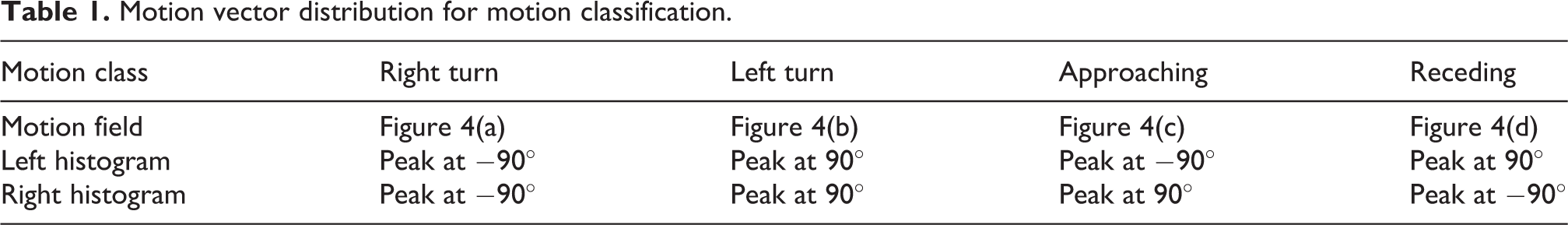
When the vehicle approaches the scene (Figure 4(c)), the majority of motion vectors move away from the focal point, which results in the left histogram peaking at around −90° and the right histogram peaking at around 90°. On the contrary, when the vehicle pulls away from the scene (Figure 4(d)), the majority of motion vectors converge to the focal point, which results in the left histogram peaking at around 90° and the right histogram peaking at around −90°. By examining the peak point in the histograms for the left and right halves of the motion field, the vehicle motion can be classified into one of the four motions shown in Figure 4.

Depth estimation

Depth estimation is performed by segmenting the motion field into different regions based on the length of motion vectors. Feature points that are close to the camera move more or faster between frames than those that are farther away from the camera. A series of thresholds in number of pixels on the length of motion vectors are selected to segment the motion field (Figure 6(a)). Figure 6(b) shows the motion vector length segmentation result. Motion vectors near the camera having the large movement are segmented and shown in red. The farthest regions (least movement or shortest motion vectors) or regions without many motion vectors (road region and regions without feature points) are highlighted in blue. This simple depth estimation method provides a rough estimate of the 3-D scene and can be used to estimate the time to impact or for obstacle detection. This rough estimate of distance is by no means a replacement of other more reliable 3-D sensing devices such as stereovision sensor or LIDAR. It simply provides a rough estimate of the vehicle’s surroundings to the autonomous vehicle system and to assist the system to adjust its control on the vehicle.

Vehicle surrounding monitoring

Vehicle surrounding monitoring is critical to the detection of potential collisions. In this research, we focus on detecting vehicles that are speeding up from behind, slowing down in the front, changing lane, or attempting to pass. All these scenarios require motion estimation.

Homography

Homography is a transformation matrix used often in computer vision. It relates any image of the same planar surface in space to another. Many features can be used to calculate the homography matrix, like lines and conics. Using feature correspondence of small patches is the most common and straightforward method.

Depth variations of feature points affect the homography accuracy. We assume and use the weak-perspective camera model for this application. The weak-perspective camera model assumes that the average distance of feature points is much larger than the distance variations within the scene (or among feature points). There are always errors in the homography matrix caused by depth variations. The motion vectors constructed from images include both inliers and outliers. Outliers are the points that have inconsistent movement from the majorities. Ideal motion fields such as those shown in Figure 4 are not realistic. Real motion fields always include outlier motion vectors. We apply the RAndom SAmple Consensus (RANSAC) technique to detect and exclude outliers from homography calculation.

Vehicle detection

Our vehicle detection algorithm makes three assumptions that we believe are reasonable: (1) Majority of the motion vectors in a motion field are the result of the relative motion between the background and camera. (2) Vehicles of interest (speeding up from behind, slowing down in the front, changing lane, or attempting to pass) have motions distinct from the background. (3) Vehicles that maintain the same motion as the camera or with very small relative motion with the camera move the same or almost the same as the background and can be treated as the background.

We use the inlier motion vectors from matching SYBA descriptors to compute a homography matrix to transform and align two consecutive frames to calculate their absolute difference. Vehicles with motions different from the background can be detected by thresholding the absolute difference image. Vehicle movement or intention can be estimated by its location in the image from frame to frame. This is a simple but effective approach for detecting moving objects or objects with noticeable relative motion with the camera.

Experimental results

Motion classification and depth analysis

Our motion classification and depth analysis methods were tested using one new video captured in Provo, Utah and one from the KITTI data set. ²⁸ All videos were captured in different traffic scenarios and at different locations. As a result, these videos have different light conditions, shadow presence, and different numbers of cars, pedestrians, cyclists, bikers, and high slopes.

Figure 7 shows results from the video captured in Provo, Utah that includes a left turn motion, an approaching and receding sensor. This video also includes a right turn motion that is used as an example in Figure 6. For the left turn motion (Figure 7(a)), both left and right histograms peak at approximately 90° (all motion vectors pointing to the right) as defined in Table 1. For the sensor approaching motion (Figure 7(b)), the majority of motion vectors in the left half of the motion field have a negative motion vector orientation (pointing to the left). The majority of motion vectors in the right half of the motion field have a positive motion vector orientation (pointing to the right). This motion field indicates a motion of approaching as shown in Figure 4(c).

Figure 7.

Motion classification and depth analysis results of (a) left turn, (b) camera approaching, and (c) camera receding motions.

For the sensor receding motion (Figure 7(c)), the motion field is the opposite to the previous case. The majority of motion vectors in the left half of the motion field have a positive motion vector orientation (pointing to the right). The majority of motion vectors in the right half of the motion field have a negative motion vector orientation (pointing to the left) indicating a motion of receding as shown in Figure 4(d). All histograms have some negligible noise from motion vectors pointing in other directions. Most of them are in vertical directions and are from feature points in the sky and feature points in the road regions in front of the vehicle.

Depth estimation was performed by segmenting these motion fields in to regions for different depths. Segmentation was performed based on the length of motion vectors. Feature points in the regions that are close to the camera or vehicles have long motion vectors. Whereas, those in the regions that are farther from the camera have very short motion vectors. The distances are color coded in Figure 7. Regions such as the sky and the road that do not have sufficient motion vectors are coded with dark blue. These depth maps show regions that are safe and can be used to calculate the time to impact or provide a rough estimate of depth.

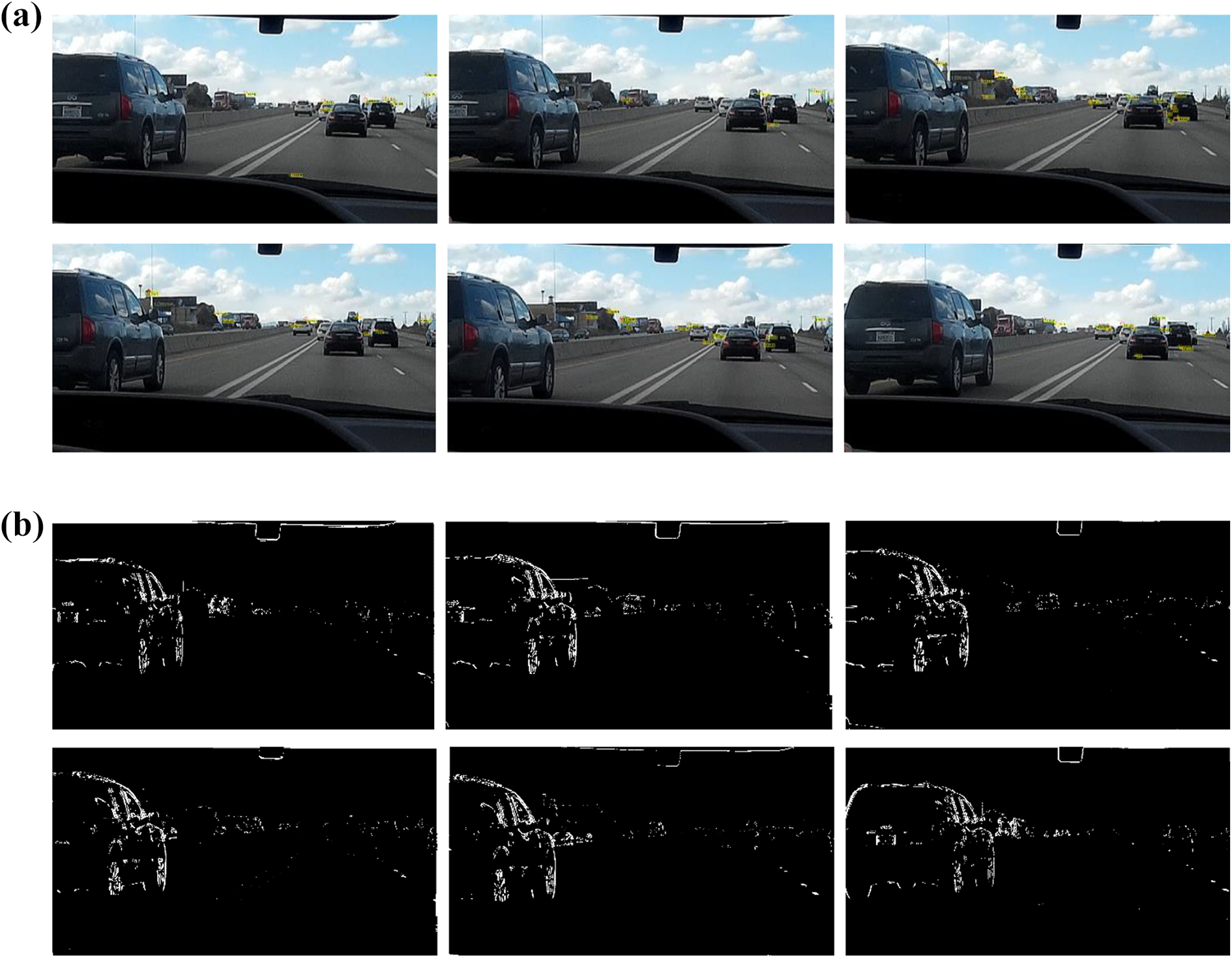
One KITTI sequence was tested in the same manner. Example feature matching results using the SYBA descriptor are shown in the left column in Figure 8. As shown in the figures, feature points from the previous frame (green crosses) are matched to feature points in the current frame (red circles). The motion direction is classified based on the statistical analysis of motion vector orientation presented in “Motion classification” section. The right turn motion has both histograms peak at around −90°. Whereas, the forward motion has the left histogram peak at −90° and the right histogram peak at 90°. Depth estimation results are shown in the upper right corner. This video involes illumination and viewpoint changes to demonstrate the performace of our algorithm.

Figure 8.

Experiment on the KITTI data set (a) Right turn, (b) camera approaching, and (c) left turn.

Vehicle surrounding monitoring

We recorded two videos for vehicle surrounding monitoring experiments. The first was collected with a stationary camera. In this case, the background in the video was still and only the vehicle had a relative motion. We used this video to test and confirm our first two assumptions discussed in “Vehicle detection” section. The second video was recorded with the camera mounted on a vehicle moving on a highway. We used this video to confirm our third assumption.

Figure 9 shows results from the first video. Figure 9(a) shows six sample frames from the video with the detected inlier motion vectors. The green crosses indicate the locations of feature points in the previous frame, and the red circles indicate the locations of corresponding feature points in the current frame. Since only the inliers are shown in the figure and the camera is stationary, all inlier matching features have no motion in the image and motion vectors are with zero length. Figure 9(b) shows details of a few motion vectors in a small zoomed in area. The results of the absolute difference are shown in Figure 9(c). The location of vehicle in the image indicates its movement from left to right.

Figure 9.

Results from video with a stationary camera. (a) Sample frames with motion vectors, (b) cropped and zoomed in area to show details of a few motion vectors, and (c) detected vehicle.

Since there is no relative motion between the camera and the background, ideally, after removing the outliers mainly from the moving vehicle, the calculated homography should have no transformation effect. In other words, if SYBA performs well and feature matching is accurate, the resulting absolute difference obtained from the transformed images should be exactly the same or very close to the absolute difference from images without transformation. Figure 9(c) shows result of perfect feature matching.

We noticed that there were not many motion vectors or not many matched feature points in Figure 9(a). They were sufficient to compute an accurate homography. Fewer good matching feature points are arguably better than more but low-quality matching feature points.

Figure 10 shows results from the second video. In this case, the camera moved forward toward the background. There were also other vehicles moving at about the same speed as the camera. On the left of the images, there was a vehicle passing our vehicle so its speed was slightly higher. As shown in Figure 10(a), the two vehicles in front of the camera and with very small relative motion to the camera were treated as the background and their motion vectors were treated as inliers for homography computation. The motion vectors caused by the passing vehicle were treated as outliers and were not included for homography computation. As shown in Figure 10(b), only the passing vehicle and vehicles moving in the opposite direction were detected.

Figure 10.

Results from video with a moving camera. (a) Sample frames with motion vectors and (b) detected vehicle.

Conclusion

In this article, we have presented our new SYBA feature descriptor for accurate feature matching and have introduced two motion analysis algorithms. Motion vectors are calculated in polar coordinates for statistical analysis to classify the vehicle motion and estimate the depth information of the 3-D scene in front of the vehicle. Depth analysis is performed by segmenting the motion field into different regions based on the length of motion vectors. Depth information can be used for time-to-impact calculation or obstacle detection. The vehicle surrounding monitoring algorithm detects vehicles that could potentially cause collision. Both algorithms are simple but efficient.

Our qualitative analyses confirmed the effectiveness and robustness of our algorithms for videos captured in different environments. The experimental results also show that the SYBA descriptor worked very well with a variety of image deformations such as illumination, blurring, shadows, and camera movement caused by pan and tilt. ²¹ Comparing to other methods, SYBA descriptor requires a smaller descriptor size, lower computational complexity, less computation time, and less memory requirements to match feature points. ²¹ It is an excellent candidate for hardware implementation for real-time vision applications. Our algorithms using the SYBA descriptor are computationally inexpensive and can be easily integrated into most ADAS applications that rely on accurate feature matching.

Our next step is to implement this algorithm in hardware such as field programmable gate arrays to explore the possibility of building an embedded vision sensor for the proposed motion analysis algorithms and other ADAS applications. More experiments need to be done to further evaluate their performance for more complicated situations.