A single acoustic beacon-based positioning method for underwater mobile recovery of an AUV

Abstract

This article presents a navigation method for an autonomous underwater vehicle being recovered by a human-occupied vehicle. The autonomous underwater vehicle is considered to carry underwater navigation sensors such as ultra-short baseline, Doppler velocity log, and inertial navigation system. Using these sensors’ information, a navigation module combining the ultra-short baseline positioning and inertial positioning is established. In this study, there is assumed to be no communication between the autonomous underwater vehicle and human-occupied vehicle; thus, to obtain the autonomous underwater vehicle position in the inertial coordinate, a conjecture method to obtain the human-occupied vehicle coordinates is proposed. To reduce the error accumulation of autonomous underwater vehicle navigation, a method called one-step dead reckoning positioning is proposed, and the one-step dead reckoning positioning is treated as a correction to combine with ultra-short baseline positioning by a data fusion algorithm. One-step dead reckoning positioning is a positioning method based on the previous time-step coordinates of the autonomous underwater vehicle.

Introduction

Currently, autonomous underwater vehicles (AUVs) are used to perform many ocean missions. Typically, AUVs perform missions that can last between 16 h and 24 h. Human-occupied vehicles (HOVs) have the ability to operate for a long time in standby in the open ocean and have a large capacity for carrying several AUVs; however, they are not suitable for long-range ocean exploration operations. In contrast, AUVs are suited for scouting in littoral seas. AUVs can perform some tasks that surface ships and HOVs cannot carry out conveniently and safely. The RAND company recommended the following seven mission categories for AUVs in a report in 2009 ¹ : mine countermeasures, missions to deploy leave-behind surveillance sensors or sensor arrays, near-land and harbor monitoring missions, oceanography missions, monitoring of undersea infrastructure, anti-submarine warfare tracking missions, and inspection/identification missions. A large-scale HOV equipped with AUV can carry out scientific inspection operations in a wider range and with higher efficiency, and it is of great significance for the detection of unknown hazards. An HOV can improve its overall capability by carrying AUVs; this has become a trend in HOV mission modes.

Rendezvous and docking between an AUV and HOV is the key technology for HOVs carrying AUVs. Many methods to recover AUVs and dock them with an HOV have been proposed, such as Watt et al.’s proposed method of an active dock robotic manipulator system (a quasi-independent third body). ^2,3 Hardy and Barlow proposed a dry deck shelter recovery method. ⁴ Moody designed a recovery device in the torpedo tube of the submarine. ⁵ General Dynamics Electric Boat designed an SSGN Universal Launch and Recovery Module in the launch tube. ⁶ Kimball et al. demonstrated the applicability of autonomous docking in robotic exploration of sub-ice oceans; the vehicle can approach the dock from any direction. ⁷ Piskura et al. designed a line capture line recovery system, one of the key technologies in digital ultra-short baseline (DUSBL) navigation and homing. ⁸ Plueddemann et al. used the USBL navigation system during the recovery of an AUV in sea ice. ⁹

The navigation and location of an AUV is an important factor in the rendezvous and docking process, especially under the limiting conditions of underwater observation. Therefore, it is meaningful to consider accurate navigation methods during the rendezvous and docking process.

The different methods that are currently used for AUV navigation during the recovery process can be grouped into three categories:

Inertial navigation: Inertial navigation uses gyroscopic sensors to detect the acceleration of the AUV, and it can be combined to obtain the Doppler velocity log to obtain a more accurate measurement. Combining this information with the attitude information measured by compass is an integral operation to obtain the vehicle’s track. ^10,11 A problem with inertial navigation is that the navigation errors are accumulated.

Acoustic navigation: Acoustic navigation uses acoustic transponder beacons to allow the AUV to determine its position. Acoustic navigation systems are generally classified by the length of the baseline, that is, the distance between the active sensing transponders. The most common acoustic navigation systems for AUV navigation are long baseline, which uses at least two widely separated transponders, and USBL. ¹⁰ Taking USBL positioning as an example, the AUV is equipped with a transducer that transmits a pulse interrogation signal to a transponder deployed in the HOV. The transponder, after receiving the interrogation pulse signal, transmits a reply pulse signal different from the interrogation signal. The calculation of the position within the system is based on the distance and azimuth of the transponder and the coordinates of the AUV relative to the position of the HOV in three dimensions. Batista et al. installed USBL on the nose of the AUV, and a sensor-based integrated guidance and control is proposed using the USBL positioning system. ¹²

Visual navigation: Visual navigation is divided into two methods. One is feature detection and image analysis, which exhibits high accuracy and successful detection of the sought points. However, the camera is also sensitive to many factors (turbidity, level of light), and the target should be in a line-of-sight condition. The other method is photocell light sensing, which also has a high accuracy but only in limited directions. The system is less complicated than feature detection and image analysis but also sensitive to similar factors. ^13,14

However, each navigation method has its own inherent limitations, and so a single sensor may not be sufficient to provide a suitable navigation system. Therefore, it is preferable to use a number of sensors and combine their information to provide the necessary navigational capability. To achieve this, a multi-sensor data fusion (MSDF) approach can be used. MSDF is an information processing technology that has been rapidly developed in recent years. It integrates multi-sensor or multi-source information and data, resulting in more accurate and reliable conclusions. Khan et al. fused the USBL data with a particle filter estimate of dead reckoning, and the simulation and field experiments verify the performance of MSDF. ¹⁵

In general, MSDF provides significant benefits over single source data. The application of this technology can improve both the accuracy and robustness of the AUV navigation system and shorten the system response time. In data fusion, the weighted fusion algorithm is a mature fusion algorithm. Its optimality, unbiasedness, and minimum mean-square error have been proved in many research results. The problem with the weighted fusion algorithm is how to determine the weight, and the choice of weight directly affects the fusion result.

The article is organized as follows: The second section introduces the process of AUV recovery and navigation positioning. A method for conjecturing the velocity and heading of an HOV is presented in the third section. The fourth section presents a detailed description of the design of the navigation filter. The fifth section presents inertial navigation positioning based on the position of the previous moment fused with the USBL positioning data. The last part introduces the simulation experiment.

The process of docking and location

Generally, in order to simplify a docking mission, it is assumed that the HOV is traveling in a race track at a low velocity during the rendezvous process, which consists of two long straight track legs and two semicircle track legs as shown in Figure 1. Recovery can be thought of as taking place in three stages ¹⁶ :

Initial stage. When the AUV reaches around the recovery area (at position A), it broadcasts the acoustic signals by the transducer. While the HOV receives the signal, it will travel along a fixed heading, and the execution stage is started.

Execution stage. The AUV is moving from position A to A′. During this stage, the AUV captures the HOV position and uses the navigation data to control itself, thus reducing the distance between AUV and HOV by adjusting the proper position, speed, and attitude conditions for the recovery stage.

Recovery stage. The AUV is moving from position A′ to B′. During this stage, the recovery operation is complete. This part is not in the scope of the research content of this letter.

Figure 1.

Three stages of AUV underwater mobile recovery. AUV: autonomous underwater vehicle.

This study investigated the positioning method of stage 2, which is outside the range of vision location. Therefore, the positioning method should be selected between acoustic positioning and inertial positioning.

The principle of positioning is to measure the position of something relative to a certain point. In other words, we need to know at least two coordinates. With static repositioning as an example, generally, in the stationary docking process, the AUV locates itself through the USBL positioning system. The AUV position can be calculated by

$P_{\text{auv}}\left(t\right)=P_{\text{dev}}\left(t\right)-\Delta L\left(t\right)$

1

where $P_{\text{auv}}\left(t\right)$ is the position of the AUV, $P_{\text{dev}}\left(t\right)$ is the position of the docking device, and $\Delta L\left(t\right)$ is the USBL measurement value.

The coordinates of the docking station are fixed values and are usually set as the origin of the coordinate system. The relative distance between the docking station and the AUV can be obtained through the USBL ranging system, so that the positioning of the AUV can be realized. However, in the process of an HOV recovering an AUV, it is not sufficient to measure the relative distance of them. The navigation system should acquire the position of the HOV to realize the positioning of the AUV. That means

$P_{\text{auv}}\left(t\right)=P_{\text{hov}}\left(t\right)-\Delta L\left(t\right)$

2

In other words, the recovery process requires the AUV to obtain the coordinates of the AUV and the HOV at the same time. Underwater communication is not conducive to HOV concealment, and frequent underwater communication will increase the chance of HOV exposure. Therefore, this study was based on an assumption that during the recovery process, there is no communication between the HOV and AUV.

Equation (2) places the requirements of the position of the HOV; a new method is proposed to replace the underwater communication to obtain the HOV positions. As shown in Figure 1, during the docking process, the HOV undergoes uniform linear motion at a fixed depth. If the AUV knows the velocity and the heading of the HOV, the coordinate of the HOV could be obtained at any time step.

The process of obtaining the velocity and heading of an HOV is called a conjecture process; the details are described in the following sections.

The flowchart in Figure 2 illustrates the location process:

The AUV arrives at the grounding point at the appointed time and receives a signal from the HOV’s single beacon (dock connection) to establish a temporary coordinate system.

The conjecture process is started and the speed and heading of the HOV are calculated on the basis of the single beacon signal. After the calculated speed and heading are stable, the conjecture process is completed.

The origin of the coordinate system is translated to the current AUV position (updated AUV coordinates) and the current position of the HOV is measured via USBL.

One-step dead reckoning (OSDR) positioning is combined with the UBSL positioning method.

After every 25 s, the speed and heading of the HOV are updated.

Figure 2.

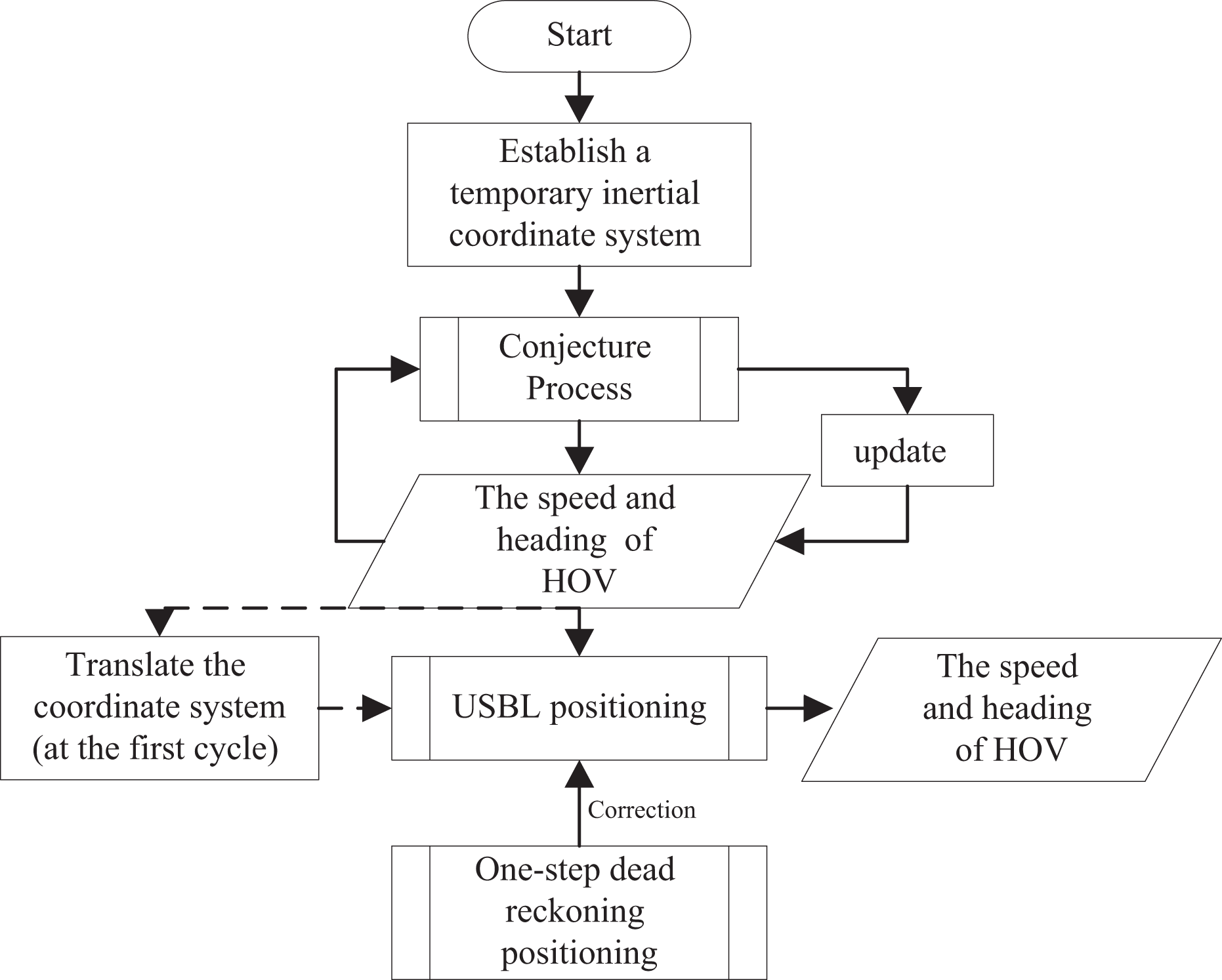
Flowchart of the location method process.

The conjecture process, USBL positioning, and OSDR correction are explained in detail in the following sections.

The conjecture process

The conjecture process is started at the same time as the execution stage. The AUV is equipped with a transducer that transmits a pulse interrogation signal to a transponder deployed in the HOV. The transponder, after receiving the interrogation pulse signal, transmits a reply pulse signal different from the interrogation signal. The coordinates of the AUV relative to the HOV are calculated at each cycle.

In the first conjecture process, an inertial coordinate $E-\xi \eta \zeta$ is established. For convenience, the origin of the coordinate system is set to the initial position of the AUV. To reflect the generality of the study, the $\xi \eta$ -axes are set randomly and the ζ-axis is perpendicular to the horizontal plane.

Under the coordinate system $E-\xi \eta \zeta$ , the AUV can obtain its coordinates by the dead reckoning system. At the same time, the relative position of the AUV and HOV can be measured with USBL, and according to equation (2), the position coordinates of the HOV can be calculated. The error of the USBL positioning is approximately 0.5–1.5% of its slant distance and the distance between AUV and HOV is around 1000–2000 m. At the start of recovery process, the error of the USBL positioning is around 10–20 m and the speed of HOV is around 3–5 kn. To accurately measure the HOV’s speed and heading, the measurement distance of HOV is empirically set to 100 m during the conjecture process and the measurement time is set as 50 s. After the measurement is completed, the time series $T\left(n\right)$ and the HOV position sequence $P_{\text{hov}}\left(n\right)$ are obtained.

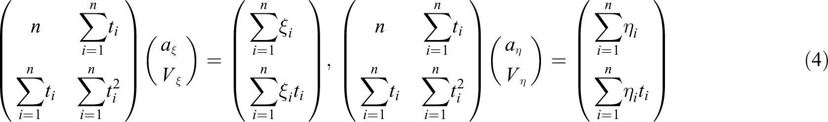
Then, the heading of the HOV can be calculated by ¹⁷

$\begin{array}{l}\left(\begin{array}{cc}n& {\displaystyle \sum _{i=1}^n{\xi }_i}\\ {\displaystyle \sum _{i=1}^n{\xi }_i}& {\displaystyle \sum _{i=1}^n{\xi }_i^2}\end{array}\right)\left(\begin{array}{l}a\\ b\end{array}\right)=\left(\begin{array}{l}{\displaystyle \sum _{i=1}^n{\eta }_i}\\ {\displaystyle \sum _{i=1}^n{\eta }_i{\xi }_i}\end{array}\right)\\ \psi =\text{tan}\left(\frac{a}{b}\right)\end{array}$

3

where η_i and ξ_i are the coordinates of the HOV at t_i and ψ is the heading of the HOV.

Then, the velocity of the HOV $[V_{\xi },V_{\eta }]$ can be calculated by

$\left(\begin{array}{cc}n& {\displaystyle \sum _{i=1}^n{t}_i}\\ {\displaystyle \sum _{i=1}^n{t}_i}& {\displaystyle \sum _{i=1}^n{t}_i^2}\end{array}\right)\left(\begin{array}{l}{a}_{\xi }\\ V_{\xi }\end{array}\right)=\left(\begin{array}{l}{\displaystyle \sum _{i=1}^n{\xi }_i}\\ {\displaystyle \sum _{i=1}^n{\xi }_i{t}_i}\end{array}\right),\left(\begin{array}{cc}n& {\displaystyle \sum _{i=1}^n{t}_i}\\ {\displaystyle \sum _{i=1}^n{t}_i}& {\displaystyle \sum _{i=1}^n{t}_i^2}\end{array}\right)\left(\begin{array}{l}{a}_{\eta }\\ V_{\eta }\end{array}\right)=\left(\begin{array}{l}{\displaystyle \sum _{i=1}^n{\eta }_i}\\ {\displaystyle \sum _{i=1}^n{\eta }_i{t}_i}\end{array}\right)$

4

Navigation filter

The location system implemented in this study was a combination of two independent Kalman filters (KFs) and a data fusion module, as shown in Figure 3. The USBL KF (referred to by the letter a) is responsible for estimating the position of the AUV $\left(P_{\text{auv}}=\left[{\xi }_a,{\eta }_a,{\zeta }_a\right]\right)$ . Another KF (referred to by the letter b) is responsible for estimating the variation of AUV position $\left(\Delta P_{\text{auv}}=\left[\Delta {\xi }_a,\Delta {\eta }_a,\Delta {\zeta }_a\right]\right)$ . Then fuse the variation of AUV position that KF-a estimated as a correction with the AUV position that KF-b estimated.

Figure 3.

Proposed scheme of sensor fusion and sensor information.

After obtaining the AUV position by the UBSL positioning system, the obtained data should be filtered. In this study, considering the motion model of the AUV and HOV during recovery, a KF based on a simplified motion model is proposed. ¹⁸

As shown in the preceding discussion, in the recovery process, the HOV is constrained in a plane and moves in a straight line. In one pulse repetition period of the USBL positioning system, the AUV is considered to be at a constant speed. From the preceding conventions and assumptions, the relative motion between the AUV and HOV can be simplified to

$\Delta L_{a|k}=-\frac{1}{2}{\dot{V}}_{\text{auv}}{t}^2+\left(V_{\text{hov}}-V_{\text{auv}}\right)t+\Delta L_{a|k-1}$

5

where $\Delta L_{a|k}$ and $\Delta L_{a|k-1}$ are the measured distances of USBL for k and k−1, respectively, ${\dot{V}}_{\text{auv}}$ is the AUV acceleration, and $V_{\text{sub}}$ and $V_{\text{auv}}$ are the velocity vectors of the HOV and AUV, respectively.

The state vector is taken as

$x^a={\left[\xi ,\eta ,\zeta ,\dot{\xi },\dot{\eta },\dot{\zeta }\right]}^{\text{T}}$

6

The corresponding covariance matrix is denoted as P_a.

The sensor input $z_k^a$ is given by

$z_k^a={\left[{\xi }_k,{\eta }_k,{\zeta }_k\right]}^{\text{T}},R^a=\text{ diag}\left({\sigma }_{\xi }^2,{\sigma }_{\eta }^2,{\sigma }_{\zeta }^2\right)$

7

From the state at time k − 1, the KF uses a vehicle model to predict the states at time k

$\begin{array}{l}{\widehat{x}}_{k|k-1}^a=A^a{x}_{k-1|k-1}^a+B^a{U}_{k-1}^a\\ P_{k|k-1}^a=A^a{P}_{k-1|k-1}^a{A}^{aT}+Q^a\end{array}$

8

where the state transition matrix $A^a$ describes the vessel motion and propagates the states through time. The matrix $U_k^a$ is the control vector $U_k^a={\left[{\dot{\xi }}_k,{\dot{\eta }}_k,{\dot{\zeta }}_k\right]}^{\text{T}}$ and $B^a$ is the control-input matrix. The matrix $Q^a$ represents the process noise and is tuned according to the expected acceleration kinematics of the vehicle.

$A^a=\left(\begin{array}{cccccc}1& 0& 0& \Delta t& 0& 0\\ 0& 1& 0& 0& \Delta t& 0\\ 0& 0& 1& 0& 0& \Delta t\\ 0& 0& 0& 1& 0& 0\\ 0& 0& 0& 0& 1& 0\\ 0& 0& 0& 0& 0& 1\end{array}\right),B^a=\left[\begin{array}{cc}{0}_{3\times 3}& \frac{1}{2}\Delta t^2\cdot I_{3\times 3}\end{array}\right],Q^a=\text{ diag}\left({\sigma }_{n\xi }^2,{\sigma }_{n\eta }^2,{\sigma }_{n\zeta }^2,{\sigma }_{n\dot{\xi }}^2,{\sigma }_{n\dot{\eta }}^2,{\sigma }_{n\dot{\zeta }}^2\right)$

9

The time update of the equation of state is

$\begin{array}{l}{\widehat{x}}_{k|k-1}^a=A^a{x}_{k-1|k-1}^a+B^a{U}_{k-1}^a\\ P_{k|k-1}^a=A^a{P}_{k-1|k-1}^a{A}^{aT}+Q^a\end{array}$

10

Comparing the noise provided by the sensor $R^a$ with the a priori estimated covariance obtains the Kalman gain

$K_k^a=P_{k|k-1}^a{H}^{aT}{\left(H^a{P}_{k|k-1}^a{H}^{aT}+R^a\right)}^{-1}$

11

where $H^a$ is the measurement matrix. The estimation is updated on the basis of the Kalman gain and the sensor reading

$\begin{array}{l}{x}_{k|k}^a=x_{k|k-1}^a+K_k^a\left(z_k^a-H^a{\widehat{x}}_{k|k-1}^a\right)\\ P_{k|k}^a=\left(I-K_k^a{H}^a\right)P_{k|k-1}^a\end{array}$

12

By processing the data of the compasses, gyro, and other sensors, and then converting the coordinates, the KF-b receives the position variation of the AUV, and it performs data processing to obtain a more accurate position variation.

The second KF has the same structure as that described previously, but with the superscript a replaced with b. The state vector is taken as

$x^b={\left[\Delta \xi ,\Delta \eta ,\Delta \zeta ,\dot{\xi },\dot{\eta },\dot{\zeta }\right]}^{\text{T}}$

13

The corresponding covariance matrix is denoted as P_b and $\left[\Delta \xi ,\Delta \eta ,\Delta \zeta \right]$ is the variation of AUV position in a period.

The sensor input $z_k^b$ is given by

$z_k^b={\left[\Delta {\xi }_k,\Delta {\eta }_k,\Delta {\zeta }_k\right]}^{\text{T}},R^b=\text{ diag}\left({\sigma }_{\Delta \xi }^2,{\sigma }_{\Delta \eta }^2,{\sigma }_{\Delta \zeta }^2\right)$

14

OSDR correction

The OSDR correction improves the positioning accuracy by introducing the inertial correction data into USBL positioning. As shown in Figure 4, it is a data fusion process between USBL data and inertial correction data. However, the inertial correction data are not equal to those of the inertial navigation system. The OSDR is based on the fusion data, which is the AUV position at t − 1

$P_{\text{auv}}^{\text{osdr}}\left(t\right)=P_{\text{auv}}\left(t-1\right)+\Delta P_{\text{auv}}\left(t\right)$

15

where $P_{\text{auv}}^{\text{osdr}}\left(t\right)$ is the OSDR position at time t and $\Delta P_{\text{auv}}\left(t\right)$ is the AUV position variation.

Figure 4.

Schematic diagram of OSDR. OSDR: one-step dead reckoning.

$P_{\text{auv}}^{\text{osdr}}\left(t\right)$ and $P_{\text{auv}}^{\text{usbl}}\left(t\right)$ are both location data, so it is convenient to use the weighted average method for data fusion. The weighted average method is a simple and intuitive fusion method for real-time processing of information, and it has a good fusion effect. The general processing method of the weighted average method is as follows ¹⁹ :

At time k, the AUV uses l sets of different sensors to measure independently and obtain l sets of measurement vectors

$Z_1\left(k\right),Z_2\left(k\right),\mathrm{...},Z_l\left(k\right)$

16

The measurement of variance matrix is

$S_1\left(k\right),S_2\left(k\right),\mathrm{...},S_l\left(k\right)$

17

Then,

$\begin{array}{l}Z\left(k\right)=S\left(k\right)\left[S_1^{-1}\left(k\right)Z_1\left(k\right)+S_2^{-1}\left(k\right)Z_2\left(k\right)+\cdots +S_l^{-1}\left(k\right)Z_l\left(k\right)\right]\\ S^{-1}\left(k\right)=S_1^{-1}\left(k\right)+S_2^{-1}\left(k\right)+\cdots +S_l^{-1}\left(k\right)\end{array}$

18

where $Z\left(k\right)$ is the fusion of the measurement vector, $S\left(k\right)$ is the fusion of the variance matrix, $Z_l\left(k\right)$ is the measurement of sensor l, and $S_l^{-1}\left(k\right)$ is the variance matrix of the measurement l.

Before applying this method, the system and sensor should be analyzed in detail to obtain the correct weights. From equation (18), it is shown that weight and variance have a corresponding relationship in data fusion. However, the variance of dead reckoning is not a fixed value; according to the variance of the choice of different weights, a suitable variance model was established in this study.

The error of the USBL positioning is approximately 0.5–1.5% of its slant distance, and the dead reckoning error is approximately 0.7–1.3% of the vehicle voyage. ²⁰ Thus, the error of the OSDR positioning is related to the dead reckoning error and the error of the previous fused data. Therefore, the variance model is shown as follows

$\begin{array}{l}{S}_U\left(k\right)={\left[{\sigma }_U\cdot \Delta L\left(k\right)\right]}^2\\ S_{\text{OSDR}}\left(k\right)=S_{\text{OSDRC}}\left(k-1\right)+{\left[{\sigma }_d\cdot \Delta l\left(k\right)\right]}^2\\ S_{\text{OSDRC}}{\left(k\right)}^{-1}=S_{\text{OSDR}}{\left(k\right)}^{-1}+S_U{\left(k\right)}^{-1}\end{array}$

19

where $S_U$ is the variance matrix of USBL positioning, $S_{\text{OSDR}}$ is the variance matrix of dead reckoning, ${\sigma }_U$ is the error coefficient of USBL, $S_{\text{OSDRC}}$ is the variance matrix of data fusion, and σ_d is the error coefficient of reckoning. The $S_{\text{OSDRC}}$ and σ_d are assumed to be independent of each other.

According to the variance model $S_U$ and $S_{\text{OSDR}}$ , the variable weight of the data fusion can be calculated. According to the fusion equations (18) and (19), the USBL positioning data and the OSDR positioning data are processed to obtain the fusion data.

Simulations

This study carried out simulation verification through MATLAB and hardware-in-the-loop (HIL) simulation platform. Figure 5 shows the hardware architecture of the AUV HIL simulation platform. The planning-control computer, the USBL acoustic information processor computer, and the dead reckoning computer are the PC104 bus embedded multi-board system. The monitoring computer and dynamics simulation computer are PCs, which use Windows operating system, and receive and record the state information of AUV through network protocol and serial port protocol. Using microsoft foundation classes (MFC) as the development environment for the AUV recovery simulation system, the program of VEGA is embedded in the MFC document application framework. The visual simulation of HIL simulation is shown in Figure 6.

Figure 5.

Architecture of the AUV hardware-in-the-loop simulation platform. AUV: autonomous underwater vehicle.

Figure 6.

The interface of visual simulation.

In the MATLAB and HIL simulation, the algorithms and AUV model are same. The difference is that the time-step size of the MATLAB simulation is 0.5 s, and considering the computing power of embedded computer, the time-step size of the HIL simulation is set as 2 s. And the recovery path in simulation is shown in Figure 7. The coordinate system $E-\xi \eta \zeta$ is established at the start of communication stage. The initial position of the AUV is set at the coordinate origin. The HOV’s heading is a straight line of the in-plane motion parallel to the y-axis starting at [−230, −500, −110], and the trajectory of the AUV is divided into two parts, the first part is a quarter circle in $\xi \eta$ -plane and the second part is a curve in $\xi \zeta$ -plane. In the recovery process, the USBL time delay is less than 2 s at the start of the recovery process, and at the end, the time delay is less than 0.2 s. Because of the AUV’s smooth motion, the USBL time delay in the simulation was not considered. The simulation contained three different positioning methods: OSDR correction, USBL, and inertial navigation combined with USBL. The data processing result of MATLAB is shown in Figure 8.

Figure 7.

AUV motion trajectory diagram. AUV: autonomous underwater vehicle.

Figure 8.

AUV trajectory under different filtering methods: (a) AUV trajectory at axis ξ, (b) AUV trajectory at axis η, and (c) AUV trajectory at axis ζ. The blue line illustrates the true AUV position, the red line shows the KF of USBL positioning, the yellow line is the OSDR correction position, and the purple dotted line shows the data fusion of USBL and traditional inertial positioning. AUV: autonomous underwater vehicle; KF: Kalman filter; USBL: ultra-short baseline; OSDR: one-step dead reckoning.

The error of the OSDR correction method and that of USBL positioning and inertial positioning in MATLAB and HIL simulation are shown in Figure 9. The mean errors of each method in MATLAB and HIL simulation are shown in Table 1.

Figure 9.

Error of different filtering methods: (a) the MATLAB simulation results and (b) the HIL simulation results. The blue line is the OSDR correction positioning error, the red line shows the error of the data fusion of USBL and traditional inertial positioning, the yellow line illustrates the KF of USBL positioning, and the purple dotted line shows the measurement error. KF: Kalman filter; USBL: ultra-short baseline; OSDR: one-step dead reckoning; HIL: hardware-in-the-loop.

Table 1.

Mean error and the percentage of different filter methods in MATLAB and HIL.

Method	Mean error (MATLAB)	$\frac{\text{Error}}{e_{\text{Nosie}}}$ (MATLAB)	Mean error (HIL)	$\frac{\text{Error}}{e_{\text{Nosie}}}$ (HIL)
$e_{\text{OSDRC}}$	2.9983	0.3135	2.9711	0.3115
$e_{\text{USBL}}$	4.1658	0.4356	4.3063	0.4515
$e_{\text{Inerital}}$	3.7151	0.3884	4.0477	0.4244
$e_{\text{Nosie}}$	9.5643	1	9.5368	1

HIL: hardware-in-the-loop.

Conclusions and future research

In this article, we propose a method to conjecture the position of an HOV without communication between the AUV and HOV. The OSDR inertial positioning method is considered as a correction of the USBL position method, and their combination algorithm shows better navigation effects. The simulation showed that the accuracy of OSDR correction is better than using USBL positioning alone, and the mean error of OSDR correction is approximately 70.48% of the USBL positioning error. It is also better than the fusion of traditional inertial dead reckoning data with USBL positioning data. The error is approximately 77.05% of that of the fusion inertial positioning.

In future research, we aim to investigate some more complex scenarios involving time delay and a temporary loss of acoustic signal. Future work will also set a more realistic underwater acoustic noise model and compare the filter architecture suggested in this article with other architectures based on the extended kalman filter and particle filter.