Sage Journals: Discover world-class research

Abstract

Bevel tip flexible needle is a novel application in minimally invasive surgery, for it can avoid obstacles by performing a curved trajectory to reach the target. In clinical surgeries, path optimization is a basis for a robot-assisted surgery, and robustness is a crucial issue for an algorithm. However, to the best of our knowledge, none of the researches has an intensive study on the robustness of an algorithm for a bevel tip needle’s path optimization. In this article, a path optimization algorithm for a bevel tip flexible needle is proposed based on a mathematical calculation method by establishing an optimization objective function, and the robustness of the algorithm is analyzed regarding to each weighting coefficient of the objective function. Simulation results show that on the one hand, the algorithm can obtain the optimal path effectively in the presence of obstacles; and on the other hand, the optimization function has little sensitivity to any of the weighting coefficients, verifying strong robustness of the algorithm. Experiments for three typical paths are performed, and the accuracy is within 2 mm which fulfills the surgical requirements. The experimental results not only prove the feasibility of the paths obtained by the algorithm but also verify the validity of the proposed path optimization algorithm.

Keywords

Bevel tip flexible needle path optimization algorithm robustness analysis minimally invasive surgery robot-assisted surgery

Introduction

Needle insertion is one of the most commonly used medical treatments in minimally invasive surgery and is often used in biopsy and radioactive brachytherapy for cancers,¹ for instance, the radioactive brachytherapy for prostate cancer, as shown in Figure 1. At present, the steel needle is widely used in clinical operations, however, the straight rigid needle has some disadvantages, such as the deviation of the needle path cannot be corrected and the obstacle (like bones, nerves, veins, etc.) cannot be avoided to reach the target. Researchers have proposed a bevel tip flexible needle to replace the traditional steel needle.^2

–5 The flexible needle possesses such a high flexibility that it is bent because of the lateral force caused by the interaction of the bevel tip and tissue when inserted, so as to correct the deviated path and avoid the obstacles.

Figure 1.

Radioactive brachytherapy for prostate cancer.

The study on path optimization of the flexible needle is the basis for a robot-assisted surgery. However, since the insertion path of the flexible needle is subject to its kinematics, it could not move randomly like common mobile robots, it can just move along a smooth path instead of sharp-turn or cuspate paths. Moreover, the three-dimensional (3-D) paths are realized by only two inputs (insertion and rotation of the needle shaft) as well as the constraints between needle and tissue. Thus, the motion system of the bevel tip flexible needle is a nonholonomic system.² From this point of view, the path optimization of flexible needle is different from that of a traditional robot, and a common path optimization algorithm is impossible to be directly applied to the flexible needle. This is why the path optimization of the flexible needle is with lots of difficulties.

From the very beginning, the path optimization (or planning) of the flexible needle has been widely researched by scholars all over the world. At present, there are mainly two kinds of methods about the path optimization (or planning) for the flexible needle: one is the random sampling method,^6

–13 and the other is the mathematical calculation method.^5,14
–16

Random sampling method is to sample randomly in the work space and then to connect the appropriate sampling points in some form to obtain a path. The typical random sampling method includes probabilistic roadmap method⁶ and rapidly-exploring random tree (RRT) method,^7

–13 among which the RRT algorithm is commonly used. Since Xu⁷ firstly achieved the path planning for the bevel tip flexible needle in a 3-D environment with obstacles based on the RRT algorithm, the RRT algorithm has been rapidly developed in the flexible needle’s path planning. Patil et al. proposed reachability-guided (RG)-RRTs algorithm which further developed the RRT algorithm and greatly improved the speed of calculation by using RG method and goal-bias method.^8,9 Vrooijink et al.¹⁰ and Bernardes et al.¹¹ also proposed a 3-D dynamic motion planning for a bevel tip flexible needle based on RRT algorithm. Li et al. developed an improved RRT algorithm for the flexible needle’s path planning based on environment properties.¹² Our previous work also proposed a path planning algorithm for the bevel tip flexible needle based on an improved RRT algorithm by integrating greedy heuristic and RG strategies, which further improved the speed of calculation and the robustness of searching.¹³ The advantage of random sampling method is the easiness in convergence and high searching speed. However, the disadvantage is the nature of searching feasible paths rather than the optimal path, that is, the optimal path is not guaranteed.

In contrast, mathematical calculation method is to attribute a problem to a mathematical optimization problem, which obtains the optimal solution through the calculation of the optimization function. Aiming at the uncertainty of the needle insertion, Alterovitz et al. proposed a motion optimization algorithm which was able to avoid the obstacles in two-dimensional (2-D) environment using Markov decision process.¹⁴ Park et al. established a probability density function for the needle tip’s reachability to optimize the path.¹⁵ Duindam et al. used an optimization function to optimize an arc-based path and a helix-based path, respectively, for the flexible needle avoiding 3-D obstacles.¹⁶ Our previous work also proposed a mathematical path optimization algorithm with an objective function.¹⁷ The advantage of the mathematical calculation method lies in its access to the overall or local optimal solution.

In addition, Huo et al. embedded the intelligent optimal algorithm (such as particle swarm optimization) into path optimization of the flexible needle.¹⁸ Du et al. utilized a visual spring model to formulate the flexible needle’s bending.¹⁹

Although lots of researches about the flexible needle path optimization (or planning) have emerged, there still remain problems, such as the low robustness, that is, the optimization result is affected badly by the optimization objective function or the weighting coefficients. Unfortunately, to the best of our knowledge, none of the researches has an intensive study on the robustness of an algorithm for the bevel tip flexible needle’s path optimization. The contribution of this paper includes that a path optimization algorithm for the bevel tip flexible needle is proposed based on mathematical calculation method by establishing an optimization objective function, the robustness of the algorithm is analyzed regarding to each weighting coefficient of the objective function, and experiments are performed to verify the validity of the proposed algorithm.

Kinematic analysis of bevel flexible needle

Path form analysis

Flexible needle is controlled by two inputs: one is the feed motion u ₁ which realizes the insertion; the other is the rotation motion u ₂ which controls bending direction of the flexible needle. The coordinated control of these two motions achieves a set of specific configurations of the flexible needle and generates a variety of complex forms of path. When only the feed motion u ₁ is applied, the path of the flexible needle will be an arc with a constant curvature (denoted as R), which has little thing to do with the insertion speed,² as shown in Figure 2(a). When the two motions are applied in a time sharing way, arcs with different curvatures (denoted as DR) will be obtained by adjusting the duty cycle of the rotation motor,^20,21 as shown in Figure 2(b). When the two motions are applied simultaneously, and the rotation speed is much slower relative to the feed speed, the trajectory will be a helix (denoted as H),¹³ as shown in Figure 2(c); while the rotation speed is much faster than feed speed, and the trajectory will be a straight line (denoted as L) which is approaching to the z-axis,¹⁷ as shown in Figure 2(d).

Figure 2.

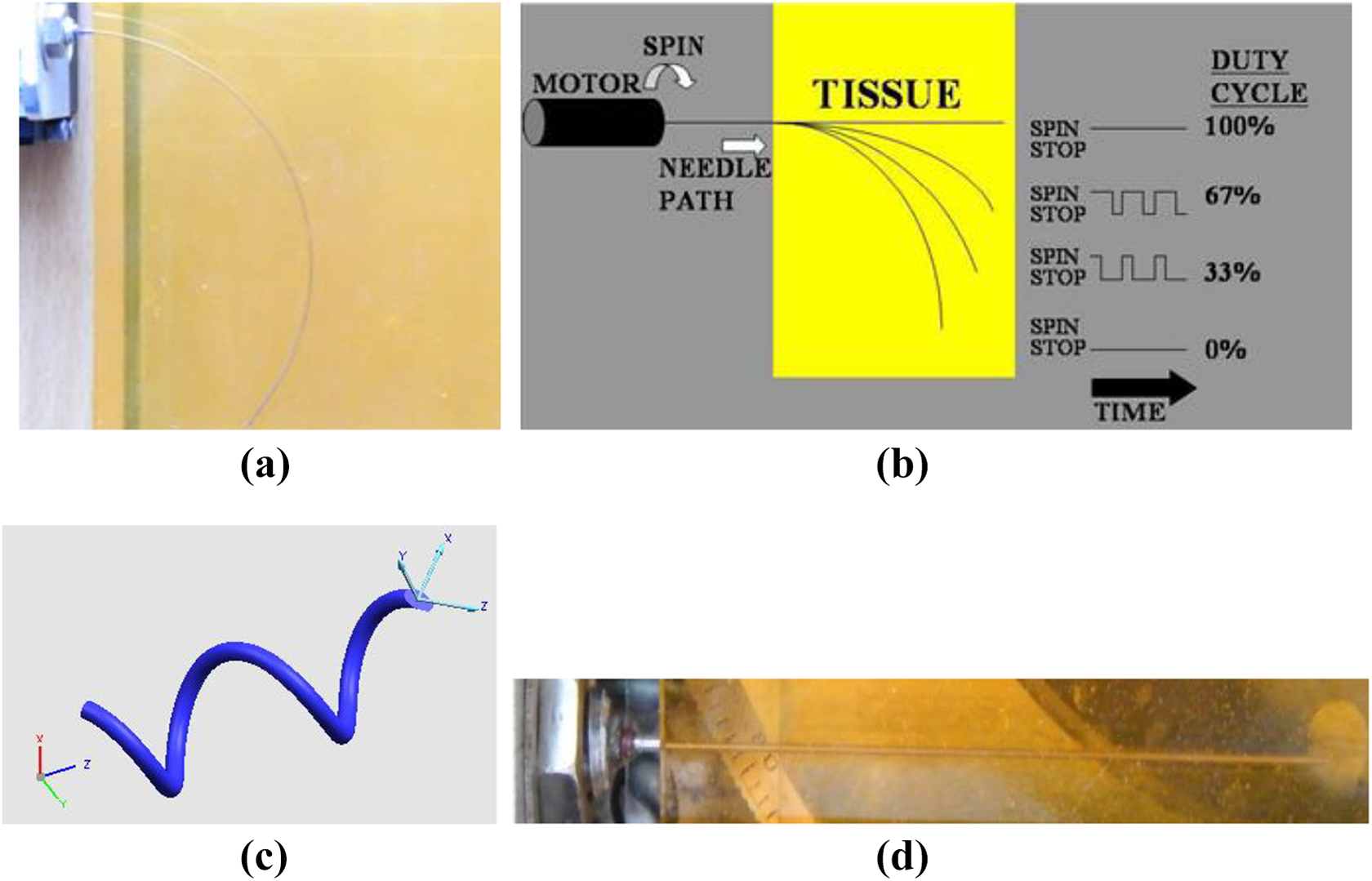
Different path forms. (a) Single arc with a constant curvature, (b) arcs with different curvatures, (c) helix, and (d) straight line.

Comparing the four path forms mentioned above, the R and the L paths are easy to obtain and easy to precisely control, while the DR and H paths need a coordinated control of insertion and rotation of the needle, thus they are with a high control cost, meanwhile they are difficult to realize a precise control. Comprehensively, R and L paths are adopted in the path optimization in this article. According to the motion characteristic, the needle motion is subjected to its kinematics, that is, the path must be smoothly connected by R and/or L, which could be combined to realize complex 3-D paths. Thus, we adopt a combination of R + L/R + R/L…or L + R + L/R…to optimize the insertion path in an environment with obstacles. Note that the L + L path is not allowable, because it happens to be a cusp in the connection of two lines, which is infeasible for the flexible needle.

Generally speaking, before inserting a segment, there is a need to adjust the orientation of the bevel tip to realize a specific configuration. And the adjustment control of bevel tip is defined as “control degree” (denoted as N). Thus, the control degree can be measured by the number of segments, N = 1, 2, 3,…. Because of the existing of the friction between the needle shaft and the tissue, it is difficult to achieve a precise rotational angle of the needle tip.²² Thus, it is necessary to reduce the control degree N.

Moreover, path form and kinematic calculation have relationship with the control degree N, as shown in Table 1.

Table 1.

Path forms under different control degrees.

N	Path forms (arc path: R, linear path: L)
1	L, R
2	LR, RL, RR
3	LRR, LRL, RLR, RRL, RRR
4	There are eight kinds of path forms.
…	…

Because different forms of paths lead to the different kinematics, the optimization calculation could not be implemented unless the path form is determined. Thus, we can divide the path forms according to the control degrees, then calculate the optimal path under the same control degree by using “path classification” method, and obtain the overall optimal path under all control degrees by using “player killing” method. We can designate a certain or a few path forms, or designate a certain or a few control degrees, or even we can also designate all the path forms or control degrees when optimization calculation is performed.

Kinematics of flexible needle

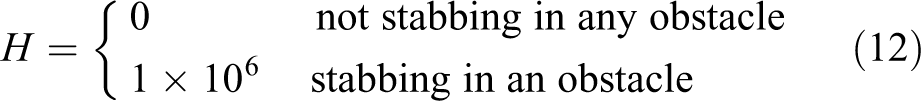
The trajectory of the flexible needle accords with the improved unicycle model,⁵ as shown in Figure 3.

Figure 3.

Improved unicycle kinematic model.

In the world frame A and the object frame B, the homogeneous transformation matrix of frame B relative to frame A is defined as

g_{a b} = [\begin{matrix} R_{a b} & p_{a b} \\ 0 & 1 \end{matrix}] \in S E (3)

where $R_{a b} \in S O (3)$ and $p_{a b} \in R^{3}$ are the rotation matrix and the position of the frame B relative to the frame A, respectively. SO(3) is a 3-D rotation group; SE(3) is a special Euclidean group, $S E (3) \subset R^{4 \times 4}$ .

The expression can be formulated in an exponential form

g_{w n} (t) = g_{w n} (0) exp (\hat{ξ} t)

where t is the execution time; $g_{a b} (0)$ is the initial configuration; ξ is a twist, $ξ \in R^{6}$ ; $\hat{ξ} \in s e (3)$ , $s e (3) \subset R^{4 \times 4}$ is a Lie algebra of the special Euclidean group.

When only the input u ₁ is executed (u ₂ = 0), the needle generates an arc, and the item in equation (1) can be formulated as

g_{r} (t) = exp ({[\begin{matrix} e_{3} \\ e_{1} / r \end{matrix}]}^{^} u_{1} t)

where ⁁ is the wedge operator to transform a vector of R⁶ into a matrix of se(3); e ₁ and e ₂ are the unit vector, $e_{1} = {[\begin{matrix} 1 & 0 & 0 \end{matrix}]}^{T}$ and $e_{3} = {[\begin{matrix} 0 & 0 & 1 \end{matrix}]}^{T}$ .

When only the input u ₂ is executed (u ₁ = 0), the needle rotates about the z-axis, and the item $exp (\hat{ξ} t)$ in equation (1) can be formed as

g_{z} (t) = [\begin{matrix} cos u_{2} t & - sin u_{2} t & 0 & 0 \\ sin u_{2} t & cos u_{2} t & 0 & 0 \\ 0 & 0 & 1 & 0 \\ 0 & 0 & 0 & 1 \end{matrix}]

When the inputs u ₁ and u ₂ are executed at the same time, and u ₂ ≥ 5u ₁, the path of the needle is a straight line along the insertion direction, and the item $exp (\hat{ξ} t)$ in equation (1) can be calculated as

g_{l} (t) \approx g_{z l} (t) g_{z} (t), (u_{2} \geq 5 u_{1})

where g _zl (t) is the homogeneous transformation matrix of translation along the z-axis.

g_{z l} (t) = [\begin{matrix} I_{3 \times 3} & d e_{1} \\ 0_{1 \times 3} & 0 \end{matrix}]

For the improved unicycle kinematic model considering the deflection ϕ and the rebounds b (b ₁, b ₂, b ₃), the kinematics of the needle for different path forms are as follows

g_{a b} (T) = {\begin{matrix} g_{a b} (0) g_{r} (T_{1} - b_{1} / u_{1}) g_{z l} (b_{1} / u_{1}) g_{z} (π / u_{2}) g_{r} (T_{2}) \dots, RR \dots \\ g_{a b} (0) g_{r} (T_{1} - b_{2} / u_{1}) g_{z l} (b_{2} / u_{1}) g_{l} (T_{2}) \dots, RL \dots \\ g_{a b} (0) g_{l} (T_{1} - b_{3} / u_{1}) g_{r} (T_{2} + b_{3} / u_{1}) \dots, LR \dots \end{matrix}

where T is the total execution time; T_i is the execution time of the ith segment, $T = \sum_{i = 1}^{n} T_{i}$ ; g _ab (0) is the initial configuration of the needle, for the path with the first segment of an arc, g _ab (0) is the homogeneous transformation matrix of rotation ϕ about the z-axis, $g_{a b} (0) = g_{x} (ϕ) = [\begin{matrix} 1 & 0 & 0 & 0 \\ 0 & cos ϕ & - sin ϕ & 0 \\ 0 & sin ϕ & cos ϕ & 0 \\ 0 & 0 & 0 & 1 \end{matrix}]$ , while for the path with the first segment of a line, g _ab (0) is a fourth order unit matrix, $g_{a b} (0) = I_{4}$ ; b ₁, b ₂, and b ₃ are the rebound for RR, RL, and LR, respectively. Details are available in the study by Zhao et al.⁵

In addition, considering the optimization of the needle insertion posture, it is necessary to add two parameters of the needle insertion angles, which are θ ₁ (rotation angle about the x-axis of the frame B) and θ ₂ (rotation angle about the z-axis of the frame B), as shown in Figure 4.

Figure 4.

Path planning considering needle insertion posture.

Therefore, the whole kinematics is as follows

{\tilde{g}}_{a b} = g_{x} (θ_{1}) g_{z} (θ_{2}) g_{a b}

where $g_{x} (θ)$ and $g_{z} (θ)$ are the homogeneous transformation matrix of rotation about the x-axis and z-axis, respectively.

Path optimization algorithm

Establishment of objective function

The aim of the path optimization algorithm is to find the optimal path which is the shortest, the safest, able to avoid the obstacles, and with the least control cost, while considering the insertion posture. The optimization parameters are the insertion posture θ (θ ₁, θ ₂) and the control inputs u (u ₁, u ₂). Thus, the optimization objective function is established as follows

min F (θ, u, T) = min {α_{1} L + α_{2} D + α_{3} H + α_{4} N}

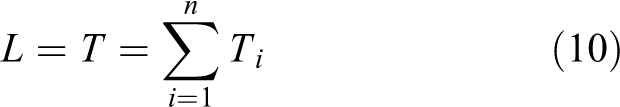
where T is the total execution time; L is the length of the path; D is the risk degree of the path, which measures the degree of the risk (or on the contrary, the safety) of the path; H is the punishment degree, which will take effect if the needle stabs in an obstacle; N is the control degree; α ₁–α ₄ are the weighting coefficients of the objective function.

Realization of sub-objective functions

The first item of the objective function is the length of the whole path. In a simulation, it is reasonable to set $u_{1} (t) \equiv 1$ , so the length of the path equals the execution time of the needle, which is the summation of individual execution time of each segment

L = T = \sum_{i = 1}^{n} T_{i}

The second item is the risk degree, which is defined as a function of the shortest distance between the path and each obstacle. The smaller the D gets, the safer the path is

D = {\begin{cases} 0 without obstacles \\ \sum {0.1}^{d_{i}} with obstacles \end{cases}

where d_i is the shortest distance between the path and the ith obstacle, $d_{i} = min (| | p_{n o_{i}} | | - r_{o_{i}})$ , where o and r are the origin and radius of a circle, respectively, which represents an obstacle, and n is a point in the path.

The third item is the punishment degree, the value of which will be zero if the needle does not stab in any obstacle, while will be an enormous one if the needle stabs in any obstacle.

H = {\begin{cases} 0 not stabbing in any obstacle \\ 1 \times 10^{6} stabbing in an obstacle \end{cases}

And the fourth item is the control degree, N = 1, 2, 3,…. The control degree with 3 is competent for a general clinical surgery, thus we can set 3 as the maximum of the control degree. However, it can be released to 4 or more if necessary.

The weighting coefficients α ₁–α ₄ can be selected based on the following robustness analysis of the optimization algorithm.

Robustness analysis of optimization algorithm

The robustness analysis of the optimization algorithm is mainly to analyze the sensitivity of the optimization results regarding to the weighting coefficients. Different from the traditional weighting coefficients, the weighting coefficients in this algorithm have their physical meanings. Taking the path length as a benchmark, the meaning of each weighting coefficient is as follows: α ₂ = a indicates that the path is allowed to be close to a particular obstacle (of course, within a safe range), however, under the same control degree as well as other coefficients, the path will be better if it saves more than a mm relative to the former; α ₃ = b is to ensure that the value of the function will be an enormous one (>b × 10⁶) if the needle stabs in the obstacles; while α ₄ = c indicates that when the control degree is increased by one, under the same risk degree and the other coefficients, the path will be considered to be better if it saves more than c mm relative to the former.

When discussing the influence of one of the weighting coefficients to the optimization function, we can allow it change within a reasonable range, while the other coefficients are assumed invariant. According to the physical meanings of the weighting coefficients, we set α ₁ ≡ 1 due to it is the benchmark, the sensitivity of which need not to be analyzed. Because the total path length is about 100 mm in a general clinical surgery, α ₂ and α ₄ are meaningless if they are with high values according to their physical meanings. And α ₃ as the penalty coefficient can be very large to ensure the penalty.

Set the start point of the needle as (0, 0, 0), the target as (0, 0, 90), the radii of the three obstacles as 10, 11, and 13 mm, respectively, and the center position as (0, 30, 50), (0, −5, 40) and (0, −40, 30), respectively. And take the discrete interval time as Δ = 0.1 s. Taking an example of a flexible needle with the tip angle of 30°, the circular arc radius is r = 63.7 mm.⁵ The optimization algorithm is programmed using sequential quadratic programming method with MATLAB® (version 7.8.0, R2009a; MathWorks, Natick, MA).

Sensitivity analysis of α ₂

Set α ₁ = 1, α ₃ = 10³, α ₄ = 2, allow α ₂ to change in a range of 1 to 10, and set the control degree as 2. When α ₂ changes from 1 to 10, effects under different values of α ₂ are as shown in Figure 5.

Figure 5.

Different effects of path optimizations under different values of α ₂. (a) α ₂ = 1 and (b) α ₂ = 10.

It can be seen from Figure 5, the larger the value of α ₂, the greater distance of the path from the obstacles, which is benefit for improving the safety of the insertion. However, if the value of α ₂ is particularly large, it will enforce the path far away from the obstacles, although the safety of the insertion is improved, the length of the path is forced to be increased, thus the value of α ₂ cannot be too large, generally 1 to 10. And the changing curve of the optimization values is shown in Figure 6. It can be seen from the figure, in the reasonable range of α ₂, the optimization result changes little. Thus, a conclusion can be drawn that the sensitivity of α ₂ is very low to the objective function.

Figure 6.

Optimization results under different values of α ₂.

Sensitivity analysis of α ₃

Set α ₁ = 1, α ₂ = 1, α ₄ = 2, and α ₃ is changed in a range from 1 to 10⁹. The bevel tip angle is also 30°, and the control degree is also 2. The changing curve of the optimization values is shown in Figure 7.

Figure 7.

Curve of optimization results under different values of α ₃.

It can be seen that the optimization result is stable with the change of α ₃, which is reasonable because when the needle does not stab in any obstacle, this item always equals zero. The only difference is that when the needle stabs in an obstacle, the value of optimization function will be varied. Thus, the sensitivity of α ₃ to the objective function is null.

Sensitivity analysis of α ₄

Set α ₁ = 1, α ₂ = 1, α ₃ = 10³, and α ₄ is changed from 0 to 10. The optimization result changes are shown in Table 2.

Table 2.

Optimization results of different values of α ₄.

α ₄	Optimal path form	Corresponding control degree N
0–0.66	LRL	3
0.67–8.11	RL	2
8.12–10	R	1

From the results, it can be seen that α ₄ is the switch of the forms of the optimal path, which directly influences the role of the control degree played in the objective function. Since the control degree directly influences the quality of the path, it should be made a full use. It can be seen from Table 2, the value of α ₄ will affect the form of optimal path and the control degree, and thus it is critical and crucial that the values of α ₄ should be appropriately selected.

The viewpoint in this article holds that the optimal path is RL with the control degree of 2 (details are available in the next section). Therefore, from the results in Table 2, the range of α ₄ should be set from 1 to 8. The optimization results are shown in Figure 8.

Figure 8.

Curve of optimization results under different values of α ₄.

It can be seen that although the function value linearly increases with the increase of α ₄, the length of the optimal path remains stable, as shown in Figure 8. Moreover, the path always remains in the form of RL, thus the sensitivity of α ₄ to the objective function is very low.

In summary, the sensitivities of the weighting coefficients are all very low to the optimization objective function. Thus, the optimization objective function is stable and with strong robustness regarding to all weighting coefficients.

Simulation and discussion

The simulation condition is the same as above. And set α ₁ = α ₂ =1, α ₃ =10³, α ₄ =2. Here, we set the obstacles as circles in order to simplify the optimization calculation. As for the irregular obstacles, they could be replaced by circles through the following three methods according to their complexity: (1) Circumscribed circle: the obstacle is replaced by a circumscribed circle, which is suitable for the regular obstacles, as shown in Figure 9(a); (2) segmented circles: the obstacle is segmented by a few circles to envelope the whole obstacle, which is appropriate for the irregular but without large cusp or sunken obstacles, as shown in Figure 9(b); (3) bordered circles: the edge of the obstacle is enveloped by a series of small circles to border the edge of the obstacle, which is applicable for the very irregular obstacles, as shown in Figure 9(c).

Figure 9.

Circle replacement method of the obstacles. (a) Circumscribed circle, (b) segmented circles, and (c) edged circles.

Moreover, the abovementioned methods can be combined to replace the obstacles. And the rule is to guarantee to envelope all the obstacles with fewer circles, which is better for the optimization calculation. Thus, the proposed path optimization algorithm has a universality, which fits for any kinds of obstacles.

The simulation results are obtained as follows: the optimal path with the control degree of 1 is R, as shown in Fig. 10(a). There is no solution for L form, because in the presence of obstacles, the needle cannot directly reach the target with a linear path. The optimal solutions for three different forms with the control degree of 2 are shown in Figure 10(b), therein the best one is RL, which is also the optimal path of the whole, as shown in Figure 10(c). The optimal solutions for five different forms with the control degree of 3 are shown in Figure 10(d), therein the best one is LRL, as shown in Figure 10(e). The optimization results of each form of paths are shown in Table 3.

Figure 10.

Path optimization results of path forms. (a) When N = 1, the optimal solution is R; (b) optimization solutions for three forms of paths when N = 2; (c) when N = 2, the optimal solution is RL, which is also the overall optimal solution; (d) optimization solutions for five forms of paths when N = 3; and (e) when N = 3, the optimal solution is LRL.

Table 3.

Comparison of optimal paths in different forms.

Path form	Optimization function value	Total length of path (mm)		Rotation angle of needle tip (°)	Length of the first segment (mm)	Rotation angle of needle tip (°)	Length of the second segment (mm)	Rotation angle of needle tip (°)	Length of the third segment (mm)
Path form	Optimization function value	Total length of path (mm)	Rotation angle about x-axis (°)	Rotation angle of needle tip (°)	Length of the first segment (mm)	Rotation angle of needle tip (°)	Length of the second segment (mm)	Rotation angle of needle tip (°)	Length of the third segment (mm)
R	101.5386	99.54	−46.3	0	99.54	—	—	—	—
RL	95.4422	91.43	−29.0	0	43.03	0°	48.40	—	—
LRL	96.7624	90.77	−9.8	0	32.90	0°	19.83	0°	38.04

As shown in Figure 10 and Table 3, a conclusion can be drawn that (1) the optimal path of each control degree contains the linear path (except for R), because the linear path can shorten the length of path effectively; and (2) the form of RL is the overall optimal path (the value of the optimization function is the least), because on the one hand, although the control degree of R is the smallest and it is easy to control, it has the longest path, thus it cannot be the optimal path on the other hand, although the control degree of RL increases by 1, accordingly the control difficulty is increased, the length of path is much shorter (8.11 mm shorter) than that of R, thus it is better compared to R and as for LRL, although the length of path is a little shorter (0.66 mm shorter) than that of RL, it increases one control degree, which makes the path form complex and difficult to control precisely, resulting that the overall value of the function is increased. Thus, RL is the optimal path on the whole.

In order to reveal the priority of the proposed algorithm, we compared it with the commonly used RRT-based algorithm in the same conditions. The step size is 10 mm, and the tolerance (i.e. the allowance between the needle tip and the target) is 1 mm. The optimal result is shown in Figure 11, if it is valued by the same standard as our proposed algorithm, and the comparison of both best paths generated by the two algorithms is shown in Table 4.

Figure 11.

Path planning result of the RRT-based algorithm.

Table 4.

Comparison of optimal paths of both algorithms.

Algorithm	Optimization function value	Total length of path (mm)	Contol degree
Our proposed agorithm	95.4422	91.43	2
RRT-based agoirthm	101.8523	91	5

RRT: rapidly exploring random trees.

Through the comparison of the two paths, the path calculated by our proposed algorithm is better in light of the optimization function value. Although the length of the path generated by the RRT-based algorithm appears a little shorter, actually it is with the tolerance of 1 mm to the target. As a matter of fact, its whole path would be longer (if it reached to the target), and meanwhile with a poor accuracy and a high control cost (control degree). Thus, we conclude that the path of our proposed algorithm is overall superior to the RRT-based one.

Experimentation

We chose three typical paths for experimentation: R with the control degree of 1, RL with the control degree of 2, which is also the optimal path overall, and LRR with the control degree of 3. The realization of the three paths can prove the feasibility of various forms of paths. Experimental results are shown in Figure 12, the comparison between the experimental and theoretical paths is shown in Figure 13 (90° clockwise rotation compared to the experimental directions).

Figure 12.

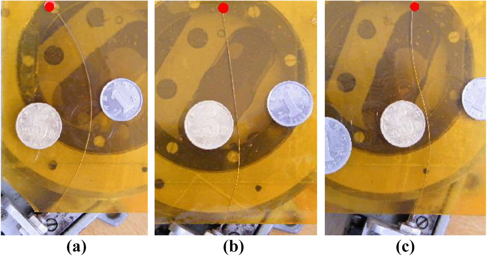
Experimental results. (a) Form of R, (b) form of RL, and (c) form of LRR.

Figure 13.

Experimental and theoretical paths of the proposed algorithm.

From the comparison between the experimental and theoretical paths, it can be concluded that not only the paths with various forms can be implemented well but also the experimental paths fit the theoretical ones well. The mean square root of the errors is 0.90, and the higher of the control degree, the larger of the errors. The maximal error is 1.48 mm appearing at the end of the LRR, which is reasonable as the control degree increased. The experimental results not only verify the feasibility of the path optimization algorithm but also prove realization of the various forms of paths, moreover, prove the rationality of reducing the control degree.

We also performed the experiment for the RRT-based path in order to make a comparison. The result is shown in Figure 14.

Figure 14.

Experimental and theoretical paths of the RRT-based algorithm. RRT: rapidly exploring random trees.

The results show that the accuracy of the RRT-based path is much inferior to RL path. It is because RL is easy to realize with less control degree, while the other is the opposite. More control degrees will cause more uncertainties and errors, which proves the rationality of reducing the control degree again.

Conclusion

On the basis of kinematics calculation of the flexible needle, and considering the injury on the patient, risk of insertion and difficulty of control, a multiple objective optimization function is established, and a path optimization is carried out in a 2-D environment with obstacles. The physical meanings of the weighting coefficients for the optimization objective function are proposed. The value ranges of the weighting coefficients for a general clinical surgery are determined, and the sensitivities of the weighting coefficients to the optimization objective function are analyzed. According to the physical meanings of the weighting coefficients, the overall optimal path in the simulation results are analyzed and explained, and the experimental verification and comparison with the RRT-based algorithm are carried out.

The results show that:

The proposed optimization algorithm is able to calculate optimal path, which proves superior to the RRT-based path;

The optimization function has low sensitivity to all the weighting coefficients, thus the optimization algorithm has strong robustness.

According to the analysis of the simulation results, the obtained optimal path is reasonable and correct, which proves the rationalities of the physical meanings of the weighting coefficients.

The accuracy of the experiment is within 2 mm, which meets the needs of a general clinical surgery, and the maximal error will always appear at the end of the path with the highest control degree, which proves that it is reasonable to consider reducing the control degree.

Footnotes

Declaration of conflicting interests

The author(s) declared no potential conflicts of interest with respect to the research, authorship, and/or publication of this article.

Funding

The author(s) disclosed receipt of the following financial support for the research, authorship, and/or publication of this article: This research is supported in part by the National Natural Science Foundation of China (grants #51305107 and #51675142) and by the Natural Science Foundation of Heilongjiang Province of China (grant #ZD2018013).

ORCID iD

Yan-Jiang Zhao

References

Podder

Dicker

Hutapea

. A novel curvilinear approach for prostate seed implantation. Med Phys 2012; 39(4): 1887–1892.

Webster

III RJ

Kim

Cowan

. Nonholonomic modeling of needle steering. Int J Robot Res 2006; 25(5–6): 509–525.

Gao

Zheng

. A finite element approach for simulating soft tissue deformation during needle insertion. J Comput Aid Des Comput Graph 2009; 21(11): 1601–1605.

Jiang

Wang

. Mechanics-based interactive modeling for medical flexible needle insertion in consideration of nonlinear factors. J Comput Nonlin Dyn 2016; 11(1): 1–11.

Zhao

Zhang

Shao

. Kinematic modeling and experimental study of flexible needle. Robot 2010; 32(5): 666–673.

Alterovitz

Patil

Derbakova

. Rapidly-exploring Roadmaps: weighing exploration vs. refinement in optimal motion planning. In: Proceedings of the IEEE international conference on robotics and automation, Shanghai, China, 9–13 May 2011, pp. 3706–3716. IEEE.

Duindam

Goldberg

. Motion planning for steerable needles in 3D environments with obstacles using rapidly exploring random trees and backchaining. In: Proceedings of the IEEE international conference on automation science and engineering, Arlington, VA, USA, 23–26 August 2008, pp. 41–46. IEEE.

Patil

Alterovitz

. Interactive motion planning for steerable needles in 3D environments with obstacles. In: Proceeding of the IEEE RAS/EMBS international conference biomedical robotics and biomechatronics, Tokyo, Japan, 26–29 September 2010, pp. 893–899. IEEE.

Patil

Burgner

Webster

III . Needle steering in 3-D via rapid replanning. IEEE Trans Robot 2014; 30(4): 853–864.

10.

Vrooijink

Abayazid

Patil

. Needle path planning and steering in a three-dimensional non-static environment using two-dimensional ultrasound images. Int J Robot Res 2014; 33(10): 1361–1374.

11.

Bernardes

Adorno

Borges

. 3D robust online motion planning for steerable needles in dynamic workspaces using duty-cycled rotation. J Control Autom Elect Syst 2014; 25(2): 216–227.

12.

Xiong

. Path planning for flexible needle based on environment properties and random method. Comput Eng Appl 2017; 53(16): 121–125, 160.

13.

Zhao

Huang

. Motion planning of the cannula flexible needle based on the improved RRT algorithm. Chinese J Sci Instrum 2017; 38(3): 620–628.

14.

Alterovitz

Branicky

Goldberg

. Motion planning under uncertainty for image-guided medical needle steering. Int J Robot Res 2008; 27(11–12): 1361–1374.

15.

Park

Wang

Chirikjian

. The path-of-probability algorithm for steering and feedback control of flexible needles. Int J Robot Res 2010; 29(7): 813–830.

16.

Duindam

Alterovitz

Sastry

. Screw-based motion planning for bevel-tip flexible needles in 3D environments with obstacles. In: Proceedings of the IEEE international conference on robotics and automation, Pasadena, CA, USA, 19–23 May 2008, pp. 2483–2488. IEEE.

17.

Zhao

Zhang

. Reverse Path Planning for Flexible Needle in 2D Soft Tissue with Obstacles. In: 2nd International conference on frontiers of manufacturing and design science, Taichung, Taiwan, 11–13 December 2011, pp. 4132–4137. Trans Tech Publications.

18.

Huo

Zhao

Han

. Puncture path planning for bevel-tip flexible needle based on multi-objective particle swarm optimization algorithm. Robot 2015; 37(4): 385–394.

19.

Zhang

Zhao

. Modeling of bevel-tipped needle inserting into soft tissue and estimation of needle tip trajectory. Chinese J Sci Instrum 2015; 36(8): 1744–1751.

20.

Minhas

Engh

Fenske

. Modeling of needle steering via duty-cycled spinning. In: Proceeding of the international conference IEEE engineering in medicine and biology society, Lyon, France, 22–26 August 2007, pp. 2756–2759. IEEE.

21.

Majewicz

Siegel

Stanley

. Design and evaluation of duty-cycling steering algorithms for robotically-driven steerable needles. In: IEEE international conference on robotics & automation, Hong Kong, China, 31 May–5 June 2014, pp. 5883–5888. IEEE.

22.

Reed

Okamura

Cowan

. Controlling a robotically steered needle in the presence of torsional friction. In: IEEE international conference on robotics and automation, Kobe, Japan, 12–17 May 2009, pp. 3476–3481. IEEE.

Path optimization algorithm and its robustness for bevel tip flexible needle

Abstract

Keywords

Introduction

Kinematic analysis of bevel flexible needle

Path form analysis

Kinematics of flexible needle

Path optimization algorithm

Establishment of objective function

Realization of sub-objective functions

Robustness analysis of optimization algorithm

Sensitivity analysis of α 2

Sensitivity analysis of α 3

Sensitivity analysis of α 4

Simulation and discussion

Experimentation

Conclusion

Footnotes

Declaration of conflicting interests

Funding

ORCID iD

References

Sensitivity analysis of α ₂

Sensitivity analysis of α ₃

Sensitivity analysis of α ₄