
Abstract
High-speed press lines are related to the fierce competition in the automobile industry and rely on continuous high-efficiency automated feeding systems. Kinematic simulation systems have facilitated the improvement of production processes by generating real-time kinematic curves to avoid interference in feeding systems. In this article, a new method based on quintic polynomials in MATLAB and ADAMS is introduced to achieve whole-line planning using a kinematic simulation system for path planning. Furthermore, secondary interface is developed to visualize the kinematic curves and animate the generated whole-line trajectories. The kinematic simulation system was found to improve the efficiency of generating predicted trajectories in joint or Cartesian space and achieved reliable whole-line path planning, including collision inspection and singular point detection, by using parametric modeling and analyzing kinematic curves. Finally, the kinematic simulation system was verified using results of a kinematic analysis and example simulation.
Keywords
Introduction
Path planning is an important part of kinematic simulation systems. For a high-speed press line automated feeding system, the tools fixed to the end-effector of a manipulator are used to move stamping parts from one press to another following a particular path in Cartesian space. To complete a given task, motion trajectories of the tools must satisfy the limits of certain performance indices, such as minimum traveling time, minimum energy, or minimum jerk (time rate of change of acceleration).
To date, a number of methods have been developed for path planning, both in Cartesian space and joint space. Kucuk used an optimal trajectory generation algorithm to predict minimum-time smooth motion trajectories for serial and parallel manipulators. 1 Chen et al. presented a method based on Hamilton–Jacobi theory for computing energy-optimal trajectories of a two-link planar manipulator. 2 To optimize robot path planning for welding complex joints, Fang et al. selected solutions that produce minimum joint movement. 3 Although these methods are quite effective in acquiring improved trajectories, they are not computationally practical and cannot be used for complex nonlinear systems. Thus, a number of nontraditional methods have been introduced to generate solutions under suboptimal conditions. The algebraic method developed by Zhang et al. for trajectory planning was shown to save time. 4 Furthermore, Mahil and Al-Durra attempted to linearize the mathematical model of a two-degree of freedom (2-DOF) robotic arm, which was a highly dynamic nonlinear system. The novel method for solving robot trajectory problems was shown to be extremely effective for this type of robot. 5 To improve these results, more complex algorithms including cubic and quintic polynomials have been proposed to generate the optimum path. 6 A path planning method was proposed by Hu et al. that combined polynomial interpolation with Newton interpolation, and was shown to offer improved mathematical descriptions requiring fewer calculations. 7 Xu et al. presented a cost function that took into account dynamic equations as well as velocity, acceleration, jerk, and torque constraints. 8 The customized cost function was used to achieve more accurate trajectories by balancing the traveling time and mechanical energy of the manipulator while considering particular constraints. Intelligent algorithms have also been used in this field. Das et al. used hybridization of a particle swarm optimization with an improved gravitational search algorithm to determine the optimal trajectory for multiple robots in a cluttered environment, and demonstrated the superiority compared to other algorithms. 9 Using simulated annealing, Tavares et al. reduced the number of configuration parameters and improved the efficiency of acquiring an ideal robot path. 10
In addition to path planning, kinematic simulation systems are crucial for optimizing path planning of multi-joint robots and to achieve accurate and smooth paths under various constraints, including displacement, velocity, and acceleration. Two common types of simulation system exist: dynamic simulation systems and kinematic simulation systems. Dynamic simulation ignores secondary factors and generates an approximation model. However, large errors can occur in practical applications. The high accuracy of kinematic equations means kinematic simulations are more reliable and results are shown to be relatively consistent with real situations. Therefore, a number of simulation systems based on kinematic path planning have been developed. Cui et al. studied the kinematic model and experimental system of a telescopic excavator and achieved autonomous operation using SimMechanics software. Moreover, results of the simulations were consistent with experimental results. 11 To calculate the DOF of a mechanism consisting of two translations and one rotation, Lin et al. used screw theory to verify the model and created a kinematic model based on a co-simulation in SolidWorks and MATLAB. 12 In addition, several complex robot models have been developed and simulated. Yu et al. simulated the motion of a revolute, prismatic and spherical (3-RPS) kinematic pair parallel robot using SimMechanics and Simulink and obtained kinematic data and motion animations for observing the robotic path development. 13 Michel developed a mobile robot simulation software to create control programs via robotic libraries that were transferred to several commercially available real mobile robots, which was extremely useful for both teaching and research. 14 In addition, simulations have been used to select the best method for obtaining a robot trajectory. Cai used customized software to develop a 6R industrial robot simulation system and results of the radial basis function neural network algorithm were capable of accurate robot trajectory planning. 15 Gouasmi et al. modeled and simulated two different rotary robot types and compared their postures in SolidWorks and MATLAB/Simulink software to successfully verify their theoretical model. 16
In this article, a quintic polynomial function was used for trajectory planning in both the Cartesian and joint space to ensure continuous velocity and acceleration. Compared to other methods, path planning based on the quintic polynomial method was found to be superior. The quintic polynomial method not only inherits the advantages of cubic spline optimization, 17 but also reduces vibration by independently tuning acceleration, which offers better way than cubic spline optimization with input shaping. 18 A user interface was developed to clearly visualize the tooling path in real time using parameterization. In addition, a kinematic simulation system of a high-speed press line automated feeding robot was developed and kinematic simulations were realized. Benefits of the system include ease of operation by nonexperts and effective improvements in the optimization of trajectory planning for high-speed press line automated feeding robots. In brief, this article provides an efficient way of combining path planning methods based on quintic polynomial and co-simulation in MATLAB (version 2012b) and ADAMS (version 2013) with kinematic simulations for the automobile industry to generate paths and whole-line relationships using parametric modeling.
This article is organized as follows: kinematic analysis of the high-speed press line automated feeding manipulator is introduced in the second section; in the third section, the kinematics simulation system is developed based on an example simulation, including modeling of the mechanical system, model simulation, development of a customized user interface, and analysis of the kinematic curves; finally, some conclusions are summarized in the fourth section.
Kinematics analysis of high-speed press line automated feeding manipulator
Path planning method
The diagram and solid structure of the 2-DOF redundant automatic feeding robot are shown in Figure 1. The system consists of rods R1, R2, R3, and R5, sliders D4 and D7, and handles R6. Rod R1 is connected to a fixed base. The relationship between neighboring joints is ensured by means of the Denavit–Hartenberg (D-H) convention. However, to obtain the inverse kinematic solutions, a new method is proposed for a 2-DOF redundant multi-joint robot since traditional methods are difficult to implement, especially for redundant robots.
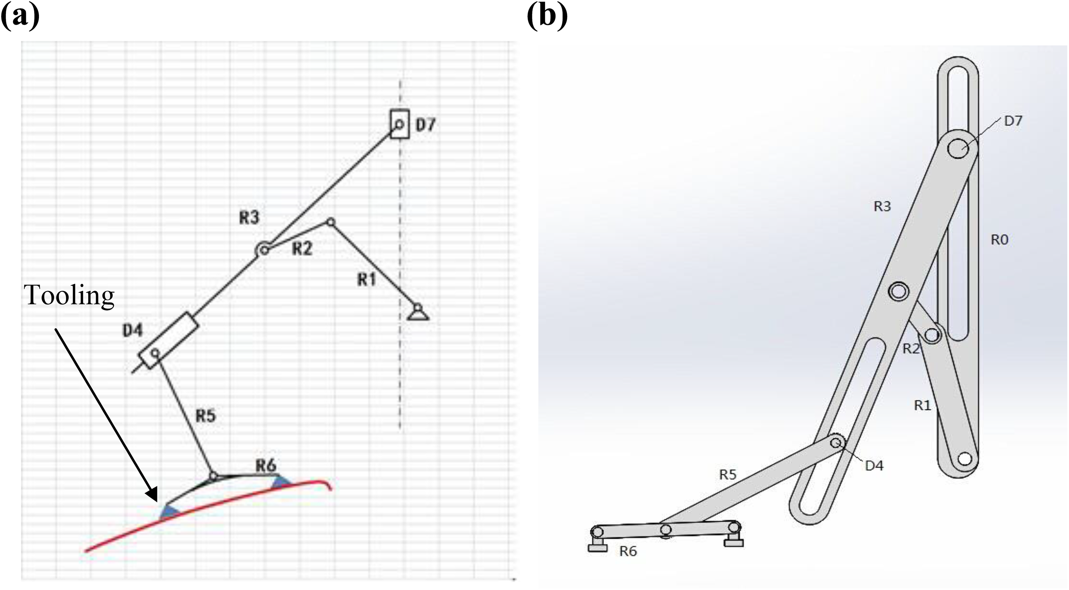
Automated feeding robot. (a) Diagram of automated feeding robot and (b) solid structure of automated feeding robot.
The tooling path is attached to robotic joint R6; therefore, a combination of curves including displacement, velocity, and acceleration in the x- and y-direction must be generated in Cartesian space and several segments of the curves can be planned in the x- and y-direction using a quintic polynomial. It can be noted that the combined points of the tooling path in the XY space can be regarded as the combination of simultaneous positions in the x- and y-direction. If acceleration is known, velocity and displacement can be derived by integration. Based on this idea, kinematic curves of the tooling and redundant joints are easily obtained. Then, the kinematic curves of additional joints can be determined based on the D-H convention. Thus, general equations are deduced and regarded as internal algorithms of the kinematic simulation system. Moreover, continuous kinematic parameters, including velocity, acceleration, and jerk, are necessary for generating a smooth path.
The tooling path attached to the robotic center of mass of joint R6 (R6.cm) in Figure 1 was used as an example. As shown in Figure 2(a), the path of manipulator in Cartesian space can be divided into several segments, which are waiting time (segment ①), loading move-in and move-out (segments ③ and ⑤), unloading move-in and move-out (segments ⑦ and ⑨), loading and unloading time (segments ④ and ⑧), and running with material and running without material (segments ②, ⑥, and ⑩). Then, the path of every segment can be decomposed into two components along the x- and y-axis. Further, segments ②, ③, ⑨, and ⑩ can be merged in the x-direction to reduce the amount of computation involved. The solid structure of the presses and molds are shown in Figure 2(b) and manipulators are situated between neighboring presses.

Whole-line arrangements of automated feeding system. (a) Schematic of tooling path and (b) solid structure of presses and molds.
Assuming acceleration a of an arbitrary section in any direction can be expressed as

where t is time and b, c, d, and e are constants.
Integrating equation (1) once or twice, velocity v and displacement s can be obtained, respectively, and are given by

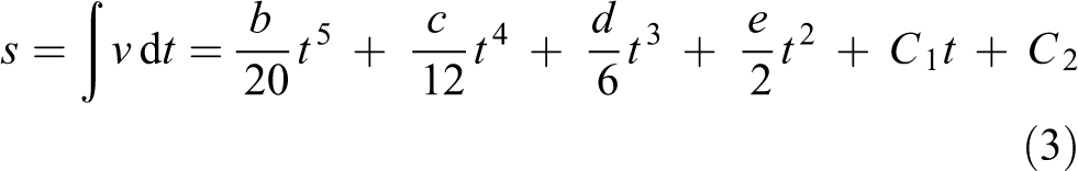
where C 1 and C 2 are constants determined by the initial and final conditions.
The path can be divided into several segments. Along each segment, velocity and acceleration values are zero at the initial and final time. It is beneficial to obtain general kinematic equations and run smoothly at the meeting point between neighboring sections. The constraints are given as follows


Based on the abovementioned constraints, equations (1) to (3) can be further solved using the substitution method, elimination method, and Shengjin’s formula, respectively, and then are given as

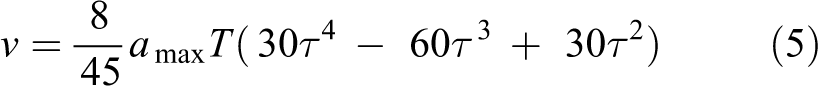

where
To generate the tooling path, the running time of every segment must be known such that equations (4) to (6) can be solved. The method of “equal division of time and matching of movements” can be used to determine the time. 19 The time required to complete each segment should be an integral multiple of the time interval. Next, the loading and unloading positions are configured and values of the loading move-in and move-out height (positions I and III in Figure 2) and unloading move-in and move-out height (positions II and IV in Figure 2) are input into the model. Subsequently, the displacement, acceleration, and velocity of each segment are calculated using equations (4) to (6), respectively, and maximum values are considered to be the maximum values of the entire path. The path is generated in the x- and y-direction. Therefore, the complete tooling path is also generated in the Cartesian space.
In this article, detailed steps of the path planning process in Cartesian space and joint space are as follows:
Step 1: Tooling paths in Cartesian space are divided into several segments in the x- and y-direction, as shown in Figure 2(a). Meeting points between neighboring sections in the same direction are subjected to the same kinematic constraints when velocity and acceleration are zero. Equations (4) to (6) are used as the general equations and internal algorithm in the kinematic simulation.
Step 2: Based on actual displacements in the x- and y-direction, data are input into the path-planning interface, shown in Figure 3, to generate the tooling paths.

Path-planning interface.
Step 3: If redundant manipulators exist, the same method is applied for path planning of redundant joints. Otherwise, paths of other joints in the joint space are determined by the D-H convention.
Example simulation
In the example simulation, the distance between presses was 6 m and maximum acceleration was 3g and g where g is 9.8 m/s2 in the x- and y-direction, respectively, based on the selected motors. The user interface displays actual data, which can be used to examine the effectiveness of the proposed method. The path-planning interface was built in MATLAB, as shown in Figure 3. Press line speed was 12 strokes per minute (SPM), such that each press line stamps 12 times per unit time, loading move-in and unloading move-out heights were both 150 mm, and loading move-out and unloading move-in heights were 430 mm. When data were input and the “plot” button was pressed, the path was generated.
As mentioned earlier, every joint is subjected to independent displacement, velocity, and acceleration constraints. At the end of the simulation, trajectories of the manipulator were determined, and trajectories of the slider D4 and handle R6, which were the redundant joints in this article, can be determined in the same way. Therefore, trajectories of other joints can be determined by the D-H convention.
Paths based on the data presented in Figure 3 are shown in Figure 4. The path parameters including displacement, velocity, and acceleration in the x- and y-direction are shown in Figure 4(a) to (d). It can be observed that the paths are smooth and accelerations are not greater than maximum values. Furthermore, tooling paths for different move-in and move-out heights are shown in Figure 5. The final two curves depict velocity and acceleration at a press line speed of 15 SPM. The rest of the data were input into the model as previously, and trends of velocity and acceleration are shown to be the same, however, waiting time is reduced. Therefore, different paths are generated accurately and efficiently based on different inputs adapted to different press lines.

Model of 430/150 mm move-in and move-out heights. (a) Tooling path, (b

Comparative curves for different input data.
Development of kinematic simulation system
To establish parametric models of mechanical systems, ADAMS uses an interactive graphical environment. Bodies, connectors, and forces were provided within the ADAMS software environment, and modules were obtained from third-party software manufacturers in order to quickly obtain kinematic results using the ADAMS solver. The framework of the kinematic simulation system included four subprocesses: modeling of the mechanical system, model simulation, developing the customized user interface, and analyzing the kinematic curves. Here, the kinematic simulation system proposed in this article was only applied to the press line automated feeding system relevant to the automobile industry.
Modeling of mechanical system
During the modeling process, a three-dimensional model of the mechanical system was first created and assembled in SolidWorks (version 2012) and then introduced into ADAMS. Modeling was based on the common Parasolid type, which can be used to maintain the original position relationships while ignoring constraints. Relative positions between the presses and feeding manipulators were adjusted to create a complete model of all press lines. For example, the position including feeding distance in the x-direction and the distance of the loading point in the y-direction, as well as the waiting time point, was further adjusted to satisfy real-time demands (Figure 6). To allow the model to move normally, it was necessary to add certain constraints.

Three-dimensional model in ADAMS.
Model simulation
Creating the model simulation is an important step for ensuring the analysis and the simulated processes are correct. As shown in Figure 1, fundamental motions of the manipulators are translational and rotational. The mobile driver and rotary driver were added to the prismatic and revolute pairs, respectively. Moreover, driving modes were driven by a function. If kinematics parameters were input into the model, spline curves were generated to drive the corresponding motion. However, in the simulation of the whole line, the moving time of each press and manipulator was broken into intervals. Also, internal functions in ADAMS including IF and AKISPL were used to achieve the required program adjustments for the driving function. For example, the function used in press 1 was IF(time-4.5: AKISPL(time,0, s,0),12.136), IF(time-9: AKISPL(time-4.5,0, s,0),12.136), IF(time-13.5: AKISPL(time-9,0, s,0), 12.136), IF(time-18: AKISPL(time-13.5,0, s,0), 12.136), and IF(time-22.5: AKISPL(time-18,0, s,0), 12.136, 12.136). After the presses and manipulators were modeled, the model was verified by carrying out a preliminary manual inspection based on the assembly relationship. Furthermore, other detailed checks were performed using the self-test tool called “Model Verify” provided by ADAMS. Once the model-checking interface indicated that the model was successfully verified, a simulation of the entire production line was carried out by setting the time and step-size. Then, the plot tool provided by ADAMS was used to show the path of the manipulators (Figure 7).

One whole-line moment.
Model simulations are effective in identifying problems, particularly at the interference level, such as interference between the manipulators and upper or lower molds. To effectively observe any interference, collision monitoring can be selected during the simulation process. For example, if collision interference occurs between the handle R6 and upper press of the next press, the Contact Force Measure interface will show a contact force greater than zero. Otherwise, no interference has occurred.
Customized user interface
The customized user interface includes two main elements: a secondary development file and interface development. The secondary development file includes the menu file, dialog box file, and ADAMS command file. The command file is a macro file written in a high-level language, which is formulated through kinematic analysis. In addition, a boot module and main file are used for booting files and initializing systems, respectively.
Development of the interface was performed using the ADAMS/View and ADAMS/PostProcessor. Upon entering ADAMS via the boot module, the user-defined menu PLine and its corresponding drop-down menu are immediately displayed and were used to model the Create/Modify, Connect Create, Motion Create, and Standard analysis, as shown in Figure 8. The process uses parametric modeling, and the number of presses and distance between presses are the design variables. The constraints and motions were added to each press and manipulator based on the number of design variables.

ADAMS/View main interface menu.
After modeling and simulation, analysis is carried out by plotting the curves and creating animations, which are essential for operating the secondary development interface provided by ADAMS/PostProcessor. Animation replays an animated image of the ADAMS/View in the PostProcessor interface. Motion features of the whole press line can be better observed by adjusting the playing speed and view. During the animation process, the trajectory of any Maker can be replotted within the model simulation interface. Trace Maker can be set as R6.cm and the animation button is then clicked, as shown in Figure 9. And R6.cm trajectory is subsequently shown in the ADAMS/PostProcessor. This process was used to check whether the presses and manipulators follow the desired path.

Trace trajectory interface.
The plot curves submenu is divided into two parts, as shown in Figure 10. Kinematic curves of joints were obtained and further processed in the secondary development operator interface. After completing the simulation, kinematic curves are plotted, as shown in Figure 11.

ADAMS/PostProcessor secondary development interface.

The kinematics curves of rotary joints. (a) R1_R0 angular velocity, (b) R1_R0 angular acceleration, (c) R2_R1 angular velocity, (d) R2_R1 angular acceleration, (e) R5_D4 angular velocity, (f) R5_D4 angular acceleration, (g) R6_R5 angular velocity, and (h) R6_R5 angular acceleration.
Analysis of kinematic curves
Analysis of the kinematic curves is an essential step for verifying the simulation system. After kinematic curves were obtained in the Cartesian and joint space using the secondary development interface and relative positions between the presses and manipulators of the entire production line were determined, analysis of the kinematic curves was performed in ADAMS/PostProcessor to check whether collisions and singular points existed. If collisions exist, the value in the interface of the Contact Force Measure is not equal to zero. If singular points exist, derivatives of corresponding kinematic parameters will be greater than the maximum values set in MATLAB.
Conclusions
In this article, a kinematic simulation system was developed for high-speed press line automated feeding manipulators. The simulation system had good adaptability to certain press lines particularly in the automobile industry and was used to realize parametric modeling and analyze kinematic curves including collision inspection and singular point detection. A new inverse kinematic method based on quintic polynomials was introduced that was easy to understand; moreover, path planning solutions of redundant robots are easy to obtain. A customized secondary development interface was designed, which was convenient for data input and analyzing results. The proposed kinematic simulation system will shorten the debugging period of whole-line planning and improve the production of high-speed press line automated feeding systems.
Footnotes
Declaration of conflicting interests
The author(s) declared no potential conflicts of interest with respect to the research, authorship, and/or publication of this article.
Funding
The author(s) disclosed receipt of the following financial support for the research, authorship, and/or publication of this article: This work was funded by the Major National Science and Technology Program for “Top Grade CNC Machine Tools and Basic Manufacturing Equipment” (grant no. 2011ZX04016-091).