
Abstract
To use low-cost depth sensors such as Kinect for three-dimensional face recognition with an acceptable rate of recognition, the challenges of filling up nonmeasured pixels and smoothing of noisy data need to be addressed. The main goal of this article is presenting solutions for aforementioned challenges as well as offering feature extraction methods to reach the highest level of accuracy in the presence of different facial expressions and occlusions. To use this method, a domestic database was created. First, the noisy pixels-called holes-of depth image is removed by solving multiple linear equations resulted from the values of the surrounding pixels of the holes. Then, bilateral and block matching 3-D filtering approaches, as representatives of local and nonlocal filtering approaches, are used for depth image smoothing. Curvelet transform as a well-known nonlocal feature extraction technique applied on both RGB and depth images. Two unsupervised dimension reduction techniques, namely, principal component analysis and independent component analysis, are used to reduce the dimension of extracted features. Finally, support vector machine is used for classification. Experimental results show a recognition rate of 90% for just depth images and 100% when combining RGB and depth data of a Kinect sensor which is much higher than other recently proposed algorithms.
Keywords
Introduction
Face recognition is a popular method in human identification systems whose intrinsic characteristics made it suitable to be used in such systems or devices. Beside high recognition accuracy, biometric devices that use face instead of finger, iris, or hand for recognition do not limit the subject to have any contact with the device. 1 Recent face recognition algorithms have reached comparable results with respect to other biometrics like iris and fingerprint, although face recognition methods are more susceptible to changing conditions like different lighting conditions, facial expressions, and different posing changes. 2 The mentioned factors can reduce the accuracy of recognition systems, and researchers are trying to develop new algorithms and methods to minimize the adverse effects of them. As three-dimensional (3-D) capturing devices are relatively insensitive to illumination conditions and can handle posing changes thanks to gathering much more information from the face, they have recently attracted attentions of many researchers. Besides, usage of such devices is recently growing rapidly even among portable devices such as cell phones and laptops.
There are a number of recent researches which succeeded to reach 99% recognition accuracies under difficult conditions. 3 –9 However, these methods use high-resolution 3-D scanners that have high prices, slow acquisition time, and are sometimes very bulky. Use of a high-resolution scanner may require an investment of some 2000 USD and may not be feasible in portable devices due to their relatively large size. Moreover, some scanners require a little time to prepare for the next image after the first, and hence cannot be used in successive imaging scenarios. Considering the mentioned restrictions, application of low-cost 3-D acquisition devices sounds to be a good alternative solution. However, they usually generate 3-D data with low-resolution and high level of noise and a set of preprocessing steps must be applied before using them. 10
The recently introduced Kinect is a good alternative for those high-quality 3-D scanners with high prices. It provides both color and depth information at the speed of 30 fps and the resolution of pictures is 640 × 480. However, the Kinect depth data are very noisy and the distance computation of the objects that are farther than 4.5 m often fails. Recently, a newer version of the device has been introduced, which has both higher color and depth resolution, wider field of view, and can sense farther objects more accurately. 11
There are some studies published recently which used Kinect for face recognition, 10,12 –16 although the reported performance of them is acceptable, but they mostly emphasize on the different methods of extracting features from RGBD images, but it seems that the main issue in the usage of Kinect for recognition tasks is reducing the high level of noise in captured images by Kinect.
The main goal of this research is introducing a face recognition system using the first release of Kinect while overcoming most challenges faced by this sensor and demonstrate that noisy 3-D data alone from a Kinect may be used for face recognition with a very high recognition rate.
Our approach is represented as a flow diagram shown in Figure 1 and will be explained further in the following sections. Although several Kinect-based databases are available for face recognition, 11 we had to create our own domestic database in conjunction with our method of capturing phase. To verify the algorithm, we applied our proposed approach on a publicly available data set. The remainder of this article is organized as follows; in the second section, creation of the database is explained: Challenges of capturing phase and the methods of hole filling and surface smoothing will be discussed in three extra subsections. In the third section, the methodology of face detection, normalization, feature extraction, dimension reduction, and classification are discussed. A brief review of previous works in the related field is included at the beginning of the second and third sections. Experimental results are presented in the fourth section followed by several conclusions in the fifth section.

Overview of the proposed method.
Database creation
Challenges in capturing phase
To create a useful database, the following issues should be addressed during the capturing phase:
The distance between Kinect and the object: As explained earlier, the resolution of the captured images by Kinect is 640 × 480. When the distance between the object and the camera is farther than 4 m, the depth calculation can have up to 50 mm error.
10
To achieve a clear and low-noise (we cannot obtain a noise-free depth map with Kinect; it will be explained in more details later on.) depth map, the distance between Kinect and the object is the most important factor. Chin et al.
17
arranged some experiments to find the optimal distance between the Kinect sensor and the objects. They concluded that the absolute mean percentage error is minimum, when the distance between the object and the sensor is 800–1500 mm. At distances beyond the mentioned scope, the quality of the data is degraded significantly by noise and almost cannot be used in recognition or identification researches.
Avoiding intrinsic resources of noise in Kinect depth map: Even by considering the suggested distance between the object and the camera, there are still other sources of noise with degrading effects which cause three types of pixels—known as holes—with unknown values to appear in the depth map. All of these nonmeasured depth pixels appear in black points in the depth map as shown in Figure 2(a). They are mixed pixels, lost pixels, and noisy pixels. Mixed pixels, which usually are near to boundary of the object and its background, occur when the radiated rays from Kinect are reflected by both the object and its background. Both reflections are received by Kinect and results in an error in measurement. Mixed pixels can be seen in Figure 2(a) near the border of the girl and the background wall. Lost pixels occur when infrared radiation (IR) rays weakened or scattered by reflecting from dark, shiny, or transparent parts of the objects. Wearing glasses or using some kind of glass occlusions by subjects can cause lost pixels in the captured depth map. Noisy pixels are mostly created due to variations of object surface materials and nonlinear response of IR sensors. These pixels are usually appeared inside objects. Further information about characteristics of noise in Kinect depth images can be found in the study by Mallick et al.
18
and Kim et al.
19

A raw depth map captured by Kinect with nonmeasured pixels around the border of the subject and the body of chair (a), the picture after hole-filling (b), and corresponding RGB image (c).
In the next section, we present methods that can diminish or minimize these holes.
Hole filling and filter application
The depth map captured by Kinect suffers from two main problems:
The nonmeasured pixels as discussed previously. Some kind of in-painting approaches like interpolation, extrapolation, or background mirroring must be applied for compensation of this lack of information. These approaches are addressed as hole filling in literatures and will be discussed in the next subsection.
Instability of a single pixel over time. In fact, the depth calculation of a specific pixel related to a fixed object may vary over time causing a fluctuation in measurement and therefore, a smoothing filter should be applied to minimize these random fluctuations. As can be seen in Figure 3, the depth map without application of the smoothing filter is quite unrecognizable.

A sample depth map without using smoothing approaches (a) and the same depth map after using BM3D filtering (b). BM3D: block matching 3-D.
How to fill holes?
Several technical papers are available to address this issue. Solh and AlRegib 20 presented an approach called hierarchical hole filling (HHF). HHF uses a lower resolution estimate of the 3-D wrapped image in a pyramid-like structure. The holes of the wrapped image are filled through a pseudo-zero canceling plus Gaussian filtering approach. Camplani and Salgado 21 presented another hole filling approach by continuously applying an adaptive temporal smoothing with an adaptive Kalman filter. These approaches are general and can be applied to even non-faced images. But recently, Hernandez et al. 22 introduced an approach for modeling the whole face through using a sequence of low-cost camera depth maps. They propose to use several poses of a face and then accumulate and refine the different captured poses through time. They compared the reconstructed faces with high-resolution 3-D scanners and the results are visually good, but their method needs multiple imaging and cannot be applied to a single depth map image. In the study by Newcombe et al., 23 the Kinect fusion system, a high-quality 3-D model for a static scene, can be created by a moving Kinect camera taking streaming depth data. Meyer and Do 24 used a volumetric representation to model the face. First, they segmented the face region from the depth map and then registration and integration of the segmented areas to their model were applied. The visual results of their model seem quite good but the model is very complicated and a thorough analysis on their approach must be performed.
In this research, we use partial Laplace equation described by Agrawal et al. 25 for the purpose of in-painting nonmeasured pixels. Fourier’s heat equation (1) describes how temperature in a material changes

To calculate unknown values of temperature at any point in a two-dimensional (2-D) material, we can use equation (1) along with the thermal conductivity of the material, and the initial temperature condition u(t = 0). However, by considering the time tends to infinity, that is, the temperature has been distributed well, the left-hand side of the equation becomes zero and the Fourier’s heat equation changes to Laplace equation as follows

Equation (2) can be used to estimate the temperature in a material with unknown values at any point. For the purpose of filling up the holes in the image, the intensity of pixels could serve as the temperature susceptible to diffusion. Thus, the intensities of the pixels surrounding the hole could be used to diffuse itself into the hole. The central difference scheme will be used to approximate the second partial derivatives in equation (2)
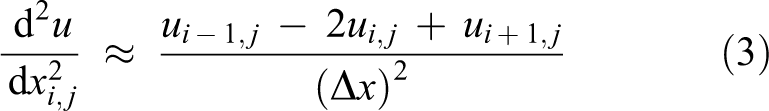
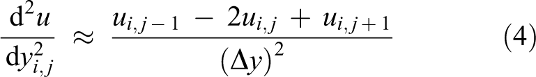
Putting the double partial derivatives in Laplace equation (2)

Since the pixels are spaced apart equally in both dimensions, we have Δx = Δy and equation (5) can further be rearranged as follows

Thus, we arrive at the discretized form of Laplace equation. From equation (6), it can be observed that the intensity of each pixel (i, j) in the hole region is governed by the intensity of pixels on the immediate left, right, top, and bottom. For every pixel in the hole area, equation (6) should be formed which results in the formation of multiple linear equations. These equations can then be solved using Gaussian or any other approach. The threshold for stopping could be calculated analytically or on the basis of the observations. Thus, the requisite region of the image shall be in-painted. The result of the explained method is shown in Figure 2(b).
Surface smoothing
After hole-filling, it is necessary to apply a smoothing filter as described in the beginning of “Hole filling and filter application” section to minimize the unwanted random fluctuations of pixels. Among the recently proposed filtering approaches presented by Milanfar, 26 we used the most well-known ones, bilateral filtering 27 and block matching 3-D (BM3D) filtering 28 approaches. In this section, we briefly review the theoretical concept behind these two filters.
Generally, there are two types of filters for image filtering: linear and nonlinear. Gaussian and averaging filters are the most well-known linear filters in spatial domain and perhaps the simplest way to smooth an image. In this method, each output image pixel value is a weighted sum of its surrounding pixels in the input image but since the value of neighbors is not considered, so in most cases, some kind of blurring occurs near boundaries. The action of such filters is independent of the image texture. The effect of each pixel on its neighbors depends only on its distance from each other, not on their actual values. In Gaussian filter, for example, the output image is given by the following equation
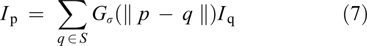
where I
p denotes the value of pixel
In bilateral filtering, the difference in value of surrounding pixels is taken into account to preserve edges while smoothing. In other words, two conditions should be satisfied for a pixel to influence another pixel in the output: It should occupy a nearby location and their value must be similar. The bilateral filter is defined by the following equation

where normalization factor Wp ensures pixel weights sum to 1.0

In equations (8) and (9), |.| denotes the absolute value. Bilateral filter is a nonlinear method in image filtering and is used in our experiments as a noise-reduction method. Although the criteria for comparing different noise reduction methods in most papers are almost signal-to-noise ratio, peak signal-to-noise ratio, or root-mean-square error, since the noise-free image is not accessible, in this article, we compare the effectiveness of our exploited noise-reduction techniques, in recognition rates, which will be discussed in the fourth section. Also it should be mentioned that the values of σs and σr in our experiments are considered to be 3 and 0.01, respectively. Further details about the implementation of bilateral filtering can be found in the study by Hernandez et al., 22 Milanfar, 26 and Tomasi and Manduchi. 27
The methods explained earlier are within the category of image filtering, which is called local approaches. Another attractive category in image denoising algorithms is nonlocal algorithms. In contrast to local approaches, in nonlocal algorithms, the output of filter in each pixel is not calculated anymore from the pixels that are closest to it, but from the pixels which have the most similar context, located anywhere in the image. BM3D belongs to this group of filtering approaches. 26,28 There are a number of researches applying the BM3D method for noise reduction in many applications like in synthetic-aperture radar image, 29 hyper-spectral imagery, 30 and so on. The results show the effectiveness of this method and motivated us to apply it in our experiment. BM3D algorithm is applied in two major steps: in the first step, the basic estimate is obtained through applying three steps into the noisy image, called grouping, collaborative hard thresholding, and aggregation. In the grouping step, original noisy image is searched for patches Q similar to the reference patch P. The similarity check is performed in the transform domain (commonly Hadamard–Walsh transform). A set of similar patches are stacked together to form a group. In order to speed up the process, we can keep only a predetermined number of patches that are closest to the reference patch in the 3-D group. Once the 3-D-block is built, the collaborative filtering is applied as follows: A 3-D discrete linear transform is applied followed by a shrinkage of the transform spectrum to remove noise components (collaborative filtering). Finally, temporary filtered blocks are obtained by applying the inverse of linear transform. Due to overlapping of patches, sometimes for a specific pixel, several estimates can be obtained. A particular averaging procedure called aggregation is exploited to eliminate this redundancy. The output of the first part of the algorithm is called basic estimate. In the second part, similar to the first part, block-matching takes place on a cleaner image as follows: Similar blocks of the basic estimate are found to form a 3-D matrix, for the 3-D matrix, 3-D transform is calculated using the Wiener filter, to obtain the final version of filtered patches, inverse 3-D filtering is performed and finally the obtained patches are aggregated to form the final estimate. It is observed in the experiments that the output of the second step improves the denoising performance while preserving more details especially near edges. More details about parameter selection of the BM3D algorithm can be found in the study by Lebrun. 31 We will further compare the results of applying the explained filtering approaches in our experiments in the fourth section.
Methodology of face detection, normalization, and recognition
Face detection and normalization
After hole filling and smoothing, the face area should be segmented from the whole image. Face detection can be done manually or using automatic methods. Since we decided to use algorithms using pointcloud for face detection, it is required to combine the RGB and depth images to form the pointcloud. By utilizing the colorful pointcloud for face detection, the segmented areas of both RGB and depth images will be obtained through mapping the pointcloud into the X-Y plane in two separate steps. First the RGB image is formed by mapping the color information of pointcloud and then the depth map can be formed in the same manner. We used the Kinect support package tool of MATLAB for making the pointcloud. The mentioned support package cannot form the pointcloud from the RGB and depth images if Kinect is disconnected from the PC. By connecting Kinect to the PC, mentioned support package can generate a colorful pointcloud, which means each point has the depth value as well as color information. The methods introduced by Hernandez et al., 22 Open, 32 and Malassiotis and Strintzis 33 apply pointcloud for face detection. We used the method proposed by Mian et al. 34 After segmenting the face, first the nose tip is detected because it has the lowest value in the depth map, as it is the nearest part of the body to the camera. More advanced methods can be used for detecting the nose tip. 34,35 Then, a sphere of radius r with its center located at the nose tip is used to crop the face area as well as its corresponding 2-D face. A constant value around 80 mm is found to be a good choice for radius of the sphere. It should be mentioned that in cases in which the nose tip is wrongly selected, the nose tip is elected manually and then the sphere is applied. After fitting the sphere and finding the face area, the RGB and depth image are extracted from the colorful pointcloud. Implementation of the mentioned method shows that the cropped region of both RGB and depth image of each pointcloud is exactly the same. RGB and depth images are normalized to 100 × 100 pixels and also all of RGB images are converted into gray level.
Feature extraction using curvelet transform
From one point of view, very similar to the categorization explained for image filtering, 3-D face recognition methods, which consider the effect of different facial expressions, can be divided into local and nonlocal approaches. Local approaches rely on the geometry of the face area. 3 They consider face as a 3-D surface and attempt to find different geometrical features of it to find the location or any especial property (like position, size, shape, volume, etc.) of some of the 59 common landmarks (a landmark is a point which is common in all faces and that has a particular biological meaning like eye, eyebrow, nose, and so on.) of human faces. These features are then used to search for other images with matching features. Vezzetti and Marcolin 36 used differential geometry of the face surface like coefficients of the fundamental forms and the derivatives and the shape and curvedness indexes to find the mentioned features. Most of these methods must be excluded the area under the nose, because it is not robust under different facial expressions. Recently, Ming 37 proposed a regional bounding spherical descriptor that can handle facial expressions with acceptable recognition rate. Although local approaches can handle partially occluded or posed faces better, they suffer mainly from two drawbacks: They are usually time-consuming, beside discrimination of surface geometry in noisy 3-D scans provided by Kinect is not easy even after noise reduction techniques, because these techniques may lessen the details by blurring some parts of image while local methods need the omitted details. In other words, they need high-resolution 3-D scans for getting promising results.
On the other hand, nonlocal approaches consider all visible facial information as a rigid object and focus on the global similarity of faces. Examples in this category include eigenface approaches such as our previous work 38 and multiresolution techniques such as wavelet transform. 7,39 Better recognition rates were achieved by applying these methods to face regions such as nose and eyes that are less sensitive to facial expression changes 40 but again finding these regions in a noisy depth map is not an easy task.
Multiresolution techniques have been applied successfully as a nonlocal approach in the field of face recognition. Wavelet is among the most well-known ones; however, 2-D-wavelet transform is an extension of its one-dimensional (1-D) and as all we know it has only three directions, namely, horizontal, vertical, and diagonal. So it is optimal only for point singularities and can reveal the image features across edges but not along edges. Human’s face includes a lot of curves and lines, and these features should be taken into consideration. There are a number of developments to form directional wavelet systems to analyze directional features of signals better. Some of them are contourlet, 41 shearlet, 42 and curvelet 43 transforms. They are uniformly called X-let transforms. Da costa et al. 44 applied the mentioned methods for 2-D face recognition and concluded that curvelet and shearlet transforms would perform much better than the other two methods. Thus, the revised version of curvelet transform 45 is selected to be used in our research.
Curvelet transform has been applied to many of 2-D and 3-D face recognition researches with successful results. 40,46 To the best of the authors’ knowledge, this work is the first one to investigate feature extraction using curvelet transform on 3-D face recognition using low-resolution Kinect images. To fulfill this task, we used both RGB and depth images of Kinect after preprocessing stage to extract features using curvelet transform.
Basically, continuous curvelet transform can be characterized by a couple of radial and angular windows in the frequency domain, W(r) and V(t), respectively. The argument of these windows is both nonnegative and real-valued and is supported on intervals r ∊ [1/2, 2] and t ∊ [−1, 1].
A polar wedge Uj can then be formed in the frequency domain on the basis of these two windows using the following equation

If Uj
is considered as the Fourier transform of a mother curvelet φj, then

Rθ is the rotation matrix by an angle θ. To discretize the continuous version of curvelet transform, Candes et al. 45 used two methods. The result is the following discrete curvelet coefficients
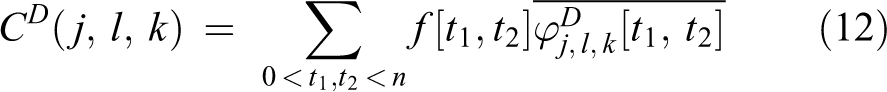
In which CD(j, l, k) are the curvelet coefficients and can be obtained using fast digital curvelet transform (FDCT). 45 There are two different digital implementations of FDCT, namely, unequally spaced fast Fourier transform and wrapping. As the second method is faster, it is used in our research.
FDCT via wrapping can be implemented as follows. 43
Let f[t
1, t
2] be the 2-D image and 2-D fast Fourier transform (2DFFT) of the image is taken, The product Wrap this product around the origin and obtain Apply the inverse 2DFFT to each
The number of scales can be obtained by the following formula 43

where m and n are the size of image. As our normalized size of images has 100 × 100 pixels, the scale will be 4, so there are four subbands for each image. Scales 1 and 4 represent subbands without angle decomposition. Scale 1 is called coarse level and is like a low-pass filter exhibiting the lowest frequency components of the image while scale 4 exhibits the highest frequency components revealing the edges of the image. We have also eight subbands at scale 2 (calling fine level) and 16 subbands at scale 3 (calling finest level).
Because in the frequency domain the coefficients at angle Θ and π + Θ are the same, only half of the subbands at fine and finest scales are used. As a result, the total number of subbands decreases to 4 at fine level and 8 at finest level. An example of a sample image in the database at gray level and depth level and their corresponding curvelet coefficients are shown in Figure 4. We extracted the curvelet coefficients for both RGB and depth images of all 30 persons in our database using the proposed method and used them in classification phase after dimension reduction.
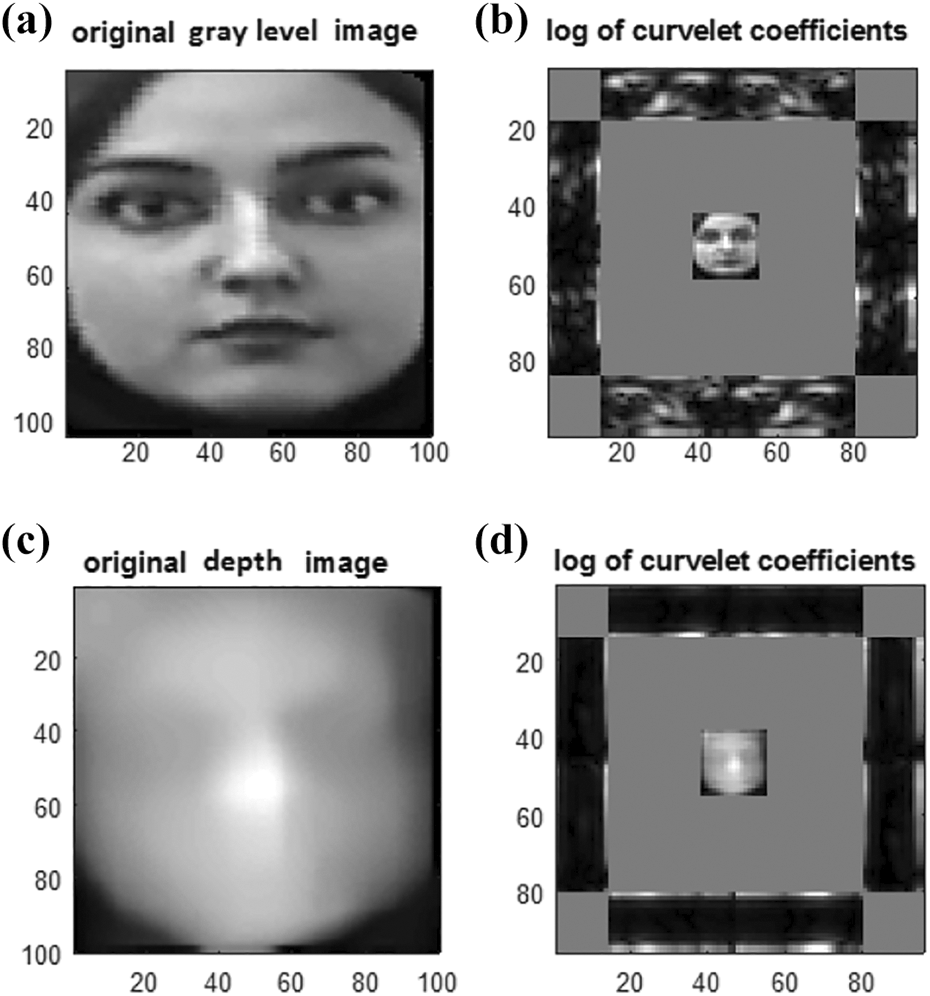
Original gray level of a sample image in the database (a), its corresponding curvelet coefficients (b), the depth map of the same image (c), and its corresponding curvelet transform (d).
Dimension reduction techniques
As stated in the previous section, according to formula (13), the scale for a 100 × 100 pixels image will be 4. Table 1 lists the amount of coefficients in each subband.
The amount of coefficients in each subband.

According to Table 1, the amount of curvelet coefficients is extremely large. So it is necessary to reduce the data feature vector using dimension reduction or feature selection techniques. Generally, dimension reduction techniques can be categorized into two main groups: supervised and unsupervised. In supervised learning—unlike the other method—the class labels is used for dimensionality reduction task, and as the class labels are given, it can be expected that just the features with related class should be selected. The basic concept behind all of supervised techniques can be summarized as follows: A good feature subset is one that contains features highly correlated with the specified class, yet uncorrelated with the features belong to every other classes. Linear discriminant analysis 47 and generalized discriminant analysis 48 are two well-known techniques that belong to this group of dimension reduction techniques. In unsupervised techniques, the algorithm must differ the relevant features from redundant features without knowing the class labels. Principal component analysis (PCA) and independent component analysis (ICA) belong to this category and are used in our experiments for dimension reduction. The details of their implementations can be found in the following two subsections.
Principal component analysis
A very popular method for dimension reduction is PCA.
49
It projects the data into a spatial domain and seeks the directions of highest variability. By computing the principal components of data and sorting it in decreasing order, the mentioned directions will be found. The first principal component corresponds to the direction of highest variability, the second corresponds for the next direction perpendicular to the first, and so on. It keeps the directions with the highest variability and excludes the rest and then maps the original data into a new lower dimension space. Considering the data matrix X consisting of 150 samples xi
(30 individuals each has 5 different expressions or occlusions) with D features (the values of D can be found from the amount of coefficients in Table 1, depending on the levels of subbands to be studied), the steps are as follows. 1. Computing the covariance matrix C

where
2. Computing the eigenvectors V and eigenvalues D using the covariance matrix obtained from the previous step as

3. After solving abovementioned equation, the eigenvector V should be sorted according to the values of its corresponding eigenvalue. The eigenvector with the highest eigenvalue is considered as principal component and shows the direction with the highest variability.
4. The last step is projecting the data matrix to the new space using the following equation

where Y is the projected data. The explained method should be applied to all four subbands of curvelet coefficients independently, and the projected data are used for classification.
Independent component analysis
While PCA tries to identify uncorrelated features from correlated ones and some of these uncorrelated features have most of information in the input attributes, the selected features of ICA analysis are both independent and uncorrelated. 50 Again by considering the data matrix X explained in the previous subsection, ICA assumes that the data matrix is linearly mixed with the source signals and tries to find the mixing matrix A

Equation (17) can be expressed as follows

In which the source signal is expressed in terms of mixed signals. It can be easily interpreted that W is inverse of A. We used fast ICA
51
for estimating W. After passing data centering and whitening steps, the following four steps will estimate W. 1. Choose an initial value for W. 2. Let

where

And g′(u) is the derivative of g. The g function can be replaced by any other nonlinear contrast function. Another possible choice is Gaussian function.
3. Normalizing W+ as follows

4. If W is not converged, that is, the value of W does not change over the next iteration, then go to step 2.
After finding W, its inverse A is computed and used as features for classification.
Classification using support vector machine
Support vector machine (SVM) used in our experiments is a well-known classifier. It is a highly nonlinear and single layer network with high ability to classify unseen data accurately. 52 It considers a separating hyperplane between the classes and tries to maximize the distance between the hyperplane and patterns. It uses an objective function based on the explained distances and the optimization process is carried out. A very popular and fast implementation of multiclass classification with SVM can be performed using LibSVM. 53 Different kernels are available for SVM in this package tool which can improve the performance of this classifier in some cases. Based on our experiments, the performance of the linear kernel is the best so we just report the results of using linear SVM.
Experimental results
To create a domestic database for face recognition in the presence of different facial expressions and occlusion, 30 individuals were selected. Each subject was captured under different combinations of four facial expressions, three poses, and one occlusion using sunglasses, resulting in a total of seven variations. The four expressions are neutral, happy, surprised, and angry. An occlusion was made using sunglasses. All of these expressions were taken with frontal pose. Two extra pictures were taken with neutral expression and 30° left and right profiles. The distance between the camera and the persons was between 900 mm and 1200 mm. Figure 5 shows a sample of the database with described facial expressions and poses.
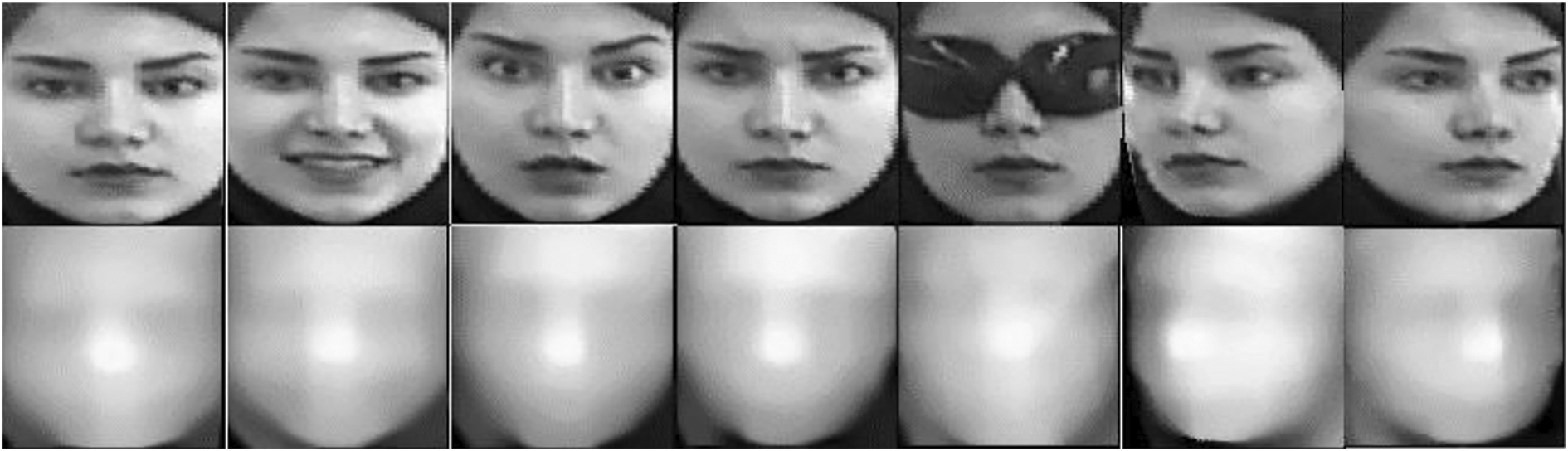
A sample image in the database with its different facial expressions and poses.
All experiments were carried out in MATLAB R2015b, on a 32-bit Quad CORE 3.6-GHz processor, with 4-GB RAM using our developed database. The database consists of images of 30 individuals each containing 4 different expressions and 1 occlusion, normalized to 100 × 100 pixels. These images include images obtained by converting the RGB images to gray-level images, and five depth images. We used four randomly selected images for training and one for testing. The recognition rates are shown in Figures 6 to 9 and Tables 2 to 7.

Rate of recognition using PCA, bilateral, and BM3D filtering of depth images for curvelet coefficients of four subbands with respect to the number of principal components (5, 8, 10…). PCA: principal component analysis; BM3D: block matching 3-D.

Rate of recognition using BM3D filtering of RGBD images for curvelet coefficients of four subbands. BM3D: block matching 3-D.

Comparison of recognition rates of depth, RGB, and RGBD images at coarse level.

Cumulative match characteristic curve on EURECOM database.
Rate of recognition without applying PCA.
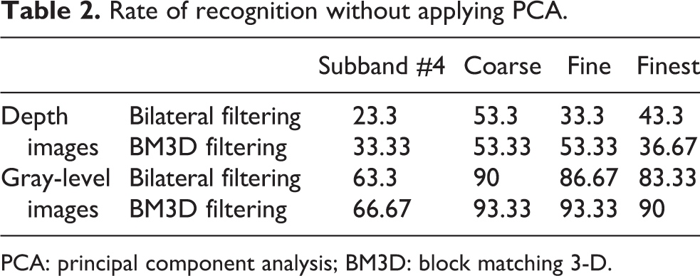
PCA: principal component analysis; BM3D: block matching 3-D.
Rate of recognition using PCA, bilateral and BM3D filtering of depth images.
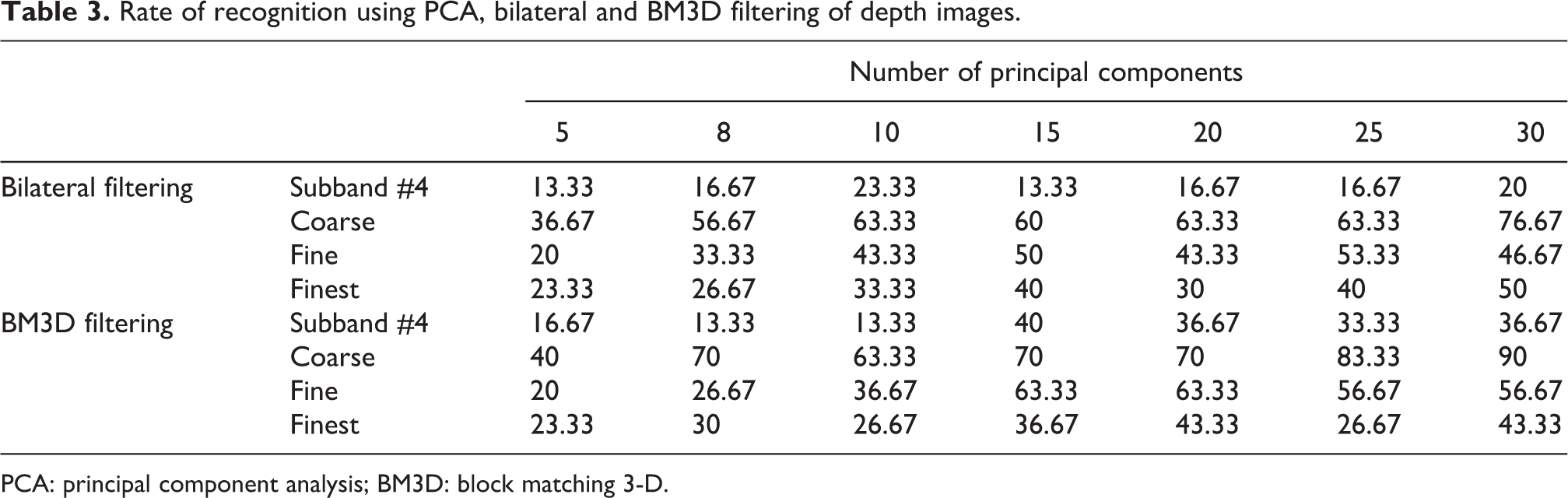
PCA: principal component analysis; BM3D: block matching 3-D.
Rate of recognition using PCA, bilateral and BM3D filtering of gray-level images.

PCA: principal component analysis; BM3D: block matching 3-D.
Rate of recognition using PCA and BM3D filtering of RGBD images.

PCA: principal component analysis; BM3D: block matching 3-D.
Comparing the recognition rates using PCA and ICA with different contrast functions.

PCA: principal component analysis; ICA: independent component analysis.
Comparing the recognition rates of RGBD images using PCA and ICA with different contrast functions.

PCA: principal component analysis; ICA: independent component analysis.
In the first experiment, we didn’t use dimension reduction techniques; the curvelet coefficients of each of four scales, namely, coarse, fine, the finest, and subband #4, were applied directly to SVM. It should be mentioned that the effects of applying bilateral and BM3D filtering were considered in all experiments.
Table 2 shows the recognition rates without applying dimension reduction. It can be seen that the recognition rates for depth images are absolutely disappointing and those are considerably higher when applying BM3D filtering instead of bilateral filtering. Also the first subband, that is, coarse coefficients of curvelet transform reaches the best rates and the fourth subband reaches the worst, both in gray-level and depth images.
Recognition rates are shown in Figure 6 and Table 3, after applying PCA with different number of principal components. As can be seen from Table 3, the rates of recognition for depth images are considerably higher than the rates without applying PCA. Again like the previously stated results, the rates of coarse level and BM3D filtering are higher than other subbands and filtering approach. The most important result is that we can achieve 90% recognition rate just using depth images when the number of principal components are 30 at coarse level of curvelet coefficients.
As expected, the recognition rates of gray-level images are higher than depth images; this is shown in Table 4. In Table 5, we show the recognition rates using RGBD images. It should be mentioned that just the outputs of BM3D filtering are within the table, as it outperforms the outputs of bilateral filtering. The RGBD images were created by concatenating the rows of the PCA output of both depth and gray-level data. We achieved 100% recognition rate when the principal component number of either of RGB or depth images was 25 or 30, respectively.
In Tables 6 and 7, the results of applying PCA and ICA are compared in terms of both recognition rate and consuming time. It should be mentioned that by applying the dimension reduction techniques several times, it was found experimentally that the optimal number for principal and independent components are 30 for PCA and 65 for ICA. By increasing the number of components, it was observed that the recognition rates decreased. As such, just the results of the mentioned optimal number of components are reported in Tables 6 and 7.
Another important result derived from Tables 3 to 5 is that although the best recognition rate belongs to curvelet coefficients at coarse level, but coefficients at the fine and finest levels also led to good results, revealing the proper power of curvelet transform in angular decomposition.
From Tables 6 and 7, it could be derived that the processing time of dimension reduction using ICA is considerably higher than PCA; however, the recognition rates are not much higher. Since the result of ICA will change in each iteration, the reported result is the average value obtained by 5 times application of ICA.
In the last three figures, some aspects of the tables are depicted for comparing the results better. Figure 7 shows that the best level of curvelet coefficients belongs to coarse level, also fine level coefficients have acceptable results. Figure 8 shows the recognition rate of BM3D filtering at coarse level when using each of depth or RGB images alone and when the combination of them used as feature space. These results clearly show that combining the RGB and depth images is better than using the depth or RGB images alone.
We also applied our proposed algorithm on EURECOM 54 —a publicly available data set. It consists of 53 individuals each having 18 images captured in 2 different sessions and under different poses, illuminations, and facial expressions and also occlusions. Each image also has a text file containing position of six landmarks of every face. The third landmark is the position of nose tip which is used in our experiment as the center of image and all of the images were normalized to 100 × 100 pixels by considering the nose tip as the center of image at position (50, 50). We also discarded the left and right profile of subjects in either sessions. Table 8 shows the results of applying our proposed algorithm on EURECOM database. It should be mentioned that PCA is used for dimension reduction and the number of principal component assumed to be 30. It should be noted that according to the results of Table 8, coefficients of the finest level alone reached 92.6% which is very close to the highest identification rate at the coarse level. Also, the corresponding cumulative match characteristic curve is shown in Figure 9.
Identification rates of the proposed algorithm on EURECOM database.

Table 9 compares the results of previous works using EURECOM database with our proposed algorithm. As can be seen clearly, our method outperforms others both in using depth images alone and when using RGB and depth images simultaneously.
Comparison of the recognition rates of previous researches with different denoising and feature extraction approaches.

BM3D: block matching 3-D; SIFT: scale-invariant feature transform; HOG: histogram of oriented gradients; COV: covariance descriptor; LBP: local binary pattern; SURF: speeded up robust features.
Conclusion and future work
This article presents an approach for face recognition using Kinect. The proposed method is able to overcome challenges like nonmeasured pixels and noisy pixels in a low-cost 3-D scanner such as Kinect. Experimental results show that the proposed method can reach 100% recognition rate on the domestically developed database. This database is available for further academic research.
This work aimed to account for the impact of different facial expressions and occlusions, and we excluded the left and right profiles in our experiments. The mentioned profiles will be included in our near future research.
Key findings of this work can be outlined as follows. For image smoothing, two recently proposed filtering approaches, that is, bilateral filtering as a representative for local approaches and BM3D filtering as a representative for nonlocal approaches, were used. As shown in experimental results, BM3D filtering provides higher recognition rate than bilateral filtering. The whole process of creating a domestic database for 3-D face recognition is explained using just a simple Kinect sensor and a laptop. The whole process is accomplished with MATLAB software, without requiring any auxiliary software or hardware. Although 1-D wavelet transform used in many applications with outstanding results, its extended 2-D form has limitation to extract the features along curves. On the other hand, face recognition under different facial expressions is highly dependent on the line and curves of the captured face; therefore, another kind of multi-scale representation tool, curvelet transform, is chosen to extract facial expression feature, which is proved to be effective in experiments. Also the effectiveness of all output subbands of this nonlocal feature extraction approach was evaluated in the classification stage. Conclusion is that the features of coarse and fine levels have more discriminant power, to be used for classification, than the two other subbands. Since the number of features extracted by curvelet transform is very high, dimension reduction techniques must be applied to feature space. As shown in our experiments, the reduced features considerably outperform the whole feature space especially in depth images. Also we compared two well-known unsupervised dimension reduction techniques, namely, PCA and ICA, and surprisingly observed that the results of PCA method outperform ICA in terms of processing time and recognition accuracy. Combining depth and RGB images, as expected, can improve recognition rates significantly.
Footnotes
Declaration of conflicting interests
The author(s) declared no potential conflicts of interest with respect to the research, authorship, and/or publication of this article.
Funding
The author(s) received no financial support for the research, authorship, and/or publication of this article.