Sage Journals: Discover world-class research

Abstract

A multi-robot system consists of a number of autonomous robots moving within an environment to achieve a common goal. Each robot decides to move based on information obtained from various sensors and gathered data received through communicating with other robots. In order to prove the system satisfies certain properties, one can provide an analytical proof or use a verification method. This article presents a new notion to prove visibility-related properties of a multi-robot system by introducing an automated verification method. Precisely, we propose a method to automatically generate a discrete state space of a given multi-robot system and verify the correctness of the desired properties by means of model-checking tools and algorithms. We construct the state space of a number of robots, each moves freely inside a bounded polygonal area with obstacles. The generated state space is then used to verify visibility properties (e.g. if the communication graph of robots is connected) by means of the construction and analysis of distributed processes model checker. Using our method, there is no need to analytically prove that the properties are preserved with every change in the motion strategy of the robots. We have implemented a tool to automatically generate the state space and verified some properties to demonstrate the applicability of our method in various environments.

Keywords

Formal methods for robotics distributed robotics systems verification

Introduction

In multi-robot systems (MRS), a collection of two or more autonomous robots can solve problems in a broad range of applications by collaborating with each other and sensing environments. For example, teams of mobile robots have been used for inspection of nuclear power plants,¹ aerial surveillance,² search and rescue,³ and underwater or space exploration.⁴ In many applications within the general area of robot motion planning, visibility problems play an important role.

There has been a close relationship between robot motion planning and computational geometry in the applications where the robots navigate within a geometric domain. Traditionally, there has been a research area with the goal of minimizing the number of (stationary) guards or surveillance cameras to guard an area in the shape of a certain geometric domain like extensions of art gallery problems.⁵ Moving to the area of mobile guards, Durocher et al.⁶ considered the sliding cameras problem in which the cameras travel back and forth along axis-aligned line segments inside an orthogonal polygon. In the Minimum Sliding Cameras (MSC) problem, the objective is to guard the polygon with the minimum number of sliding cameras. In MSC problem, it is assumed that the polygon is covered by the cameras if the union of the visibility polygons of the axis-aligned segments equals the polygon. One of the original works on the subject of mobile guards is studied by Efrat et al.,⁷ considering the problem of sweeping polygons with a chain of guards. They developed an algorithm to compute the minimum number of guards needed to sweep a polygon.

Commonly, within the context of computational geometry such as the previous works mentioned above, analytical proofs are provided to show that the given robot navigation algorithms satisfy some certain properties (e.g. global connectivity among the robots is always preserved). In cases when the planning algorithms get complex, it may be hard or even impossible to provide any analytical proofs. Furthermore, when it comes to practical applications of robot navigation algorithms, in order to find a solution that satisfies the problem’s constraints, the designer may adjust some algorithm’s parameters or refine the algorithm in such a way that the whole robot movement strategy changes. This way, it may not be practical to repeatedly provide analytical proof for such modified algorithms.

An alternate and more reliable approach to investigate the correctness of the motion algorithms is formal verification, specifically, model-checking,⁸ which has become more popular in recent years. Here, a mathematical model of all possible behaviors of the system is constructed, often as a state transition system, and is automatically verified against the desired correctness properties over all possible paths. The properties are often expressed in temporal logic formulas.

In some previous works, model-checking has been used to verify motion planning algorithms with respect to problem’s constraints. In Fainekos et al.,⁹ the authors used a discrete representation of the continuous space of the movement of a single robot, producing a finite state transition system. Later, Fainekos et al.¹⁰ extended the previous framework to multiple robots. These frameworks generate a motion plan for the robot to meet some regions of interest inside a polygon in order to satisfy a given linear temporal logic (LTL)¹¹ formula.

Another related area to which model-checking techniques have been applied are robot swarms. In Liu and Winfield,¹² a swarm of foraging robots is presented and, in Konur et al.,¹³ is analyzed using the probabilistic symbolic model checker.¹⁴ A hierarchical framework for model-checking of planning and controlling robot swarms is suggested by Kloetzer and Belta¹⁵ to make some abstraction of the problem including the location of the individual robots. Dixon et al.¹⁶ used model-checking techniques to check whether desired temporal properties are satisfied to analyze emergent behaviors of robotic swarms. Moreover, Brambilla et al.¹⁷ introduced property-driven design, a top-down design method for robot swarms based on prescriptive modeling and model-checking. In 2014, Guo and Dimarogonas¹⁸ proposed a knowledge transfer scheme for cooperative motion planning of multi-agent systems. They assumed that the workspace is partially known by the agents where the agents have independently assigned local tasks, specified as LTL formulas.

More recently, Sheshkalani et al.^19,20 focused on the verification of certain properties on an MRS in a continuous environment. In Sheshkalani et al.,¹⁹ the robots were assumed to move along the boundaries of a given polygon. They constructed a transition system on which the visibility properties can be investigated. Later, Sheshkalani et al.²⁰ made the problem more general and let the robots move along simple paths inside the environment.

We believe that the results presented by Sheshkalani et al.^19,20 are restrictive in the sense that the robots are only allowed to move along predefined paths within a simple polygon. So, in this work, we propose a method to overcome the previous restrictions. Specifically, this article is different from the previous work²⁰ in the following points:

A new notion of state definition is proposed, so that robots can navigate the environment freely without any movement restrictions.

It is allowed to have obstacles inside the environment.

A theoretical discussion is provided to show that the number of states is finite.

To demonstrate the applicability of the proposed method, some simulation results are provided in various environments over two case studies (e.g. a decentralized swarm aggregation algorithm²¹).

As an application of the problem studied in this article, the problem of guarding a bounded environment with a number of sliding cameras can be viewed as a special case of our problem. This way, our method is related to the previous study.⁶ Note that the mentioned study address the combinatorial optimization problem of minimizing the number of cameras. On the other hand, we address the problem of verifying the correctness of the motion strategies for the given system. Another, more interesting, application of the problem is to consider the connectivity preserving (global connectivity maintenance) of the communication graph. Sabattini et al.²² proposed a method to preserve the strong connectivity by estimating the algebraic connectivity of the communication graph in a decentralized manner. This way, our method can be used to guarantee the correctness of the desired requirements related to the Connectivity property.

The inputs to our method are comprised of (1) the environment, in the form of a polygon with obstacles, (2) the algorithms controlling the motions of the robots, (3) the initial positions of robots, and (4) the correctness property, expressed as a temporal logic formula. The output of the method is a True/False answer to the desired property as well as a transition system, labeled by two visibility-related atomic proposition: Connectivity (the communication graph of the robots is connected) and Coverage (the robots can collectively see the entire environment). The generated transition system is used to model check the visibility properties expressed in temporal logic formulas over the mentioned atomic propositions. The problem is defined more elaborately in the “Preliminaries and problem definition” section.

Our method is abstract from the specific motion planning algorithms in the sense that each robot may be programmed with a separate algorithm which during the execution may cause the robot to sense the surroundings through various sensors or perform communications with other robots. Precisely, the robots’ navigation algorithms are seen as a black box which means that the required information (e.g. other visible robots’ locations and the geometry of the their surroundings) are given to each algorithm as the inputs, and then the output of the algorithms provides a decision about the next movement of the robots (e.g. in the form of a pair of values for the direction and the distance). In the end, all the sensing, communication, and internal logic lead to movement steps which are treated as actions by our method, causing transitions between states.

In general, the environments in which the robots navigate can be discrete (e.g. a grid) or continuous. In the discrete environments,¹⁶ a state is a snapshot of the grid which specifies the cells that have some robots inside (static discretization). In contrast to the discrete environments, when talking about continuous domains (like this work), the robots may move continuously to any arbitrary locations inside the environment. So, we need to dynamically discretize the environment in such a way that the underlying properties can be verified. This way, we define a notion of state for such a system to construct a transition system on which the properties can be verified using the conventional model-checking algorithms (“Constructing the discrete state space” section).

Additionally, we provide a proof of correctness for the proposed state space generation algorithm and show that the size of the state space is bounded (“Analysis” section). Finally, to give some intuition about the number of states and the amount of time needed to be generated, we have implemented a tool to automatically generate the state space and verify the correctness of some requirements using the construction and analysis of distributed processes (CADP)²³ tool to demonstrate the applicability of our method in two case studies explained in “Case studies” section.

Preliminaries and problem definition

The following definitions are borrowed from Ghosh.²⁴ A polygon P is defined as a closed region in the plane bounded by a finite set of line segments (called edges of P) such that there exists a path between any two points inside P that intersects no edge of P. Each endpoint of an edge of P is called a vertex of P. A vertex of P is called convex if the interior angle at the vertex formed by two edges of that vertex is at most 180°; otherwise it is called reflex.

Definition 1

Visibility.²⁴ Two points r_i and r_j in P are said to be visible if the line segment joining r_i and r_j contains no point on the exterior of P. This means that the segment $\bar{r_{i} r_{j}}$ lies totally inside P. This definition allows the segment $\bar{r_{i} r_{j}}$ to pass through a reflex vertex or graze along a polygonal edge. We also say that r_i sees r_j if r_i and r_j are visible in P. It is obvious that if r_i sees r_j, r_j also sees r_i.

For a polygon P with obstacles, we use the notation $V_{r_{i}}$ for the visibility polygon of a point r_i ∈ P. Removing $V_{r_{i}}$ from P may result in a number of disconnected regions called invisible regions. Any invisible region has exactly one edge in common with $V_{r_{i}}$ , called a window of r_i, which is characterized by a reflex vertex of P visible from r_i, like q. The window is defined as the extension of the (directed) segment $\bar{r_{i} q}$ from r_i to the boundary of P, say x_j. We denote such a window which consists of two endpoints q and x_j by $r_{i} q^{\to}$ . As depicted in Figure 1, the windows of r₃ consist of $r_{3} p_{3}^{\to}$ , $r_{3} o_{1}^{\to}$ , $r_{3} o_{3}^{\to}$ , and $r_{3} p_{8}^{\to}$ .

Figure 1.
The shaded area indicates the visibility polygon of point r₃ ( $V_{r_{3}}$ ). Point r₁ is invisible from r₃, and its containing invisible regions are characterized by the reflex vertices p₃, p₈, o₁, and o₃ which are separated from $V_{r_{3}}$ by line segments $\bar{p_{3} x_{1}}$ , $\bar{p_{8} x_{2}}$ , $\bar{o_{1} x_{4}}$ , and $\bar{o_{3} x_{3}}$ as well.

Consider a polygon P with obstacles whose boundary is specified by the sequence of n vertices $〈 p_{1}, p_{2}, \dots, p_{n} 〉$ , the boundary of obstacles $O = {o_{1}, o_{2}, \dots, o_{m}}$ with m vertices, including the set of reflex vertices Reflex and convex vertices Convex, a set of robots $R = {r_{1}, r_{2}, \dots, r_{k}}$ , and the corresponding navigation algorithms $A l g = {a_{1}, a_{2}, \dots, a_{k}}$ (a_i is the navigation algorithm of robot r_i) are given with the following properties:
Each robot r_i acts based on the corresponding navigation algorithm a_i inside P.

Each step in the movement of each robot is specified by a pair (θ, δ) where θ is the direction of the movement, and δ is the distance the robot moves (both values are real positive numbers).

To study the characteristics of the system, we use state space which is a mathematical model of a physical system. Each state is connected to some related states by means of transitions. To discretize the state space of the system, we assume that the robots have turn taking movements (e.g. during the movement of a robot, the position of other robots is fixed), as described by Dixon et al.¹⁶ and Antuña et al.²⁵ As stated in Peled et al.,²⁶ it is possible to have one of the following cases in order to check automatically the properties of a finite state system whose structure is unknown: (a) a precise bound l on the number of states is known, (b) the size of the state space is not known precisely: an upper bound l is available, and (c) no bound l is known on the number of states. Since our method is abstract from the specific motion planning algorithms (each algorithm in Alg set is treated as a black box), no bound l is available on the number of states. So, as Peled et al.²⁶ suggested for case (c), we may let our method run so long as the available time and space resources allow. This way, the guarantees depend on the running time of our proposed method. Since the robots usually have a specific common goal which prevents the robots from making arbitrary actions, the number of generated states converges (no new state is generated after a significant amount of time running the proposed method) reasonably fast as is shown in “Case studies” section.

The correctness properties may be described using temporal logics which are formalisms to express temporal properties of reactive systems.²⁷ Apart from the logical operators, temporal logic formulas are constructed over a set of atomic propositions which may be True or False in each state of the system. To the discussion in the previous paragraph, since it is not possible to be sure that the constructed state space is complete, we have to evaluate LTL over finite traces, namely LTL_f.²⁸ As stated by De Giacomo et al.,²⁹ LTL_f uses the same syntax as of the original LTL.¹¹ The classical LTL formulas have different meanings on finite traces as discussed by De Giacomo and Vardi.²⁸ To bring an example, the following are some classical LTL formulas and their meaning on finite traces:
“Safety”: □φ means that always till the end of the trace φ holds.

“Liveness”: ⋄φ means that eventually before the end of the trace φ holds.

We refer the reader to previous studies^28
–30 for related discussion about LTL over infinite and finite traces. From now on, the LTL modalities □ and ⋄ are interpreted according to LTL_f semantics.

Since our goal is to verify visibility properties, we need to define the two following properties:

Definition 2

Connectivity. The set of robots are connected if the graph induced by the visibility relation between pairs of robots is connected.

Definition 3

Coverage. The robots cover P if the union of the visibility polygons of all robots $(\underset{r_{i} \in R}{\cup} V_{r_{i}})$ covers the whole P.

Since we do not deal with the details of model-checking algorithms directly in this article, we refer the reader for a detailed description of temporal logics to Baier and Katoen.²⁷ However, to bring an example, the LTL_f formula $□ ((C o n n e c t i v i t y \land \neg C o v e r a g e) \to ⋄ (C o n n e c t i v i t y \land C o v e r a g e))$ describes the property that whenever the visibility graph of robots is connected but the environment is not covered, eventually the system reaches a state in which both Connectivity and Coverage properties are satisfied (robots will eventually cover the environment by collaborating with each other).

We define an MRS as the tuple $(P, O, R, A l g, i n i t)$ in which P indicates the environment, O defines the boundary of obstacles inside P, R is the set of moving robots, Alg is the set of navigation algorithms of robots, and init specifies the initial position of robots inside P. The navigation algorithms used for robots model are assumed to be deterministic. Our goal is to define the transition system corresponding to MRS, over which temporal logic formulas can be model checked. The states of this transition system are abstractions of the robots’ configuration, and the transitions among the states occur as the robots move inside the environment.

Constructing the discrete state space

With the ultimate goal of verifying a temporal logic formula over an $MRS = (P, O, R, A l g, i n i t)$ , we must first construct the corresponding transition system of MRS. As mentioned before, the states are labeled with the atomic propositions, hence, the transition system is called a labeled transition system (LTS).^31,27

We define the LTS of MRS as the tuple $(S, A c t, ↪, s_{0}, A P, L)$ where
S is the set of states (defined below);

Act is the set of actions denoting the movements of the robots (precisely defined in subsection Transition Events);

$↪ \subseteq S \times A c t \times S$ is the transition relation, (we use the notation $s \overset{α_{j}}{↪} s^{'}$ whenever $(s, α_{j}, s^{'}) \in ↪$ );

$s_{0} \in S$ is the initial state (determined based on init);

$A P = {C o n n e c t i v i t y, C o v e r a g e}$ is the set of atomic propositions; and

$L : S \to 2^{A P}$ is the labeling function.

System states

The satisfaction of AP depends on the distribution of the robots’ position inside P. We model each state of the system based on the topology of the robots and the vertices of P.

Consider the union of all the windows of the robots $W = {r_{i} q^{\to} | r_{i} \in R, q \in R e f l e x \cap V_{r_{i}}}$ . The intersection of the line segments in W results in a subdivision inside P which is denoted by Sub_P (Figure 2). The subdivision Sub_P is comprised of a number of cells denoted by c_i for 1 ≤ i ≤ 10 in which each cell is bounded by some windows and polygonal edges (e.g. cell c₃ is bounded by the line segments $r_{3} o_{1}^{\to}$ , $\bar{p_{1} p_{10}}$ , $r_{3} o_{3}^{\to}$ , and $\bar{o_{3} o_{1}}$ ). The obtained subdivision has some useful visibility-related characteristics. Precisely, the number of visible robots in each pair of cells that has an edge in common but different in one.²⁴ In other words, the number of robots which are visible in the entire cell is the same. This way, we can dynamically abstract out the precise location of the robot inside the cell. Since we need to deal with the overall structure of the subdivision (proximity of the cells) and not the precise positions of the intersection points, we use the corresponding dual graph of the subdivision (Definition 4).

Figure 2.
A subdivision which consists of the intersection of line segments in W inside P.

Definition 4

Dual graph. Let Sub_P be a subdivision of P. The dual graph of Sub_P that is represented by $D G (S u b_{P})$ is a graph which has a node corresponding to each cell, and each pair of nodes is connected with an edge, iff their related cells have an edge in common.²⁴

Consider Figure 2. Based on the Definition 4, we assign a node (denoted by n_i for 1 ≤ i ≤ 10) corresponding to each cell of the subdivision (Figure 3). Next, we connect each pair of nodes with an edge, iff their related cells have an edge in common. The obtained $D G (S u b_{P})$ is depicted in Figure 4. Furthermore, we label each node of $D G (S u b_{P})$ with the set of the windows and the polygonal edges which determine the boundary of the corresponding cell in Sub_P. As an example, consider the cell c₁ of Sub_P as depicted in Figure 2. This cell is bounded by the line segments $r_{1} o_{1}^{\to}$ , $r_{2} p_{9}^{\to}$ , and $r_{3} p_{3}^{\to}$ . The corresponding node of cell c₁ in $D G (S u b_{P})$ is n₁. So, we label node n₁ with the set ${r_{1} o_{1}^{\to}, r_{2} p_{9}^{\to}, r_{3} p_{3}^{\to}}$ .

Figure 3.
The corresponding node of each subdivision’s cell is depicted (denoted by n_i).

Figure 4.
The dual graph of subdivision Sub_P.

The dual graph $D G (S u b_{P})$ does not change unless some cells are removed from or added to Sub_P. Therefore, we may use the dual graph of P to represent Sub_P. Since the satisfaction of AP can be determined by analyzing Sub_P (Lemma 1), we can store $D G (S u b_{P})$ as a part of each state.

Assume that we consider $D G (S u b_{P})$ as the definition of the states. To build the state space, we have to compute the successors of each state, determined by the movements of the robots. Precisely, if $D G (S u b_{P})$ is considered as the definition of the states, since the structure of the subdivision depends on the location of the robots, the next changes to the subdivision completely depend on the direction and the distance values (θ, δ) each robot’s navigation algorithm calculates for the next movement. Hence, we need to keep track of the changes to $D G (S u b_{P})$ as the robots move. Suppose robot r_i moves in a certain direction θ. The set of windows of r_i $(W_{r_{i}} = {r_{i} q^{\to} | r_{i} \in R, q \in R e f l e x \cap V_{r_{i}}})$ may move radially around p_i s during the movement of r_i respectively. During the movement of the line segments in $W_{r_{i}}$ , new cells may be constructed in Sub_P or existing ones may be destructed. Construction or destruction of cells may happen if and only if some line segment in $W_{r_{i}}$ intersects some vertex of Sub_P.

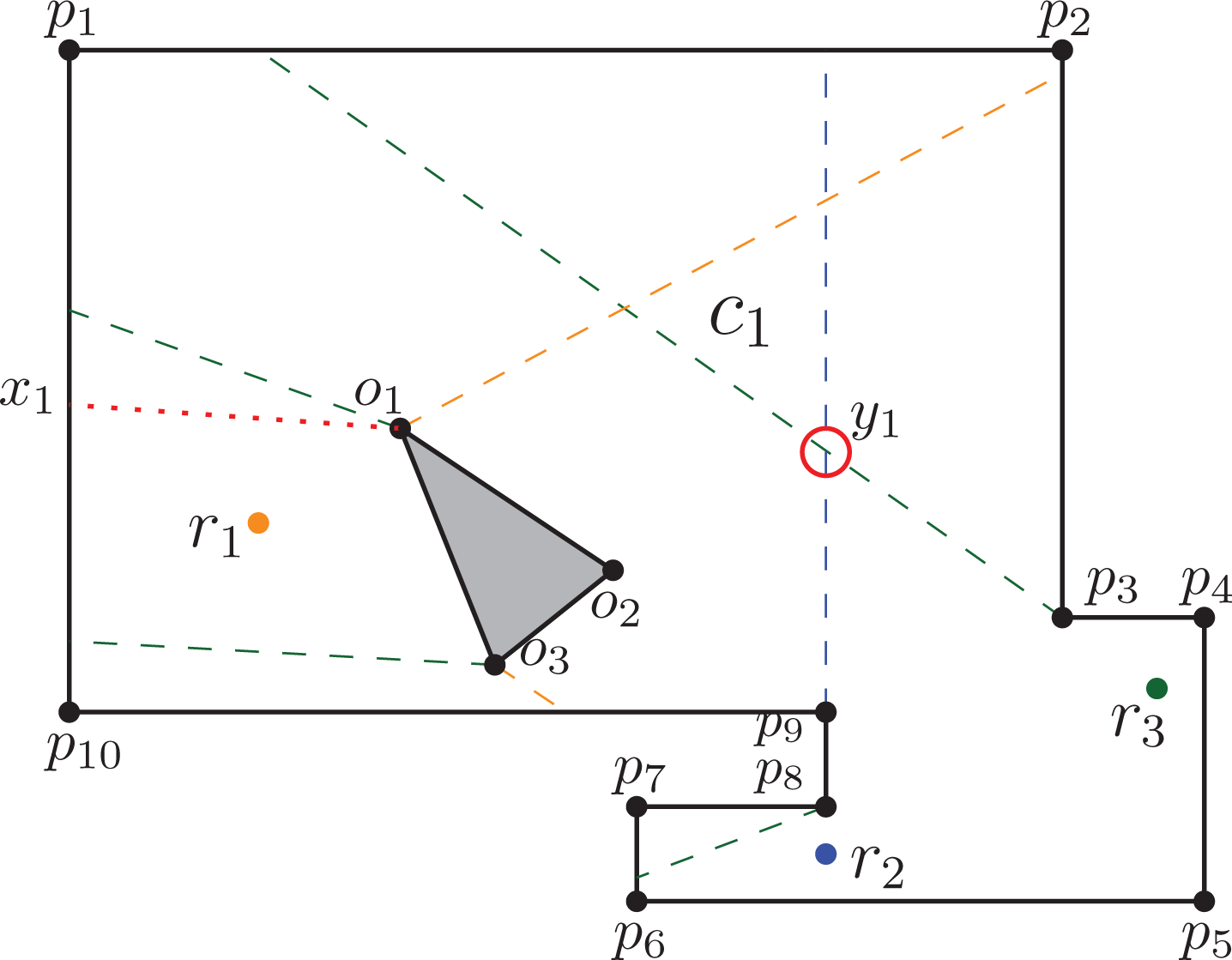
As an example, consider Sub_P as depicted in Figure 5. Suppose that r₁ decides to move toward p₁ (while other robots stand still). Consequently, the window $r_{1} o_{1}^{\to}$ rotates in the clockwise direction. As the movement continues, eventually cell c₁ disappears (Figure 6). It is easy to see that this happens when r₁ crosses the dotted line segment $\bar{o_{1} x_{1}}$ . The line segment $\bar{o_{1} x_{1}}$ belongs to $y_{1} o_{1}^{\to}$ , where y₁ is the intersection point of $r_{2} p_{9}^{\to}$ and $r_{3} p_{3}^{\to}$ . Using the encoding of $D G (S u b_{P})$ expressed in the Definition 4, we cannot determine such transitions. So, to be able to compute the successor states correctly, we have to include more information in the states. So, we need to store the windows of the intersection points of Sub_p (e.g. y₁) besides $D G (S u b_{P})$ as a definition of the states (Definition 5) in order to determine the successor states.

Figure 5.
Connectivity and Coverage properties are not satisfied.

Figure 6.
Robot r₁ moves toward p₁ in such a way that it crosses $y_{1} o_{1}^{\to}$ . The Coverage property is then satisfied.

Let $N (S u b_{P})$ denotes the vertices of the subdivision Sub_P. Consider the union of all the windows of $N (S u b_{P})$ , namely $W^{'} = {p q^{\to} | p \in N (S u b_{P}), q \in R e f l e x \cap V_{p}}$ . The intersection of the line segments in W′ results in another subdivision $S u b_{S u b_{P}}$ . This way, we obtain a more fine-grained subdivision by overlaying Sub_P and $S u b_{S u b_{P}}$ , which is denoted by $S u {b^{'}}_{P}$ (Figure 7). So, a robot may change $D G (S u b_{P})$ (destruct or construct a new cell) if and only if it crosses one of the line segments of $S u b_{S u b_{P}}$ . For example, line segment $\bar{o_{1} x_{1}}$ belongs to the subdivision $S u {b^{'}}_{P}$ as shown in Figure 6. Storing $D G (S u {b^{'}}_{P})$ as a part of each state (Definition 5) is necessary and sufficient to compute the successor states regarding the transition types described in the next section (Lemma 2).

Figure 7.
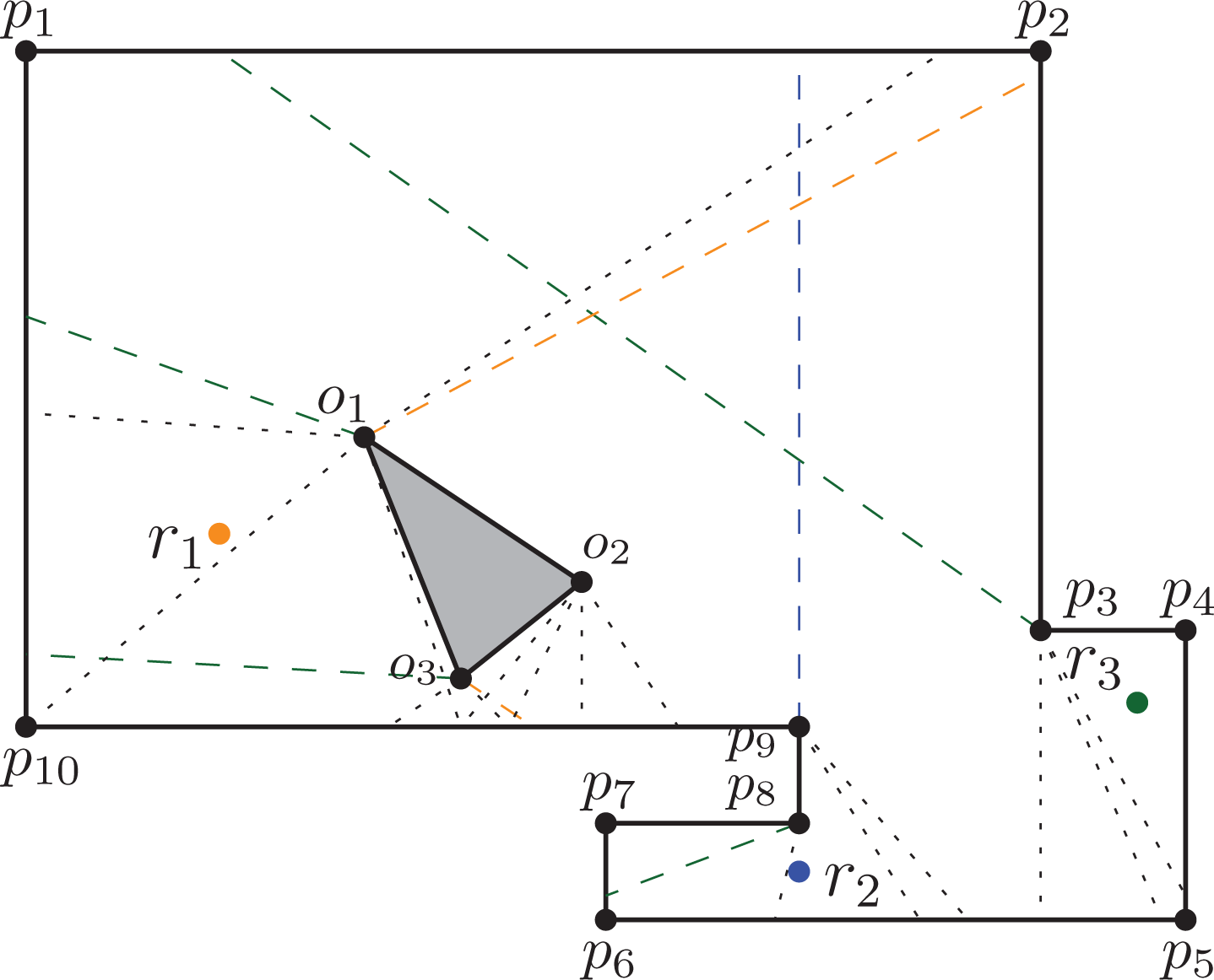
Overlaid subdivisions of Sub_P (dashed line segments) and $S u b_{S u b_{P}}$ (dotted line segments) which results in $S u {b^{'}}_{P}$ .

Definition 5

State. We define a state of k robots inside the polygon P as the pair:
$D G (S u b_{P})$ along with the robots in each cell of Sub_P, and

$D G (S u {b^{'}}_{P})$ along with the robots in each cell of $S u {b^{'}}_{P}$ .

To conform the standard notion of LTS, we must show that each atomic proposition is either True or False in a state. The following lemma states that moving of the robots does not change the validity of the propositions Connectivity and Coverage, as long as the state defined above remains the same.

Lemma 1

Each state s can be uniquely labeled with the atomic propositions $A P = {C o n n e c t i v i t y, C o v e r a g e}$ .

Proof outline

Assume that the labeling $L (s) \in 2^{A P}$ is satisfied by the current state s. It is sufficient to prove that by moving the robots, L(s) is valid as long as the configuration of the robots yields in the same state s. We discuss the two atomic propositions separately.

Connectivity

Two robots r_i and r_j are connected, if one lies in the visible area of the other $(r_{i} \in V_{r_{j}})$ . Since the boundary of the visible area for each robot is determined by its corresponding windows $(W_{r_{j}})$ that are stored as the line segments in Sub_P, we can decide whether robot r_i is located inside $V_{r_{j}}$ . Assume that robots r_i and r_j are connected, and they are located in cells c_i and c_j, respectively (based on Sub_P). If r_i moves to get disconnected, it must cross one of the line segments in $W_{r_{j}}$ . In this case, r_j does not belong to c_j anymore. So, the current state s changes based on the definition of state.

Coverage

Polygon P is covered if and only if all the cells in Sub_P are covered by the robots. Assume that there exists at least one cell, say c₁, which is not visible from any of the k robots (Figure 5). The polygon remains uncovered as long as c₁ is not destructed. More precisely, the polygon may become covered if the uncovered cells destructed. On the other side, assume that all the cells of Sub_P are covered by the robots. In order to make P uncovered, a new cell which is not visible from the robots to be constructed in Sub_P is needed. Since any changes in validity of Coverage need to make Sub_P different from its previous structure, Coverage is valid while s does not change. □

Transitions events

During the execution of an MRS, when the robot r_i takes its turn to move, its motion algorithm a_i determines the next step of the movement as a pair (θ, δ), where θ is the direction of the movement and δ is the distance the robot moves. Based on the position of r_i, it may cross one of the boundary edges of the cell it currently resides in. So, the movement with distance δ may result in a sequence $〈 α_{1}, α_{2}, \dots, α_{m} 〉$ , where $α_{j} \in R \times {W \cup W^{'}}$ denotes that r_i has crossed one of the windows in ${W \cup W^{'}}$ . We define the actions of the transition system $A c t = R \times {W \cup W^{'}}$ as the set of all possible crossing events as mentioned above.

We define the transition relation of the LTS, say ↪, as the smallest relation containing the tuples $(s, α_{j}, s^{'})$ , where $s, s^{'} \in S$ , and s′ is the state obtained from robot r_i crossing a window $r_{i} p_{j}^{\to}$ , where $r_{i} p_{j}^{\to}$ is any window bounding the cell containing r_i. While r_i is making its movement, a transition $s \overset{α_{j}}{↪} s^{'}$ can occur in the following transition types:
Some cells constructed or destructed in Sub_P which leads to changes in $D G (S u b_{P})$ .

A robot crosses a window of W and moves into another cell of Sub_P.

If none of the two above types have occurred after the movement of the robot, it must be checked whether $D G (S u {b^{'}}_{P})$ has changed. If that is the case, we need to have a transition to s′ with the same $D G (S u b_{P})$ as of s but having $D G (S u {b^{'}}_{P})$ updated.

As an example, consider Figure 5 (both Connectivity and Coverage properties are not satisfied). Assume that robot r₁ moves toward p₁. As depicted in Figure 6, it destructs cell c₁ and makes Coverage property satisfied (transition type (a)). Furthermore, based on Figure 8, robot r₁ moves again toward p₁ till reaches window $r_{3} o_{1}^{\to}$ (transition type (b)). This way, robots r₁ and r₃ become visible to each other which satisfies the Connectivity property as well.

Figure 8.
Connectivity property is satisfied after r₁ crosses $r_{3} o_{1}^{\to}$ while moving toward p₁.

We may use the plane sweep algorithm³² in order to find out when r_i reaches an intersecting point in Sub_P for type (a). More precisely, radial sweep algorithm³³ may be used to rotate $r_{i} q^{\to}$ about q in order to discover the intersection points of Sub_P. The same algorithms may be used for computing $S u b_{S u b_{P}}$ as well to determine type (c) transitions.

Based on Lemma 1, the validity of AP only changes in transition types (a) or (b). So, if we construct the states which are generated by the type (c) transitions as little as possible during the movement, we may have some reduction in the complexity of the state space. Assume that robot r_i moves from its current position $p o s_{i}$ to a new position $p o s_{j}$ , and a transition from s_i to s_j occurred in such a way that type (c) transition happened. Since none of the transition types (a) and (b) has happened, the dual graph of Sub_P remains the same as in s_i. It means that $D G (S u {b^{'}}_{P})$ has changed during the movement of r_i. Precisely, $D G (S u {b^{'}}_{P})$ may change during the movement of r_i before reaching $p o s_{j}$ , but the corresponding states are not generated. Since AP may change only in transition types (a) or (b), the states which are not generated during the movement have the same labels as in s_i.

As an example, consider Figure 8. Robot r₃ is located in the cell associated with the set of line segments ${r_{1} o_{1}^{\to}, r_{1} p_{3}^{\to}, y_{2} p_{3}^{\to}, \bar{p_{4} p_{5}}}$ . Assume that r₂ moves to the right in such a way that $D G (S u b_{P})$ does not change (Figure 9). During the movement, one of the windows of y₂ ( $y_{2} p_{3}^{\to}$ , which is shown as a dotted line segment) crosses the end point of window $r_{1} o_{1}^{\to}$ . So, the cell in which r₃ belongs to changes and consequently the corresponding node of $S u {b^{'}}_{P}$ in $D G (S u {b^{'}}_{P})$ which has r₃ inside be labeled with ${r_{1} p_{3}^{\to}, y_{2} p_{3}^{\to}, \bar{p_{4} p_{5}}}$ . Since during the movement of r₂, no transitions of types (a) or (b) occurred, a new state with the same $D G (S u b_{P})$ but different $D G (S u {b^{'}}_{P})$ is constructed at the end of the movement of r₁ (transition type (c)). Preventing the construction of type (c) transitions (during the movement) leads us to achieve a significant reduction in the size of the state space (“Case studies” section).

Figure 9.
Robot r₂ moves to the right in such a way that the cell that has r₃ inside changes.

Analysis

In the recent works, the environments in which the robots may navigate are supposed to be discrete (e.g. a grid) or continuous. In the discrete environments like Dixon et al.,¹⁶ a state is a snapshot of the grid which specifies the cells which contain some robots. Since the cells are geometrically fixed, and the precise locations of robots inside the cells are abstracted out, there is no need to prove that the definition of state is correctly defined. So, it is straight forward to define the corresponding next states for each state and to prove that all of the next states are always reachable based on the directions (in a grid a robot may pick one of the four possible directions) the robots choose to move.

In contrast to the discrete environments, in continuous domains, the robots may move continuously to any arbitrary location inside the environment (and are not forced to choose between some fixed locations for the next step of their movements), so there may exist some transitions that occur during the movement (leading to a chain of states). Since the resulting state space which is constructed based on robots’ actions is a discrete representation of a continuous environment, it is essential to prove that the notion of state is defined correctly. Precisely, consider s as the current state of the system. While the system is running, state s may be reached multiple times. The definition of state must be specified in such a way that all the successor states of s have the potential to be reached through s with respect to the robots’ actions.

In the following, we show that the definition of state is correct (Lemma 2). Further, we prove that the number of states with respect to an MRS is finite (Lemma 3).

Lemma 2

Assume an arbitrary state s_i in an $MRS = (P, O, R, A l g, i n i t)$ as well as the corresponding generated state space SS. Based on the characteristics of a state space, the robots must always be able to move in such a way that all the successor states of s_i in SS can be reached uniquely.

Proof outline

The main part of the state definition (Definition 5), which determines the validation of two atomic propositions Coverage and Connectivity, is $D G (S u b_{P})$ . As shown in Lemma 1, by examining $D G (S u b_{P})$ , we can detect whether the communication graph of the robots is connected and the environment is covered collectively by the robots. During a robot’s movements, several event points may be met which leads to generating a sequence of states. The event points indicate the points in which $D G (S u b_{P})$ changes. So, if we are able to keep track the sequences of event points that are met by the robots, it is possible to determine the successor states uniquely for each state. Since crossing a line segment in subdivision $S u b_{S u b_{P}}$ specifies a change in Sub_P, next states can be obtained based on the robots’ movements by storing $D G (S u {b^{'}}_{P})$ as a part of the state definition which contains $S u b_{S u b_{P}}$ as well.

Lemma 3

The number of states regarding an $MRS = (P, O, R, A l g, i n i t)$ is finite.

Proof outline

Consider an $MRS = (P, O, R, A l g, i n i t)$ . Based on the proposed state definition (Definition 5), we store $D G (S u b_{P})$ and $D G (S u {b^{'}}_{P})$ as a part of the states. So, we need to show that the number of different graphs $D G (S u b_{P})$ and $D G (S u {b^{'}}_{P})$ are finite. The line segments inside the subdivisions Sub_P and $S u {b^{'}}_{P}$ are comprised of the set of line segments which belong to the sets W and W′. The number of line segments inside W (or W′) completely depends on MRS, particularly the geometry of the polygon, the obstacles, and the number of robots inside the environment. Since the number of line segments in the sets W and W′ is finite and each subdivision is made by the intersection of some mentioned line segments, the number of different $D G (S u b_{P})$ (or $D G (S u {b^{'}}_{P})$ ), and consequently the number of different states with respect to MRS is finite. □

Lemma 3 is provided only to show that the size of the state space is bounded, but in practice, the size of the state space can be reasonable with respect to MRS as shown in the next section.

Case studies

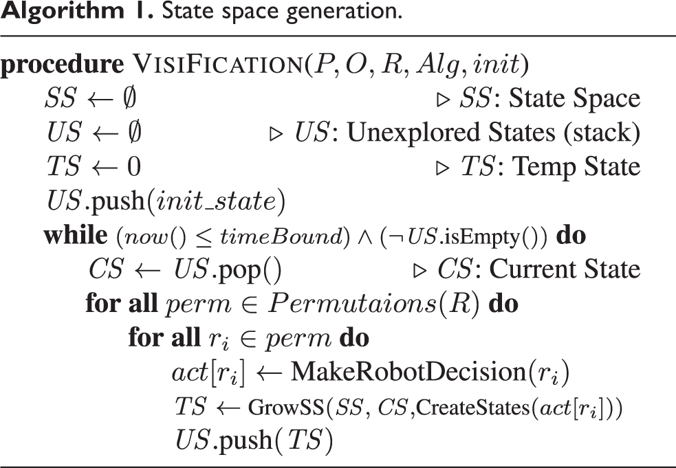
We have used Computational Geometry Algorithms Library³⁴ to implement the proposed method in C++.³⁵ The program automatically constructs the state space of the $M R S = (P, O, R, A l g, i n i t)$ during the movement of the robots. Precisely, the states and the transitions are constructed with respect to the decisions made by the robots during their movements (determined by the motion algorithms).

The pseudocode of the state space generation process is illustrated in Algorithm 1. At first, the initial state of the system is constructed ( $i n i t_s t a t e$ ) with respect to the initial positions of robots (init). At each permutation, each robot r_i makes the corresponding decision and moves toward the target. With respect to the robot decision, CreateStates returns the states obtained by taking action $a c t [r_{i}]$ based on the transition types described in the “Constructing the discrete state space” section. GrowSS extends the current generated state space (SS) with respect to current state CS and the returned states of CreateStates by generating only the new states and transitions which do not exist in SS. Since more than one event point may occur during the movement of r_i, CreateStates may construct more than one state (a chain of states) for action $a c t [r_{i}]$ . Because we consider all the permutations of robots to compute the next states, we may have a set of unexplored states called US which are explored in turn. Therefore, SS grows up gradually with respect to the movements of the robots. Due to the geometric complexity of the proposed method we do not provide the pseudocode of CreateStates function here, we refer the reader to the available online implementation³⁵ which contains the source code as well as a Debian-based package.

Algorithm 1. State space generation.

We analyze the proposed method based on two factors, the number of generated states and the convergence time (minutes). The number of generated states shows how complex MRS is modeled, and the convergence time indicates that how long does it take for the state space generation algorithm to converge and does not generate any new state. Precisely, in order to obtain the convergence time, we let the state space generation algorithm run for a significant amount of time to be sure that no new state is generated.

In the following subsections, we discuss two case studies (1) robots move based on Alpha algorithm³⁶ within polygonal domains with some restrictions on their movements (e.g. robots are only allowed to choose from some fixed movement directions) and (2) robots move freely based on a decentralized swarm aggregation algorithm²¹ within environments with obstacles. Our simulation environment is an Ubuntu 14.04 machine, Intel Pentium CPU 2.6 GHz with 4 GB RAM.

Constrained movement

As the first case study, we consider robot swarms algorithms in which the robots use only local wireless connectivity information to achieve swarm aggregation. Particularly, we use the simplest Alpha algorithm which is examined using simulations and real robot experiments of previous studies^16,36,37, as the navigation algorithms of the robots in this simulation. The implemented Alpha algorithm focuses on maintaining the connectivity of the communication graph during the robots’ movements. Alpha algorithm performs based on the value of α which is given as a threshold number. For each robot, If the number of visible robots is above the value of α, it executes a random turn to avoid the swarm simply collapsing on itself, otherwise, it executes a 180° turn to avoid moving out of the swarm.

The environments used by Dixon et al.¹⁶ is discretized by means of a grid which lets the robots only move in four directions (up, down, left, and right) with a fixed value of movement distance (robots move discretely). We constrained the possible movement directions of our proposed method (which has no limitations on the angle of directions and the value of movement distance) to the four directions with a fixed value of movement distance (robots move continuously with distance equal to one unit) in order to compare the number of generated states.

Table 1 analyzes our proposed state space generation algorithm with respect to the environments depicted in Figure 10. From the number of states (or convergence time) perspective, in Polygon (II), the ratio of the number of generated states when the number of robots is three (r₁, r₂, and r₃) and four increases about twice in comparison with Polygon (I). So, as the geometry of the environment gets more complex, the number of robots plays an important role on the number of generated states.

Table 1.
Analysis of the generated state space for grid-constrained movements.

Environment # Robots # States Convergence time (min)

Polygon (I) 3 217 5.7

4 735 31

Polygon (II) 3 308 41.1

4 1895 131.2

Figure 10.
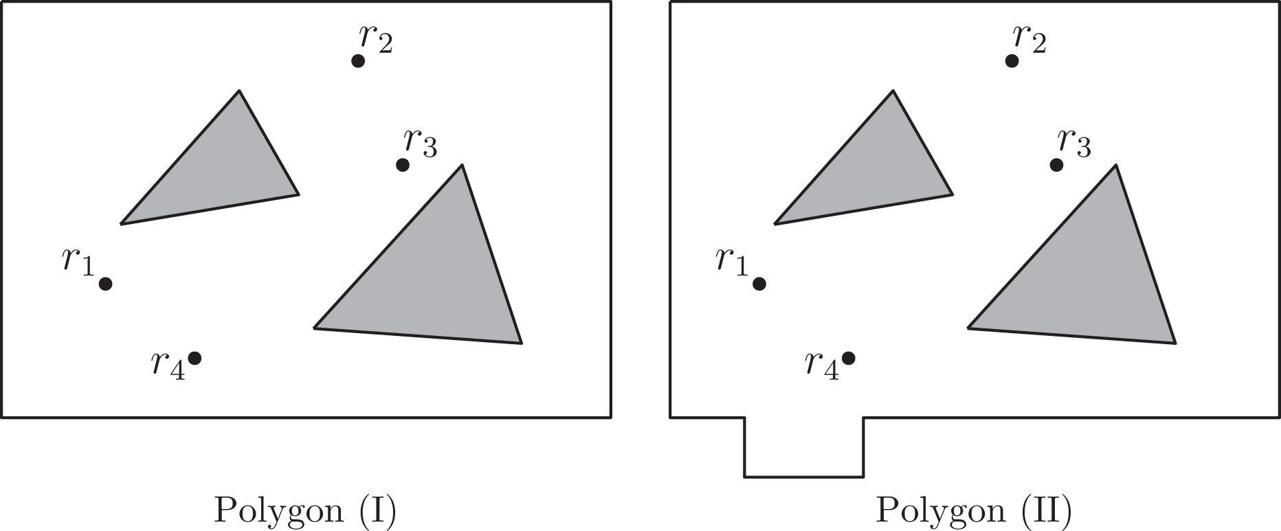
The polygon used for robots with grid-constrained movement.

Dixon et al.¹⁶ implemented the Alpha algorithm for three robots (k = 3) within grid sizes of 5 × 5 and 6 × 6 and obtained 168 × 10⁶ and 501 × 10⁶ number of states, respectively. Even though they completely abstracted out the geometry of the environment, the number of states achieved is considerably greater than the number of states computed by our method which let the robots move continuously in a geometric domain with obstacles.

In the previous work,²⁰ the motion of robots was restricted to only move along simple paths inside a simple polygon (with no obstacles inside). We put some limitations on our proposed method and constrain the possible movement directions of robots to two (left and right) over a given path in order to analyze the complexity of the generated state space. Table 2 examines the two state space-generation algorithms with respect to Figure 11 (obtained from O’Rourke⁵) where each robot is only allowed to traverse the corresponding path. As expected, the number of states computed by Sheshkalani et al.²⁰ is fewer than the number of states achieved in this work. In the previous work, in addition to $D G (S u b_{P})$ , they stored two (left and right) sequences for each robot (e.g. $S e q_{{\overset{\leftarrow}{m o v e}}_{r_{i}}}$ ) in order to indicate the sequence of intersection points of $W_{r_{i}}$ with vertices of Sub_P during traversing the corresponding path to the right. So, they only needed to compute the event points which may be reached when robot is moving to the left or right direction along the path in order to compute the successor states. Based on the state definition (Definition 5) sketched out in this work, which let the robots move freely inside the environment, we store the sequence of intersection points (by means of $D G (S u {b^{'}}_{P})$ ) in such a way that the successor states can be obtained uniquely (Lemma 2) with any arbitrary direction the robots choose to move. So, with respect to path-constrained movement, the previous work achieved fewer number of states (more information is stored as the state definition in this work to let the robots move freely) and subsequently converges faster than the proposed method.

Table 2.
Analysis of the generated state space for path-constrained movement.

Sheshkalani et al.²⁰ The proposed method Robots # States Convergenc time (min)

Polygon (III) $r_{1}, r_{2}, r_{3}$ 150 0.7

194 5

$r_{2}, r_{3}, r_{4}$ 186 1.5

198 5.4

Figure 11.
The polygon used for robots with path-constrained movement.⁵

Free movement

As the second case study, we consider a decentralized swarm aggregation algorithm based on local interactions for MRS with an integrated obstacle avoidance²¹ in which robots can move freely inside environments with obstacles. Although they used the second smallest eigen value (e.g. the algebraic connectivity) of the Laplacian matrix of the robots’ communication graph in order to preserve the connectivity, they could not have any integration of a connectivity maintenance algorithm within the proposed control schema. So, further we show that how our proposed method can be applied to guarantee that the respecting property may be preserved during the robots’ movements. Their proposed algorithm was examined using simulations along with experimental results carried out with the SAETTA mobile robotic platform. We use the proposed aggregation control law²¹ for each robot r_i in our simulations as the navigation algorithm a_i within the environments containing some obstacles.

Considering Figure 12, the convergence time of the proposed state space generation algorithm for polygons (IV) and (V) is 5.8 and 10.9 min, respectively. The reason for which the convergence time of Polygon (V) takes longer than Polygon (IV) is described as follows. As shown in Polygon (V), the robots are not visible to each other. So, at the beginning of the movement, each robot tries locally to find other robots in order to make the communication graph connected. This way, it takes more time for the robots to aggregate, and consequently maintain the connectivity in comparison with Polygon (IV), where the communication graph of robots is initially connected.

Figure 12.
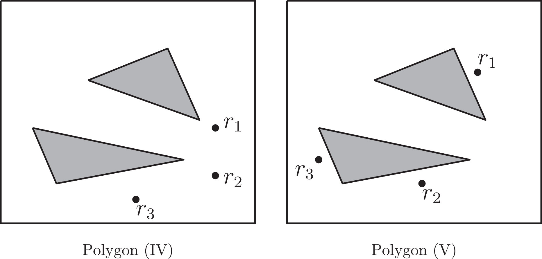
The polygons used for the robots with free movement.

We used the CADP²³ model-checker to verify the requirements (e.g. expressed in LTL_f formulas) regarding the generated state space. CADP evaluates each formula in less than 2 s which shows the applicability of the proposed method. Since the state space is constructed based on the given MRS, the verification method has to be rerun upon changes to MRS (e.g. navigation algorithms or initial position of robots). Figure 13 depicts an overall view of the automated verification process of an MRS. Table 3 shows the results of the verification process with respect to the environments depicted in Figure 12 and the mentioned LTL_f formulas. Recall that in the following, the LTL modalities □ and ⋄ are interpreted according to LTL_f semantics. The first formula □Connectivity, which is a safety property, indicates whether the communication graph of the robots is connected until the end of the trace and never gets violated. The second formula ⋄□Connectivity, which may reveal an important feature of Leccese et al.,²¹ is True; if eventually after some amount of time the robots become connected, and from then on, they always preserve the connectivity. The third formula ⋄Connectivity is True, if the robots are eventually connected which means that the communication graph does not always stay disconnected. According to LTL_f semantics, the second formula (persistence property) is equivalent to say that the last point in the trace satisfies Connectivity, that is, it is equivalent to $⋄ (L a s t \land C o n n e c t i v i t y)$ .²⁸ The last formula $⋄ (C o n n e c t i v i t y \land C o v e r a g e)$ is True, if the system eventually reaches a state in which the communication graph is connected and the environment is fully covered by the robots which may be considered as a goal state.

Figure 13.
The overall view of the automated verification process of an MRS. MRS: multi-robot system.

Table 3.
The results of the verification of two LTL_f formulas for free movement.

LTL_f formulas Polygon (IV) Polygon (V)

□Connectivity True False

⋄□Connectivity True True

⋄Connectivity True True

$⋄ (C o n n e c t i v i t y \land C o v e r a g e)$ False False

LTL: linear temporal logic.

Consider the polygons of Figure 12. Based on the initial positions of robots in Polygon (IV), the corresponding communication graph is connected. As stated in Table 3, the formula □Connectivity is True, which means that the underlying aggregation control law always preserves the global connectivity during the robots’ movements. On the other hand, robots’ positions in Polygon (V) show that the communication graph of robots is not initially connected which makes the mentioned formula False. Although Connectivity property is violated at first, as time goes by, the robots try to find each other and obtain the connectivity with respect to the navigation algorithms. In contrast to □Connectivity, the formula ⋄□Connectivity is satisfied in regard to Polygon (V) which shows that the proposed aggregation control law²¹ guarantees to maintain the connectivity as soon as the communication graph of robots becomes connected.

In the conclusions of Leccese et al.²¹ work, it is mentioned that they will focus on the integration of a connectivity maintenance algorithm within the proposed control schema. To the best of our knowledge, no contribution has been published to address the mentioned issue yet. Using our method, they can guarantee that the communication graph of robots is connected during the robots’ movements regarding the MRS and the desired LTL_f formula.

Conclusions

We presented a method to construct a discrete state space for an MRS and then verify the correctness properties by means of model-checking techniques. The notion of state has been defined in such a way that each state can be uniquely labeled with the atomic propositions Connectivity and Coverage. An important aspect of our method is that it treats the navigation algorithms as black boxes. Iteratively searching for new states, at each step, our algorithm asks the black box for its next action and creates the states caused by the action based on a precise definition of transitions. Using our provided implementation, the modeler can code the navigation algorithms and generate the state space. The generated state space is used to verify temporal formulas constructed over the mentioned propositions using the CADP tool. An important benefit of this approach is to eliminate the need for analytical proof of correctness upon changes to the navigation algorithms.

Since the robots’ initial positions have an influence on the verification results, it would be beneficial to suggest some specific regions of the environment as the possible robots’ initial positions have the potential to make the given temporal formulas satisfied. Future work will be focused on adding a preprocessing phase that subdivides the environment with respect to the formulas and let the modeler choose the initial positions from the suggested regions.

Environment	# Robots	# States	Convergence time (min)
Polygon (I)	3	217	5.7
4	735	31
Polygon (II)	3	308	41.1
4	1895	131.2

Sheshkalani et al.²⁰ The proposed method	Robots	# States	Convergenc time (min)
Polygon (III)	$r_{1}, r_{2}, r_{3}$	150	0.7
194	5
$r_{2}, r_{3}, r_{4}$	186	1.5
198	5.4

LTL_f formulas	Polygon (IV)	Polygon (V)
□Connectivity	True	False
⋄□Connectivity	True	True
⋄Connectivity	True	True
$⋄ (C o n n e c t i v i t y \land C o v e r a g e)$	False	False

Footnotes

Declaration of conflicting interests

The author(s) declared no potential conflicts of interest with respect to the research, authorship, and/or publication of this article.

Funding

The author(s) received no financial support for the research, authorship, and/or publication of this article.

ORCID iD

Ali Narenji Sheshkalani

References

Davison

Kita

. Active visual localisation for cooperating inspection robots. In: Proceedings of the IEEE/RSJ international conference on intelligent robots and systems 2000, Vol. 3, pp. 1709–1715. Takamatsu, Japan

Beard

McLain

Nelson

. Decentralized cooperative aerial surveillance using fixed-wing miniature UAVs. Proc IEEE 2006; 94(7): 1306–1324.

Sugiyama

Tsujioka

Murata

. Collaborative movement of rescue robots for reliable and effective networking in disaster area. In: Proceedings of the international conference on collaborative computing: networking, applications and worksharing. pp. 1306–1324, 2005.

Cannell

Stilwell

. A comparison of two approaches for adaptive sampling of environmental processes using autonomous underwater vehicles. In: Proceedings of OCEANS 2005 MTS/IEEE, Washington, DC, USA, 17–23 September 2005, Vol. 2, pp. 1514–1521.

O’Rourke

. Art gallery theorems and algorithms. Vol. 57. Oxford: Oxford University Press, 1987.

Durocher

Filtser

Fraser

. A (7/2)-approximation algorithm for guarding orthogonal art galleries with sliding cameras. In: LATIN 2014: theoretical informatics. Berlin: Springer, 2014, pp. 294–305. Berlin, Heidelberg: Springer.

Efrat

Leonidas

Har-Peled

. Sweeping simple polygons with a chain of guards. In: Proceedings of the eleventh annual ACM-SIAM symposium on discrete algorithms. San Francisco, California, USA, 9–11 January 2000, pp. 927–936.

Clarke

Grumberg

Peled

Model checking. Cambridge: MIT Press, 1999.

Fainekos

Kress-Gazit

Pappas

. Temporal logic motion planning for mobile robots. In: Proceedings of the IEEE international conference on robotics and automation, April 2005, pp. 2020–2025.

10.

Fainekos

Girard

Kress-Gazit

. Temporal logic motion planning for dynamic robots. Automatica 2009; 45(2): 343–352.

11.

Pnueli

. The temporal logic of programs. In: 18th annual symposium on foundations of computer science, October 1977, pp. 46–57. Piscataway: IEEE, 1977.

12.

Liu

Winfield

AFT

. Modeling and optimization of adaptive foraging in swarm robotic systems. Int J Rob Res 2010; 29(14): 1743–1760.

13.

Konur

Dixon

Fisher

. Analysing robot swarm behaviour via probabilistic model checking. Robot Auton Syst 2012; 60(2): 199–213.

14.

Hinton

Kwiatkowska

Norman

. PRISM: A tool for automatic verification of probabilistic systems. In: Proceedings of the 12th international conference on tools and algorithms for the construction and analysis of systems. Berlin: Springer, 2006, pp. 441–444. Berlin, Heidelberg: Springer.

15.

Kloetzer

Belta

. Temporal logic planning and control of robotic swarms by hierarchical abstractions. IEEE Trans Robot 2007; 23: 320–330.

16.

Dixon

Winfield

Fisher

. Towards temporal verification of swarm robotic systems. Robot Auton Syst 2012; 60(11): 1429–1441.

17.

Brambilla

Brutschy

Dorigo

. Property-driven design for robot swarms: a design method based on prescriptive modeling and model checking. ACM Trans Auton Adap Sys 2014; 9(4): 17.

18.

Guo

Dimarogonas

. Distributed plan reconfiguration via knowledge transfer in multi-agent systems under local LTL specifications. In: Robotics and automation (ICRA), IEEE international conference, May 2014, pp. 4304–4309.

19.

Sheshkalani

Khosravi

Fallah

. Discretizing the state space of multiple moving robots to verify visibility properties. In: Conference towards autonomous robotic systems. Berlin: Springer, 2015, pp. 186–191. Cham, Switzerland: Springer International Publishing.

20.

Sheshkalani

Khosravi

Mohammadi

. Verification of visibility-based properties on multiple moving robots. In: Conference towards autonomous robotic systems. Berlin: Springer, 2017, pp. 51–65. Cham, Switzerland: Springer International Publishing.

21.

Leccese

Gasparri

Priolo

. A swarm aggregation algorithm based on local interaction with actuator saturations and integrated obstacle avoidance. In: IEEE international conference on robotics and automation, May 2013, pp. 1865–1870.

22.

Sabattini

Secchi

Chopra

. Decentralized estimation and control for preserving the strong connectivity of directed graphs. IEEE Trans Cybern 2015; 45(10): 2273–2286.

23.

Garavel

Lang

Mateescu

. CADP 2010: a toolbox for the construction and analysis of distributed processes. In: International conference on tools and algorithms for the construction and analysis of systems. Berlin, Heidelberg: Springer, 2011, pp. 372–387.

24.

Ghosh

SK.

Visibility algorithms in the plane. Cambridge: Cambridge University Press, 2007.

25.

Antuña

Araiza-Illan

Campos

. Symmetry reduction enables model checking of more complex emergent behaviours of swarm navigation algorithms. In: Towards autonomous robotic systems—16th annual conference, proceedings 2015, pp. 26–37. Cham, Switzerland: Springer International Publishing.

26.

Peled

Vardi

Yannakakis

. Black box checking. J Autom Lang Comb 2001; 7(2): 225–246.

27.

Baier

Katoen

. Principles of model checking. Cambridge: MIT Press, 2008

28.

De Giacomo

Vardi

. Linear temporal logic and linear dynamic logic on finite traces. In: Proceedings of the twenty-third international joint conference on artificial intelligence IJCAI ‘13, Beijing, China, pp. 854–860. AAAI Press.

29.

De Giacomo

De Masellis

Montali

. Reasoning on LTL on finite traces: insensitivity to infiniteness. In: Proceedings of the twenty-eighth aaai conference on artificial intelligence AAAI’14, pp. 1027–1033. AAAI Press.

30.

Eisner

Fisman

Havlicek

. Reasoning with temporal logic on truncated paths. In: Computer aided verification. Heidelberg: Springer, 2003, pp. 27–39.

31.

Keller

. Formal verification of parallel programs. Commun ACM 1976; 19(7): 371–384.

32.

Shamos

Hoey

. Geometric intersection problems. In: Foundations of computer science, 17th annual symposium, October 1976, pp. 208–215. Piscataway: IEEE.

33.

Mirante

Weingarten

. The radial sweep algorithm for constructing triangulated irregular networks. IEEE Comput Graph Appl 1982; 2(3): 11–21.

34.

Hemmer

Huang

Bungiu

. 2D visibility computation. In: CGAL user and reference manual. 4.7 ed. CGAL Editorial Board, 2015.

35.

Sheshkalani

Khosravi

Mohammadi

. Verification of visibility-based properties on multiple moving robots in an environment with obstacles, https://gitlab.com/narenji/VisiFication (2017, accessed 17 March 2018).

36.

Nembrini

Winfield

Melhuish

. Minimalist coherent swarming of wireless networked autonomous mobile robots. In: Proceedings of the seventh international conference on simulation of adaptive behavior on from animals to animats, 2002, pp. 373–382. ICSAB, Cambridge: MIT Press.

37.

Winfield

Liu

Nembrini

. Modelling a wireless connected swarm of mobile robots. Swarm intelligence 2008; 2(2–4): 241–266.