Sage Journals: Discover world-class research

Abstract

This article deals with using of geometric mechanics at modeling mixed mechanical locomotion systems. In introductory part, the division of locomotion systems and reduced motion equation, which create the mathematical model of the system, is analyzed. Further we devoted to example of mixed locomotion system—two-link snake. We created the mathematical model of this example, simulated this system, and represented other tools of geometric mechanics.

Keywords

Two-link snake nonholonomic constraint Lagrangian mathematical model vector field gait height and gamma function

Introduction

Mathematical modeling is interesting for engineers in the process of designing devices and systems. Thus, engineers should be able to create description of the system to be able to predict the system behavior before its realization. The classical modeling of multibody systems (e.g. Lagrangian mechanics) leads to complicated equations of motion and these equations are often not suitable for control design. In this article, we focused on tools of geometric mechanics that provide a better tool for creating motion equations and better understanding of their dynamics.

At writing this article, we were inspired by the works of Hatton and Choset,^1,2 Ebetiuc and Harald,³ Shammas et al.,⁴ and Karavaev and Kilin,⁵ who devoted mathematical modeling of locomotion systems using geometric mechanics. The locomotion of system is based on change of system shape that provides total motion of system as we can see in Figure 1 on motion of cat. In the work of Lipták et al.,⁶ we devoted three-link snake-like robot. This three-link snake-like robot belongs to the category of principally kinematic systems. We dealt with the proposal of gait for sidewinding movement of snake for ensuring maximal net motion.

Figure 1.

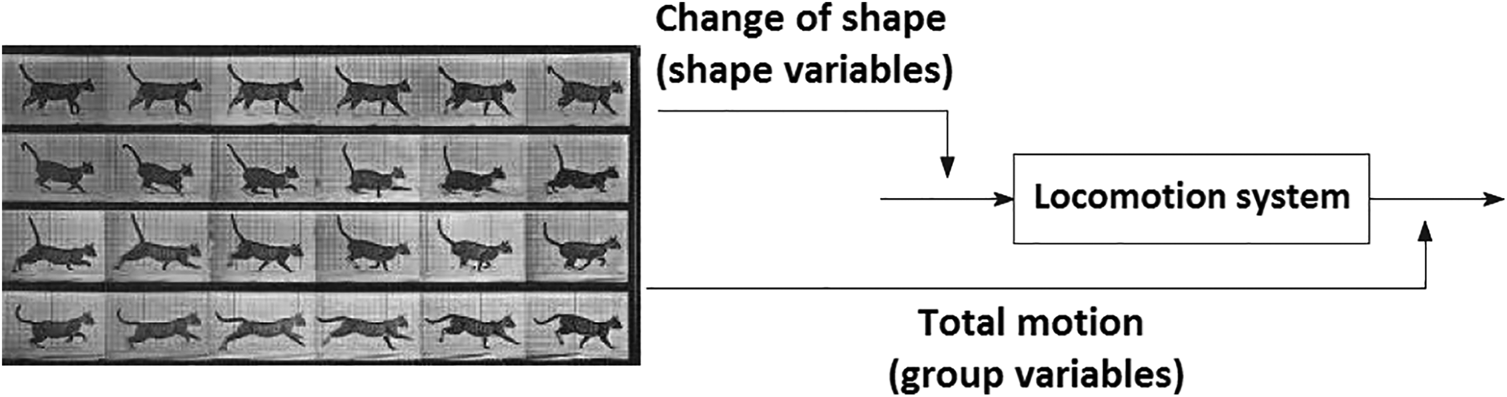
Scheme of locomotion principle.

In this article, we show the locomotion on example of two-link snake-like robot. This snake belongs to different category—mixed systems; it has a different mathematical model and different way of creating its model. Here is used a different gait that generates the lateral movement of snake and we describe modes how the two-link snake moves only using one action variable.

Generalized mixed mechanical locomotion system

Generalized mixed locomotion system represents a simple mechanical system that has n-dimensional configuration space with trivial principal fiber bundle structure Q = G × M, where G is l-dimensional fiber space with Lie group structure and M is m-dimensional base (shape) space that is subjected to k nonholonomic constraints. These systems should apply the following:

1. Its Lagrangian consists only of kinetic energy

L (q, \dot{q}) = \frac{1}{2} {\dot{q}}^{T} M (q) \dot{q}

where M(q) is n × n mass matrix that defines metric bases on kinetic energy.

2. Nonholonomic constraints that act to mechanical system are expressed in Pfaffian form

ω (q) \dot{q} = 0

where ω(q) is k × n matrix that describes nonholonomic constraints.

3. Lagrangian and nonholonomic constraints are G-invariant (with respect to actions of Lie group)

L (q, \dot{q}) = L (Φ_{g} q, T_{q} Φ_{g} \dot{q})

ω (q) \dot{q} = ω (Φ_{g} q) T_{q} Φ_{g} \dot{q}

where Φ_g is action of Lie group to Q and T_qΦ_g is lifted action on tangent bundle TQ.

4. Nonholonomic constraints are linearly independent, that is, none of nonholonomic constraints are a linear combination of other nonholonomic constraints.⁷

In general, reduced motion equations of generalized mixed systems consist of three types of equation

ξ^{b} = T_{g} L_{g^{- 1}} \dot{g} = - A (r) \dot{r} + I^{- 1} p^{T}

\dot{p} = \frac{1}{2} {\dot{r}}^{T} σ_{\dot{r} \dot{r}} (r) \dot{r} + p^{T} σ_{p \dot{r}} (r) \dot{r} + \frac{1}{2} p^{T} σ_{p p} (r) p

M \ddot{r} + {\dot{r}}^{T} C (r) \dot{r} + N (r, \dot{r}, p) = τ (r)

Equation (6) is called as reconstruction equation and is used to solve body fiber velocities ξ^b (or word fiber velocities $\dot{g}$ ) for given base configuration A(r), base velocities $\dot{r}$ , and momentum p. Momentum equation (7) describes evolution of momentum and reduced base dynamic equation (8) expresses evolution of base (shape) variables. Equations (6) and (7) are set of l first-order differential equation and equation (8) is set of m second-order differential equation. The relation among individual equation can be seen in Figure 2.⁷

Figure 2.

Block diagram of reduced motion equations.

By defining other conditions to dimension of fiber and base subspace and number of nonholonomic constraints, we get subtypes of locomotion systems presented in the following table (Figure 3).

Figure 3.

Subtypes of generalized mixed locomotion systems.⁷

In this article, we will discuss one subtype of generalized mixed mechanical systems—the mixed mechanical system. We will show how to build the mathematical model (reduced motion equations) for chosen mechanical system (the two-link snake) and how to control the system by method of gait proposal.

Mixed mechanical locomotion system

Mixed mechanical locomotion systems that belong to generalized mixed locomotion systems apply the following:

These systems have at least one nonholonomic constraint.

They have maximally about one nonholonomic constraint less than the dimension of fiber space, that is, 0 < k < l, where l is the dimension of fiber space and k is the number of nonholonomic constraints.

They are mechanical systems that do not have enough nonholonomic constraints to define span of group space.^7,8

The locomotion of two-link snake will be created by changing the angle size α₁. The position and orientation of two-link snake in-plane is described using three fiber variables (x, y, θ) ∊ SE(2) and configuration space of snake has the form

Q = G \times M = S E (2) \times S

This two-link snake (Figure 4) belongs according to the dimension of base space to the category of purely dynamic systems, because its base space is one-dimensional. But to build the reconstruction equation except nonholonomic constraints, we need to use also generalized momentum, because the number of nonholonomic constraints k = 2 is smaller than the dimension of fiber space l = 3. Because of this, the two-link snake is included to the category of mixed mechanical systems.

Figure 4.

The simplified model of two-link snake.

Nonholonomic constraints and Lagrangian

In this section, we need to derive nonholonomic constraints and the Lagrangian of two-link snake and review their G-invariance.

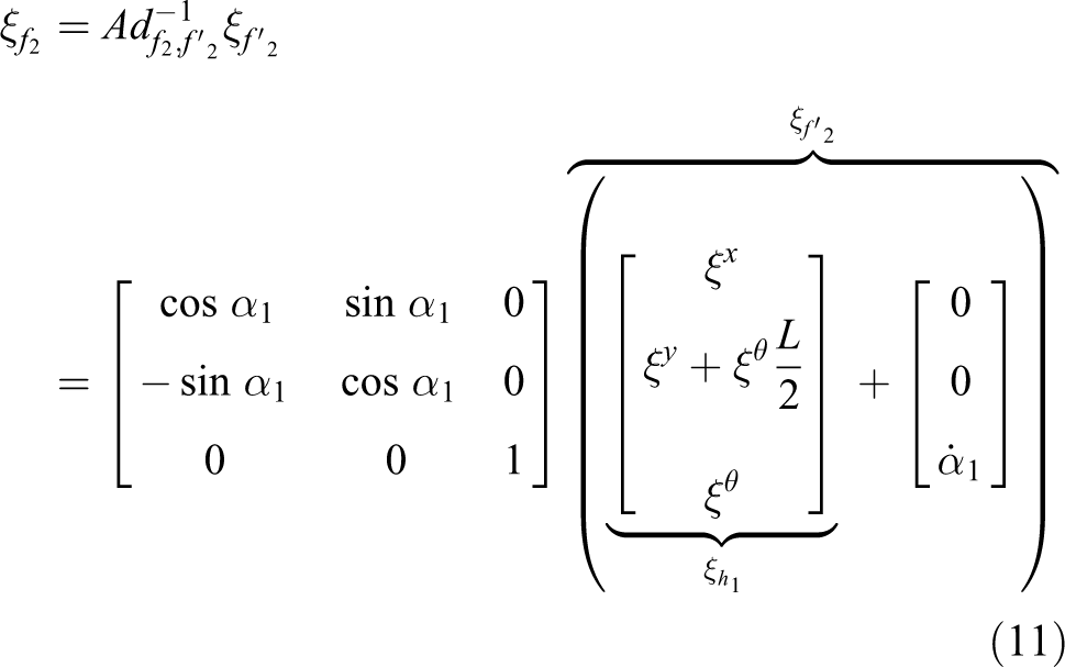
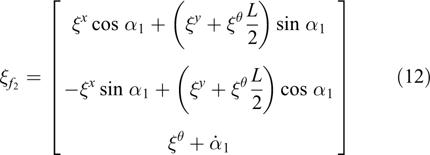
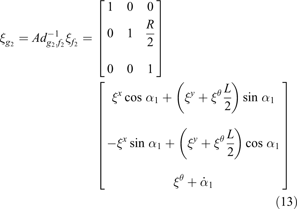
For two-link snake, we have two nonholonomic constraints, which we derive using adjoint action. The body velocity of the mass center of the first link has the form

ξ_{g_{1}} = [\begin{matrix} ξ^{x} \\ ξ^{y} \\ ξ^{θ} \end{matrix}]

In order to calculate the body velocity of the second link in its center of mass, at first we have to determine the body velocity of the end of the first link as is shown in Figure 5 ¹

ξ_{h_{1}} = A d_{h_{1}, g_{1}}^{- 1} ξ_{g_{1}} = [\begin{matrix} cos θ & sin θ & x sin θ - y cos θ \\ - sin θ & cos θ & x cos θ + y sin θ \\ 0 & 0 & 1 \end{matrix}] ξ_{g_{1}} = [\begin{matrix} 1 & 0 & 0 \\ 0 & 1 & \frac{L}{2} \\ 0 & 0 & 1 \end{matrix}] [\begin{matrix} ξ^{x} \\ ξ^{y} \\ ξ^{θ} \end{matrix}] = [\begin{matrix} ξ^{x} \\ ξ^{y} + ξ^{θ} \frac{L}{2} \\ ξ^{θ} \end{matrix}]

Figure 5.

Showing of individual frames of two-link snake.

Other velocities are determined by the same manner

ξ_{f_{2}} = A d_{f_{2}, {f^{'}}_{2}}^{- 1} ξ_{{f^{'}}_{2}} = [\begin{matrix} \cos α_{1} & \sin α_{1} & 0 \\ - \sin α_{1} & \cos α_{1} & 0 \\ 0 & 0 & 1 \end{matrix}] \overset{}{\overset{}{\overset{ξ_{{f^{'}}_{2}}}{\overset{︷}{(\underset{}{\underset{}{\underset{ξ_{h_{1}}}{\underset{︸}{[\begin{matrix} ξ^{x} \\ ξ^{y} + ξ^{θ} \frac{L}{2} \\ ξ^{θ} \end{matrix}]}}}} + [\begin{matrix} 0 \\ 0 \\ {\dot{α}}_{1} \end{matrix}])}}}}

ξ_{f_{2}} = [\begin{matrix} ξ^{x} cos α_{1} + (ξ^{y} + ξ^{θ} \frac{L}{2}) sin α_{1} \\ - ξ^{x} sin α_{1} + (ξ^{y} + ξ^{θ} \frac{L}{2}) cos α_{1} \\ ξ^{θ} + {\dot{α}}_{1} \end{matrix}]

ξ_{g_{2}} = A d_{g_{2}, f_{2}}^{- 1} ξ_{f_{2}} = [\begin{matrix} 1 & 0 & 0 \\ 0 & 1 & \frac{R}{2} \\ 0 & 0 & 1 \end{matrix}] [\begin{matrix} ξ^{x} cos α_{1} + (ξ^{y} + ξ^{θ} \frac{L}{2}) sin α_{1} \\ - ξ^{x} sin α_{1} + (ξ^{y} + ξ^{θ} \frac{L}{2}) cos α_{1} \\ ξ^{θ} + {\dot{α}}_{1} \end{matrix}]

ξ_{g_{2}} = [\begin{matrix} ξ^{x} cos α_{1} + (ξ^{y} + ξ^{θ} \frac{L}{2}) sin α_{1} \\ - ξ^{x} sin α_{1} + \frac{R}{2} (ξ^{θ} + {\dot{α}}_{1}) + (ξ^{y} + ξ^{θ} \frac{L}{2}) \\ ξ^{θ} + {\dot{α}}_{1} \end{matrix} cos α_{1}]

For the first and second links of snake, we have no-slip condition in the y-direction expressed in body coordinates

ξ_{g_{1}}^{y} = 0 and ξ_{g_{2}}^{y} = 0

ξ^{y} = 0

- ξ^{x} sin α_{1} + \frac{R}{2} (ξ^{θ} + {\dot{α}}_{1}) + (ξ^{y} + ξ^{θ} \frac{L}{2}) cos α_{1} = 0

and these conditions can be rewritten into Pfaffian form

[\begin{matrix} 0 & 1 & 0 & 0 \\ - sin α_{1} & cos α_{1} & \frac{R}{2} + \frac{L}{2} cos α_{1} & \frac{R}{2} \end{matrix}] [\begin{matrix} ξ^{x} \\ ξ^{y} \\ ξ^{θ} \\ {\dot{α}}_{1} \end{matrix}] = [\begin{matrix} 0 \\ 0 \end{matrix}]

Using lifted action T_eL_g, these two nonholonomic constraints (16) and (17) can get the form in world coordinates

\dot{x} sin (θ + α_{1}) - \dot{y} cos (θ + α_{1}) - \dot{θ} (\frac{R}{2} + \frac{L}{2} cos α_{1}) - \frac{R}{2} {\dot{α}}_{1} = 0

\dot{x} sin θ - \dot{y} cos θ = 0

Nonholonomic constraints are not linearly dependent, that is, they are G-invariant.

The simplified shape of Lagrangian will be expressed with respect to coordinates x and y, taking into account the different lengths of links L and R, thus also weights m_L and m_R and the inertia of individual links J_L and J_R . Different lengths of links were chosen because of nonzero resulting torque after acting input variable in the joint as we can see in Figure 6. In the case of cyclic gaits with the same length of links, there would be no locomotion of the two-link snake because the resulting torque would be equal to zero.

Figure 6.

Showing of propulsive force F and individual torques M_L and M_R acting to two-link snake.

The Lagrangian of snake has the form

L (q, \dot{q}) = \frac{1}{2} (m_{L} + m_{R}) ({\dot{x}}^{2} + {\dot{y}}^{2}) + \frac{1}{2} (J_{L} + J_{R}) {\dot{θ}}^{2} + \frac{1}{2} J_{R} {(\dot{θ} + {\dot{α}}_{1})}^{2}

and now we verify the G-invariance of Lagrangian using left action of Lie group Φ_g and lifted action T_qΦ_g

Φ_{g} q = (u + x cos α - y sin α, v + x sin α + y cos α, θ + α, α_{1})

T_{q} Φ_{g} \dot{q} = (\dot{x} cos α - \dot{y} sin α, \dot{x} sin α + \dot{y} cos α, \dot{θ}, {\dot{α}}_{1})

After substituting Lie group and lifted action to the Lagrangian equation (21), we get the same form of Lagrangian, that is, Lagrangian is G-invariant

L (q, \dot{q}) = L (Φ_{g}, T_{q} Φ_{g})

Reconstruction equation

When Lagrangian and nonholonomic constraints are G-invariant, then reduced Lagrangian and reduced nonholonomic constraints are expressed as^1,7

l (r, ξ, \dot{r}) = \frac{1}{2} {[\begin{matrix} ξ & \dot{r} \end{matrix}]}^{T} [\begin{matrix} I & I A \\ {(I A)}^{T} & m \end{matrix}] [\begin{matrix} ξ \\ \dot{r} \end{matrix}] = \frac{1}{2} {ξ^{T} I ξ + 2 {\dot{r}}^{T} {(I A)}^{T} ξ + {\dot{r}}^{T} m \dot{r}}

[\begin{matrix} {\bar{ω}}_{ξ} & {\bar{ω}}_{\dot{r}} \end{matrix}] [\begin{matrix} ξ \\ \dot{r} \end{matrix}] = 0

where I is the local form of locked inertia tensor in body coordinates, A is the local form of mechanical connection, and $ω_{ξ} and ω_{\dot{r}}$ are the submatrices of matrix of nonholonomic constraints.

Reduced Lagrangian for two-link snake is

l (r, ξ, \dot{r}) = \frac{1}{2} {[\begin{matrix} ξ^{x} \\ ξ^{y} \\ ξ^{θ} \\ {\dot{α}}_{1} \end{matrix}]}^{T} [\begin{matrix} (m_{L} + m_{R}) & 0 & 0 & 0 \\ 0 & (m_{L} + m_{R}) & 0 & 0 \\ 0 & 0 & (J_{L} + J_{R}) & J_{R} \\ 0 & 0 & J_{R} & J_{R} \end{matrix}] [\begin{matrix} ξ^{x} \\ ξ^{y} \\ ξ^{θ} \\ {\dot{α}}_{1} \end{matrix}]

At first, we must determine kinematic distribution D_q using nonholonomic constraints according to relation^9
–11

D_{q} = span {\partial_{α_{1}}, a \partial_{x} + b \partial_{y} + c \partial_{θ}}

where a, b, and c are coefficients at group variables $ξ^{x}, ξ^{y}, a n d ξ^{θ}$ , that we get by editing nonholonomic constraints, thus substituting equation (16) to equation (17)

ξ^{x} \underset{a}{\underset{︸}{\sin α_{1}}} \underset{}{} + ξ^{y} \underset{b}{\underset{︸}{0}} + ξ^{θ} \underset{c}{\underset{︸}{\underset{}{(- \frac{L}{2} \cos α_{1} - \frac{R}{2})}}} - \frac{R}{2} {\dot{α}}_{1} = 0

The tangent bundle to the orbits of SE (2) action is given by

T_{q} (Orb (q)) = span {\partial_{x}, \partial_{y}, \partial_{θ}}

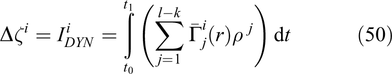
The intersection between tangent bundle to group orbits and distribution of constraints is section S_q (Figure 7)

S_{q} = D_{q} \cap T_{q} (O r b (q)) = s p a n {a \partial_{x} + b \partial_{y} + c \partial_{θ}}

Figure 7.

The intersection between tangent bundle and distribution.⁹

The nonholonomic momentum can be constructed by selecting section S_q that has the form as a bundle over Q. Because section S_q is one-dimensional, this section can be determined as

ξ_{Q}^{q} = a \partial_{x} + b \partial_{y} + c \partial_{θ}

and is invariant under group action SE on Q. The nonholonomic momentum of two-link snake is⁹

p = \frac{\partial l}{\partial ξ^{i}} {(ξ_{Q}^{q})}^{i} = sin α_{1} (m_{L} + m_{R}) ξ^{x} + (- \frac{L}{2} cos α_{1} - \frac{R}{2}) (J_{L} + 2 J_{R}) ξ^{θ} + (- \frac{L}{2} cos α_{1} - \frac{R}{2}) J_{R} {\dot{α}}_{1}

Nonholonomic constraints (16) and (17) and nonholonomic momentum (33) we express in Pfaffian form

[\begin{matrix} 0 \\ 0 \\ p \end{matrix}] = [\begin{matrix} sin α_{1} & - cos α_{1} & - \frac{L}{2} cos α_{1} - \frac{R}{2} & - \frac{R}{2} \\ 0 & 1 & 0 & 0 \\ sin α_{1} (m_{L} + m_{R}) & 0 & - \frac{L}{2} cos α_{1} - \frac{R}{2} (J_{L} + 2 J_{R}) & - \frac{L}{2} cos α_{1} - \frac{R}{2} J_{R} \end{matrix}] [\begin{matrix} ξ^{x} \\ ξ^{y} \\ ξ^{θ} \\ {\dot{α}}_{1} \end{matrix}]

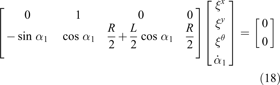
and then we create the reconstruction equation of snake-like robot

ξ = \underset{}{\underset{}{\frac{1}{D} \underset{A}{\underset{︸}{[\begin{matrix} (\frac{L}{2} \cos α_{1} + \frac{R}{2}) (R (J_{L} + J_{R}) - J_{R} L \cos α_{1}) \\ 0 \\ R \sin α_{1} (m_{L} + m_{R}) - 2 J_{R} \sin α_{1} (\frac{L}{2} \cos α_{1} + \frac{R}{2}) \end{matrix}]}}}} \dot{r} + \underset{}{\underset{}{\underset{I^{- 1}}{\underset{︸}{\frac{1}{D} [\begin{matrix} - L \cos α_{1} - R \\ 0 \\ - \sin α_{1} \end{matrix}]}}} p}

where $D = sin α_{1} (L cos α_{1} + R) (J_{L} + 2 J_{R} - m_{L} - m_{R})$ and $\dot{r} = {\dot{α}}_{1}$ .

Momentum evolution equation

In this part, we will express the equation describing momentum evolution. We get this equation based on relation⁹

\dot{p} = \frac{\partial l}{\partial ξ^{i}} {[\frac{d}{dt} (ξ^{q})]}_{Q}^{i}

\dot{p} = sin α_{1} (m_{L} + m_{R}) ξ^{x} cos α_{1} {\dot{α}}_{1} + (- \frac{L}{2} cos α_{1} - \frac{R}{2}) (J_{L} + 2 J_{R}) ξ^{θ} \frac{L}{2} sin α_{1} {\dot{α}}_{1} + (- \frac{L}{2} cos α_{1} - \frac{R}{2}) J_{R} {\dot{α}}_{1} \frac{L}{2} sin α_{1} {\dot{α}}_{1}

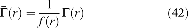
Because of simplifying momentum, we establish the new variable scaled momentum defined as⁷

ρ = f (r) p

where f is the integrating factor of the first-order differential equation. Then, the momentum evolution equation has the following form

\dot{ρ} = {\dot{r}}^{T} \sum (r) \dot{r} = f (r) ({\dot{r}}^{T} σ_{\dot{r} \dot{r}} \dot{r})

for our example

\dot{ρ} = \underset{}{\underset{}{\underset{f (r)}{\underset{︸}{J_{R} \frac{L}{2} \sin α_{1}}}} \underset{{\dot{r}}^{T} σ_{\dot{r} \dot{r}} \dot{r}}{\underset{︸}{\underset{}{{\dot{α}}_{1} (- \frac{L}{2} \cos α_{1} - \frac{R}{2}) {\dot{α}}_{1}}}}} \underset{}{}

Thus, the reconstruction equation will have a new form

ξ = - A (r) \dot{r} + \bar{Γ} (r) ρ

where $\bar{Γ} (r)$ is calculated according to the following relation

\bar{Γ} (r) = \frac{1}{f (r)} Γ (r)

The final form of the reconstruction equation for two-link snake is

ξ = \underset{}{\underset{}{\frac{1}{D} \underset{A}{\underset{︸}{[\begin{matrix} (\frac{L}{2} \cos α_{1} + \frac{R}{2}) (R (J_{L} + J_{R}) - J_{R} L \cos α_{1}) \\ 0 \\ R \sin α_{1} (m_{L} + m_{R}) - 2 J_{R} \sin α_{1} (\frac{L}{2} \cos α_{1} + \frac{R}{2}) \end{matrix}]}}}} \dot{r} + \underset{}{\underset{}{\frac{1}{D} \underset{\bar{Γ}}{\underset{︸}{[\begin{matrix} \frac{2 (- L \cos α_{1} - R)}{J_{R} L \sin α_{1}} \\ 0 \\ - \frac{2}{J_{R} L} \end{matrix}]}}}} ρ

or expressed by world velocities

\dot{g} = \underset{}{\underset{}{\frac{1}{D} \underset{A}{\underset{︸}{[\begin{matrix} \cos θ (\frac{L}{2} \cos α_{1} + \frac{R}{2}) (R (J_{L} + J_{R}) - J_{R} L \cos α_{1}) \\ \sin θ (\frac{L}{2} \cos α_{1} + \frac{R}{2}) (R (J_{L} + J_{R}) - J_{R} L \cos α_{1}) \\ R \sin α_{1} (m_{L} + m_{R}) - 2 J_{R} \sin α_{1} (\frac{L}{2} \cos α_{1} + \frac{R}{2}) \end{matrix}]}}}} \dot{r} + \underset{}{\underset{}{\frac{1}{D} \underset{\bar{Γ}}{\underset{︸}{[\begin{matrix} \cos θ \frac{2 (- L \cos α_{1} - R)}{J_{R} L \sin α_{1}} \\ \sin θ \frac{2 (- L \cos α_{1} - R)}{J_{R} L \sin α_{1}} \\ - \frac{2}{J_{R} L} \end{matrix}]}}}} ρ

Representation of local connection using vector fields

The local connection A of snake is shown using vector fields in MATLAB because individual expressions of connection are complicated and do not provide insight into system behavior. We analyze shape of arrows of local connection with shape of generated gait that provides the locomotion of system.^12
–14 Individual parameters of snake links we get from SolidWorks are as follows: L = 0.162 m, R = 0.486 m, m_L = 0.0526 kg, m_R = 0.07488 kg, J_L = 0.01022 kgm², and J_R = 0.0199 kgm².

The gait ϕ that generates lateral movement of snake has the form

α_{1} = 0.698 sin t

Angular rotation of joint we get by differentiating angular rotation according to time

{\dot{α}}_{1} = 0.698 cos t

After defining the form of gait, we can show gait to individual vector fields.

From the following figures, we can deduce how the snake will move in individual coordinates x, y, and θ. We proceed according to the following rules:

When arrows of vector field ${\vec{A}}^{ξ_{x}}$ are disapprovingly oriented with generated gait (Figure 8), then the snake moves in negative direction, and in opposite situation, the snake moves in positive direction of coordinate x, arrows that are perpendicular to gait cause only rotation of snake.

Vector field of ${\vec{A}}^{ξ_{y}}$ is zero vector field (Figure 9), it implies from nonholonomic constraints.

Arrows of vector field ${\vec{A}}^{ξ_{θ}}$ that are parallel to gait produce only joint rotation of snake, and in perpendicular direction to gait, the snake does not rotate (Figure 10).

Figure 8.

The vector field of local connection ${\vec{A}}^{ξ_{x}}$ .

Figure 9.

The vector field of local connection ${\vec{A}}^{ξ_{y}}$ .

Figure 10.

The vector field of local connection ${\vec{A}}^{ξ_{θ}}$ .

Now we express the reconstruction equation and momentum equation of two-link snake using block diagram (Figure 11) and show the courses of individual components during one period (Figure 12).

Figure 11.

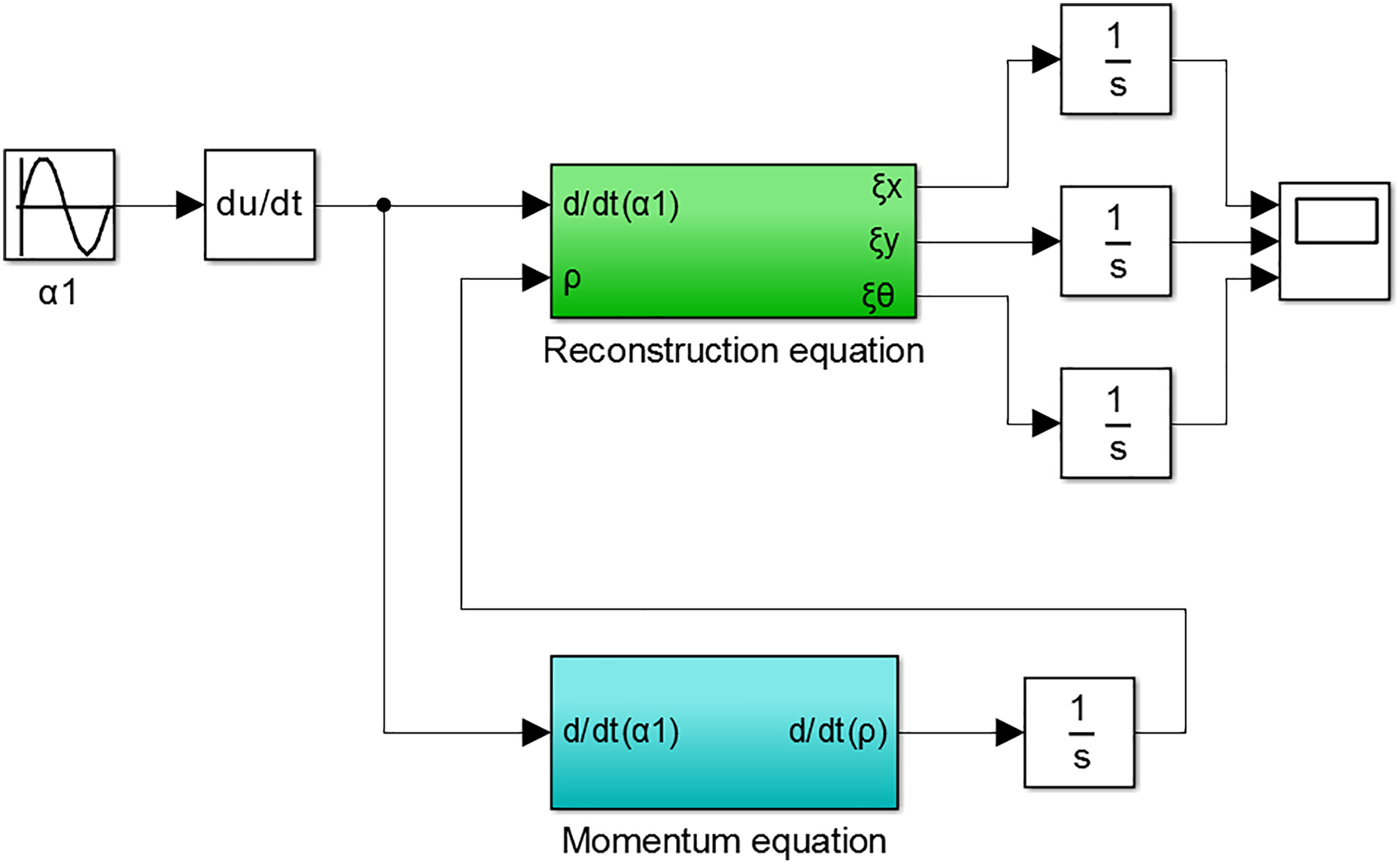
The block diagram of reconstruction equation expressed in the body velocities.

Figure 12.

The courses of individual components.

In the following, Figure 13 shows the lateral movement of snake simulated in SolidWorks.

Figure 13.

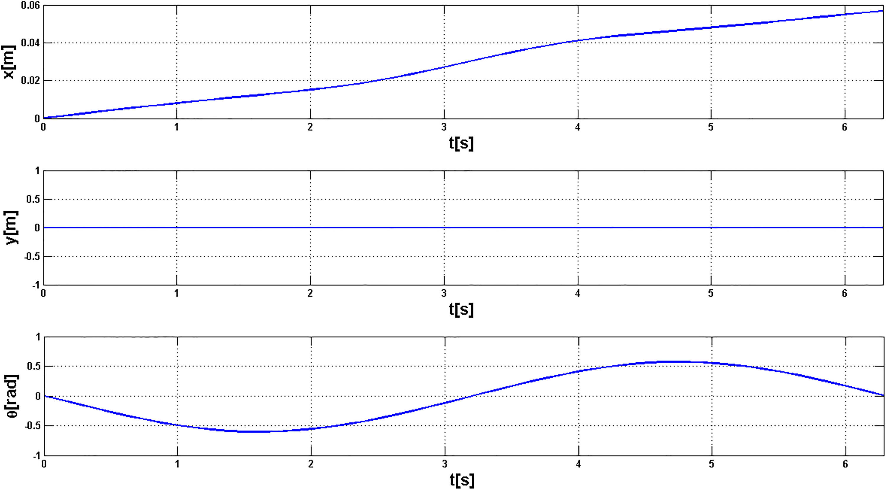
The lateral movement of snake with shown trajectory of mass center.

The distance that snake moves at lateral movement during one period is 83.86 mm where extension of the second link causes the increase in travelled distance. In the reverse configuration when the first link is longer than the second link, movement direction is reverse because the final momentum has a reverse orientation.

Height and gamma functions of two-link snake

The position change expressed in the body velocity for coordinates x, y, and θ is equal to the sum of geometric and dynamic phase shift^7,15,16

Δ ζ^{i} = I_{GEO}^{i} + I_{DYN}^{i}

where

I_{GEO}^{i} = \oint_{r (t_{0})}^{r (t_{1})} (- \sum_{j = 1}^{m} A_{j}^{i} (r)) d r^{j}

I_{DYN}^{i} = \int_{t_{0}}^{t_{1}} (\sum_{j = 1}^{l - k} {\bar{Γ}}_{j}^{i} (r) \int {({\dot{r}}^{T} \sum (r) \dot{r})}^{j} d t) d t

I _GEO is equal to the volume under functions that we call the height functions. These height functions are marked as $F_{o j}^{i}$ , while applies $F_{o j}^{i} = A_{o j}^{- i}$ . Height functions for two-link snake are zero, because according to definition, the height functions are composed of partial derivatives of components of connection matrix A(r) with respect to base variables, and in this case, the base space is only one-dimensional. Now we will analyze the component I _DYN, it means that the position change is then determined only using the dynamic phase shift^17,18

Δ ζ^{i} = I_{D Y N}^{i} = \int_{t_{0}}^{t_{1}} (\sum_{j = 1}^{l - k} {\bar{Γ}}_{j}^{i} (r) ρ^{j}) d t

At gamma functions, we analyze the same features as at height functions, that is, symmetry, signs of areas, and limitlessness. In this case, the volume under gamma functions is meaningless, because the dynamic phase shift is time integral and no volume integral as in the case of geometric phase shift.⁷

At first, we determine gamma functions for fiber directions x, y, and θ

G_{1} (α_{1}) = \frac{2 (- L cos α_{1} - R)}{J_{R} L sin α_{1} sin α_{1} (L cos α_{1} + R) (J_{L} + 2 J_{R} - m_{L} - m_{R})}

G_{2} (α_{1}) = 0

G_{3} (α_{1}) = \frac{- \frac{2}{J_{R} L}}{sin α_{1} (L cos α_{1} + R) (J_{L} + 2 J_{R} - m_{L} - m_{R})}

and show them in MATLAB (Figures 14 to 16). These functions help us also to design gaits and show singular areas in the base space.

Figure 14.

The gamma function G ₁.

Figure 15.

The gamma function G ₂.

Figure 16.

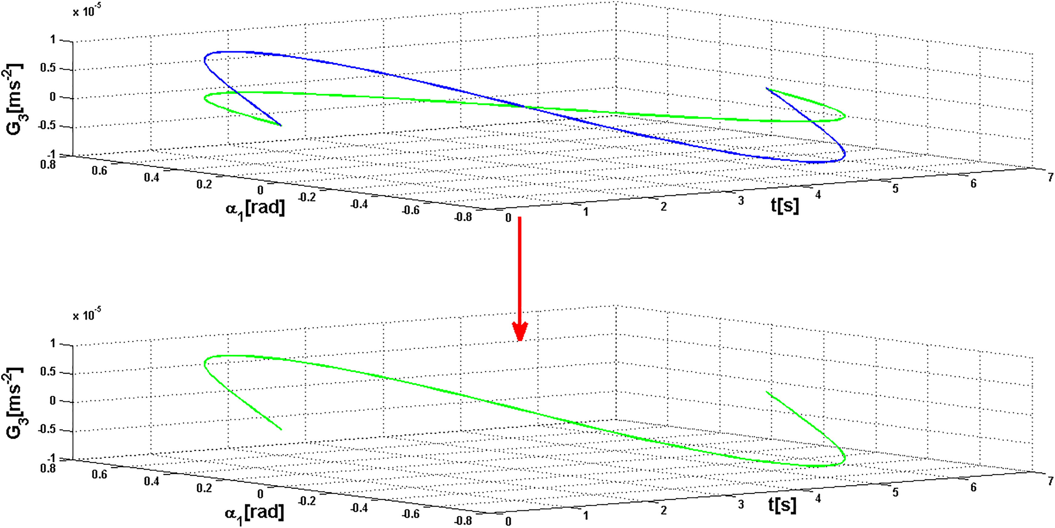
The gamma function G ₃.

In the previous figures (Figures 14 and 16), we can see that the chosen gait guaranteed maximum shift in the direction of coordinate x but also θ since the individual courses are identical.

The position change in individual directions for two-link snake will be expressed only using the dynamic phase shift and these changes of position we get using the following relations

Δ ζ^{x} = I_{D Y N}^{x} = \int [\underset{G_{1} (α_{1})}{\underset{︸}{\frac{2 (- L \cos α_{1} - R)}{J_{R} L \sin α_{1} \sin α_{1} (L \cos α_{1} + R) (J_{L} + 2 J_{R} - m_{L} - m_{R})}}} \underset{}{} (\int J_{R} \frac{L}{2} \sin α_{1} {\dot{α}}_{1} (- \frac{L}{2} \cos α_{1} - \frac{R}{2}) {\dot{α}}_{1} d t)] d t

Δ ζ^{y} = I_{D Y N}^{y} = \int [\underset{G_{2} (α_{1})}{\underset{︸}{0}} (\int J_{R} \frac{L}{2} \sin α_{1} {\dot{α}}_{1} (- \frac{L}{2} \cos α_{1} - \frac{R}{2}) {\dot{α}}_{1} d t)] d t

Δ ζ^{θ} = I_{D Y N}^{θ} = \int [\underset{G_{3} (α_{1})}{\underset{︸}{\frac{- \frac{2}{J_{R} L}}{\sin α_{1} (L \cos α_{1} + R) (J_{L} + 2 J_{R} - m_{L} - m_{R})}}} \underset{}{} (\int J_{R} \frac{L}{2} \sin α_{1} {\dot{α}}_{1} (- \frac{L}{2} \cos α_{1} - \frac{R}{2}) {\dot{α}}_{1} d t)] d t

When we want to achieve the position change expressed in the world velocity, then it is sufficient to use the reconstruction equation of movement (44) expressed in the world velocities and proceed by the same manner.

Movement simulation of two-link snake at different modes

In the previous subchapters, we processed and confirmed the situation with validity of the following theorem: If lengths of links are different and time integrals of the base variable in both directions are the same (sinusoid represents that the course of the base variable has the same frequency during whole period), then the final phase shift is different from zero.

Now we confirm the situation by simulation the movement of the two-link snake in SolidWorks where it will apply: If lengths of links are the same and time integrals of the base variable in both directions are the same, then the final phase shift is equal to zero. The gait ϕ generating lateral movement of snake in this case will have the form as in equation (45). The distance travelled by snake at lateral movement during one period is zero, while the snake deflects only from one side to other side (Figure 17).

Figure 17.

The lateral movement of snake with trajectory of mass center during some periods.

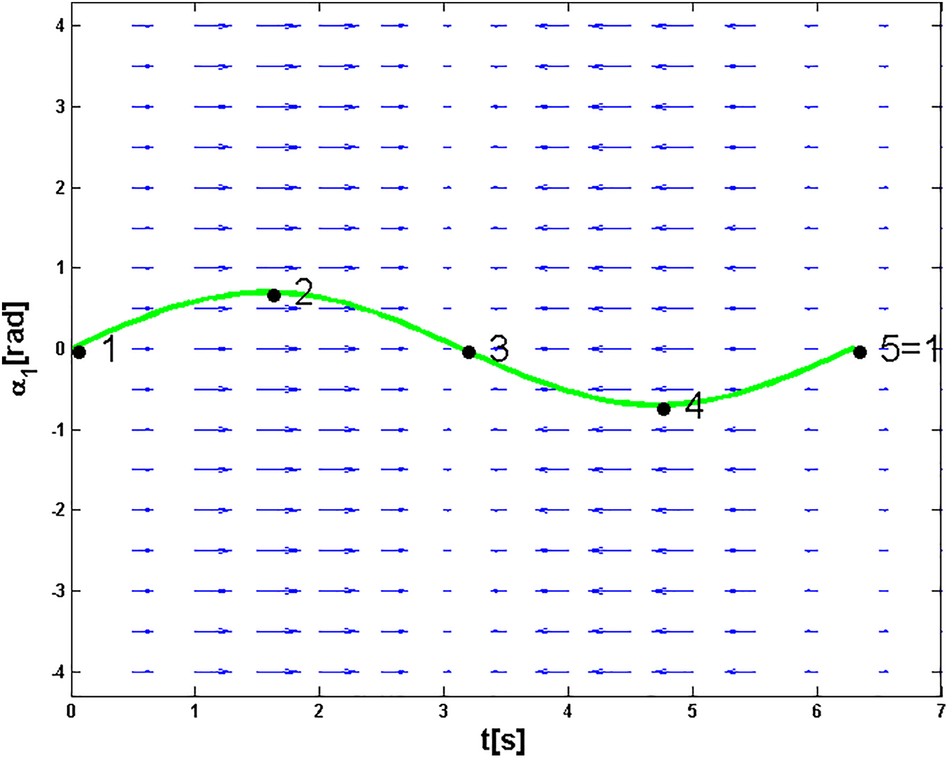
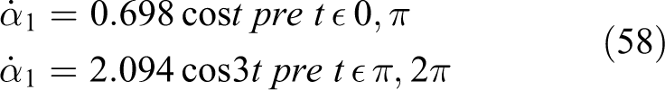
Finally, we confirm the situation: If lengths of links are the same and time integrals of the base variable in both directions are different, then the final phase shift is different from zero. The gait ϕ in this case will be (Figure 18)

\begin{matrix} α_{1} = 0.698 sin t p r e t ∊ 0, π \\ α_{1} = 0.698 sin 3 t p r e t ∊ π, 2 π \end{matrix}

Figure 18.

The rotation angle α₁ with shown half periods for lateral movement.

And then the rotation velocity is (Figure 19)

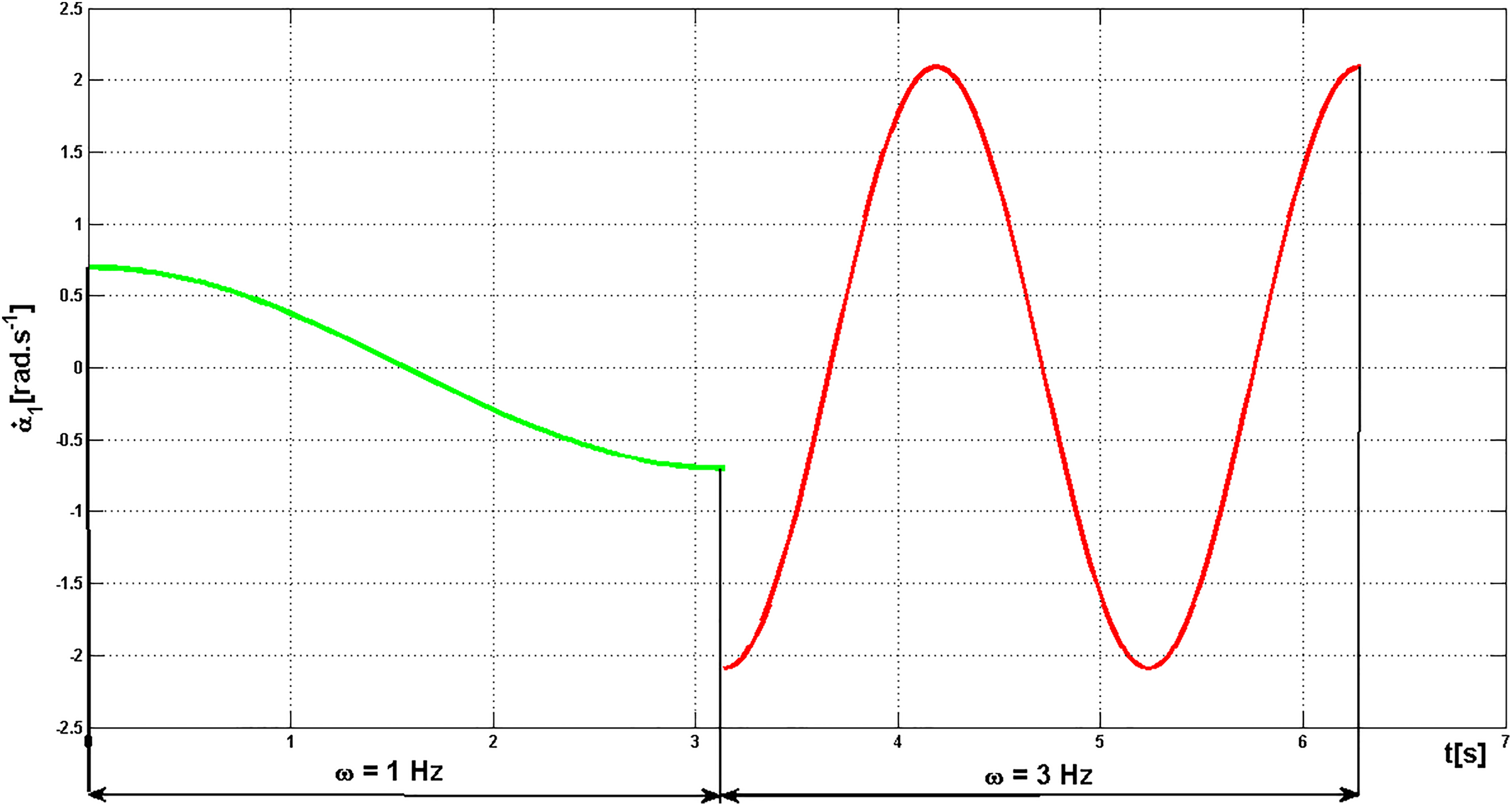
\begin{matrix} {\dot{α}}_{1} = 0.698 cos t p r e t ∊ 0, π \\ {\dot{α}}_{1} = 2.094 cos 3 t p r e t ∊ π, 2 π \end{matrix}

Figure 19.

The rotation velocity ${\dot{α}}_{1}$ with shown half periods for lateral movement.

The travelled distance at this way of movement is 17.84 mm (Figure 20).

Figure 20.

The lateral movement of snake at new form of gait.

Reduced base dynamic equation

In the previous subchapters, the case was solved where base velocities represented an ideal source of velocity, that is, at increasing load, the velocities had the constant course (Figure 21).

Figure 21.

The load characteristics of velocity source.

Now we will consider the case when the base variable changes by the influence of load. The snake will be controlled by torque and therefore we should also use the reduced base dynamic equation (8) where its solutions are base variables. Then, these base variables we substitute to reconstruction equation and get fiber velocity $\dot{g}$ or ξ. In reduced dynamic equation, we will consider the component of friction N and Coriolis forces C equal to zero

M \ddot{r} = τ (r)

Matrix of reduced mass is determined according to relation⁷

M (r) = m (r) - A {(r)}^{T} I (r) A (r)

M (r) = J_{R} - {(R sin α_{1} (m_{L} + m_{R}) - 2 J_{R} sin α_{1} (\frac{R}{2} + \frac{L}{2} cos α_{1}))}^{2} (J_{L} + J_{R}) - (m_{L} + m_{R}) {(\frac{R}{2} + \frac{L}{2} cos α_{1})}^{2} {(R (J_{L} + J_{R}) - J_{R} L cos α_{1})}^{2}

Then, the reduced dynamic equation has the form

[J_{R} - {(R sin α_{1} (m_{L} + m_{R}) - 2 J_{R} sin α_{1} (\frac{R}{2} + \frac{L}{2} cos α_{1}))}^{2} (J_{L} + J_{R}) - (m_{L} + m_{R}) {(\frac{R}{2} + \frac{L}{2} cos α_{1})}^{2} {(R (J_{L} + J_{R}) - J_{R} L cos α_{1})}^{2}] {\ddot{α}}_{1} = τ

Conclusion

The aim of the article is to show tools of geometric mechanics at creating the mathematical models. The main advantage of geometric mechanics compared with analytical mechanics (e.g. Lagrangian mechanics) is the mathematical model consisting of n − l second-order differential equations (reduced base dynamic equation) and l first-order differential equations (reconstruction equation), where at Lagrangian mechanics, we have n second-order differential equations and l first-order differential equations. The next advantage is showing of local connection by vector fields that help us at predicting movement of robotic systems. Geometric mechanics applies that the reconstruction equation does not influence the reduced base dynamic equation. We chose one type of generalized mixed locomotion systems. The two-link snake from category—mixed locomotion system was used as an example. For this system, a mathematical model consisting of the reconstruction equation and momentum equation where we considered action variable as ideal source of velocity was created. In this case, the reconstruction equation is no longer composed only of kinematic part but also of dynamic one. We simulated the movement of this system and presented height and gamma functions, where height functions are equal to zero because the base space is only one-dimensional. Finally, the reduced base dynamic equation for the case of controlling using torque was also determined.

Footnotes

Declaration of conflicting interests

The author(s) declared no potential conflicts of interest with respect to the research, authorship, and/or publication of this article.

Funding

The author(s) disclosed receipt of the following financial support for the research, authorship, and/or publication of this article: The work has been accomplished under the research projects no. VEGA 1/0872/16 “Research of synthetic and biological inspired locomotion of mechatronic systems in rugged terrain.”

References

Hatton

Choset

. Kinematic locomotion. In Book: An introduction to geometric mechanics and differential geometry, 6 December 2011, pp. 45–58.

Hatton

Choset

. Connection vector fields for underactuated systems. In: Proceedings of the 2nd biennial IEEE/RAS-EMBS international conference on biomedical robotics and biomechatronics, Scottsdale, AZ, USA, 19–22 October 2008, pp. 451–456. IEEE.

Ebetiuc

Harald

. Applying differential geometry to kinematic modeling in mobile robotics. In: WSEAS international conference on dynamical systems and control, Venice, Italy, 2–4 November 2005, pp. 106–112.

Shammas

Achmidt

Choset

. Natural gait generation techniques for multi-bodied isolated mechanical systems. In: Proceedings of the 2005 IEEE international conference on robotics and automation, Barcelona, Spain, April 2005, pp. 3664–3669. IEEE.

Karavaev

Kilin

. The dynamics and control of a spherical robot with an internal omniwheel platform. Regul Chaotic Dyn 2015; 20(2): 134–152.

Lipták

Gmiterko

Kelemen

. The process of gait generation for snake-like robot with nonholonomic constraints. Appl Mech Mater 2015; 816: 240–247.

Shammas

. Generalized motion planning for underactuated mechanical systems. Thesis, Carnegie Mellon University Pittsburgh, Pennsylvania, 20 3 2006.

Hatton

Choset

. Optimizing coordinate choice for locomoting systems. In: IEEE international conference on robotics and automation anchorage convention district, Anchorage, Alaska, USA, 3–8 May 2010, pp. 4493–4498. IEEE.

Bloch

Baillieul

Crouch

. Nonholonomic mechanics and control. USA: Department of Mathematics, University of Michigan, 2003.

10.

Karavaev

Kilin

. Nonholonomic dynamics and control of a spherical robot with an internal omniwheel platform: theory and experiments. Proc Steklov Inst Math 2016; 295(1): 158–167.

11.

Koniar

Hargas

Simonova

. Virtual instrumentation for visual inspection in mechatronic applications. In: 6th conference on modelling of mechanical and mechatronic systems (MMaMS), Vysoke Tatry, Slovakia, 25–27 November 2014. Elsevier.

12.

Trebuňa

Virgala

Pástor

. An inspection of pipe by snake robot. Int J Adv Robotic Syst 2016; 13(5): 1–12.

13.

Nirody

Scott

. The mechanics of slithering locomotion. Proc Natl Acad Sci USA 2009; 106: 10081–10085.

14.

Shapere

Wilczek

. Geometry of self-propulsion at low Reynolds number. J Fluid Mech 1989; 198: 557–585.

15.

Murray

Sastry

. Nonholonomic motion planning: steering using sinusoids. In: IEEE Transactions on Automatic Control, vol. 38(5), May 1993, pp. 700–716. IEEE.

16.

Kelly

Murray

. Geometric phases and robotic locomotion. In: Journal Robotic System, CDS Technical Report, vol. 12(6), 1995, pp. 417–431.

17.

Ostrowski

JP.

The mechanics and control of undulatory robotic locomotion. The dissertation thesis, California Institute of Technology Pasadena, 19 9 1995.

18.

Ostrowski

. Computing reduced equations for robotic systems with constraints and symmetries. In: IEEE Transactions on Robotics and Automation, vol. 15(1), February 1999, pp. 111–123.

Modeling and control of two-link snake

Abstract

Keywords

Introduction

Generalized mixed mechanical locomotion system

Mixed mechanical locomotion system

Nonholonomic constraints and Lagrangian

Reconstruction equation

Momentum evolution equation

Representation of local connection using vector fields

Height and gamma functions of two-link snake

Movement simulation of two-link snake at different modes

Reduced base dynamic equation

Conclusion

Footnotes

Declaration of conflicting interests

Funding

References