Sage Journals: Discover world-class research

Abstract

This article deals with the design of an optimal tracking controller for a wheeled mobile robot. The tracking control can be performed to track either a given or a planned trajectory. In our study, an improved linear quadratic tracker is adopted to track a path planned using an improved reactive approach that combines the dynamic window with the fuzzy logic to make the robot movement toward the target faster, smoother, and safer whatever the complexity of the environment. The fuzzy logic is used to dynamically adjust the weights of the terms included in the dynamic window objective function according to different environmental scenarios. Simulation results of the path planning and the tracking control prove that the proposed approaches are significantly superior to the conventional ones.

Keywords

Mobile robot dynamic window approach fuzzy control optimal tracking control

Introduction

In recent years, a lot of researches have been published about the path planning and the tracking control due to their importance in the field of mobile robotics. The majority of the authors have dealt with these two tasks separately; in this article, we try to achieve the continuity between them.

There have been many path planning techniques proposed in the literature; we have chosen the reactive method known as the dynamic window approach (DWA)¹ because it takes the mobile robot dynamics into account.

The DWA was proposed by Fox in 1996 to be used in high-speed navigation by searching for control commands directly in the space of velocities. Brock and Khatib² extended the original DW to a global DWA by using connectivity information about the free space to avoid the local minima. Arras et al.³ reduced the DW to speed up the translational velocity selection. Philippsen and Siegwart⁴ combined the DW, the elastic band, and NF1 to guarantee the convergence toward the target.

The control commands in the DWA are selected by maximizing an objective function, which is a weighted sum of three terms, and their main role is driving the robot fast and safe to the goal; however, this is not always guaranteed, due to the problem of choosing the appropriate weights. Several studies have been done to modify the objective function such as combining the DW with a particle filter to optimize the objective function,⁵ employing fuzzy logic to change the velocity according to the obstacle density,⁶ extending the classic DWA to a global DWA-based navigation scheme using model predictive control without an objective function,⁷ and recently using a two-stage fuzzy-DWA: the first one to determine the heading angle and the second one to compute the target wheel velocities of the robot.⁸ None of the mentioned extensions has solved the problem of finding suitable weights for the objective function.

The path tracking control is the process of determining speed and steering settings at each time step in order to make the robot follow a certain path. Various control strategies have been proposed over the years to handle this task, like the predictive control,^9,10 the backstepping control,^11,12 the adaptive control,^13,14 and the fuzzy adaptive control.¹⁵

In this article, the DWA is improved by using a fuzzy controller to dynamically adjust the weights of the objective function seeking for a fast and safe movement of the mobile robot. For the tracking control, a discrete linear quadratic tracker (LQT)^16,17 with an additional control law is employed to ensure fast convergence of the mobile robot to the desired path and to maintain its stability along this path.

The article is organized as follows: The second section presents a brief description of the DWA with its disadvantages and our proposed approach. In the third section, a discrete LQT is designed. The fourth section discusses the simulation results, and the final section concludes the article.

Dynamic window approach

The DWA is a reactive path planning and obstacle avoidance technique designed to achieve high-speed navigation using the translational velocity (v) and the rotational velocity (w). These velocities must be optimal, safe, and selected from the velocity search space; therefore, the task of finding them is formulated as an optimization problem, which is feasible only for a discrete set of velocities bounded by v _max and w _max. The unsafe velocities are considered as nonadmissible and discarded from further calculations; in other words, we can say that the search space is reduced to three subspaces: the possible velocities V_d , the admissible velocities V_a , and the restricted initial velocities V_s . The intersection of the three subspaces gives the resulting search space V_r

V_{r} = V_{s} \cap V_{a} \cap V_{d}

From V_r , the optimal velocities will be selected by maximizing the following objective function

G (v, w) = α \cdot head (v, w) + β \cdot dist (v, w) + γ \cdot vel (v, w)

where head is the function that keeps the robot going toward the goal location, dist is the distance to the closest obstacle; it saves the robot from collision, and vel is the forward velocity that makes the robot move fast. α, β, and γ are weighting factors used to control the influence of the terms included in the objective function on the behavior of the robot.

Drawbacks of the dynamic window

As in other reactive approaches,¹⁸ during the process of path planning using the DWA, we have found that the robot can reach the goal position easily and safely in several environments with less number of obstacles; unfortunately, this is not the case if the environment is crowded.

We have done a lot of simulations by changing the weights α, β, and γ in order to get a universal set or a set that suits for many complex environments, which was impossible because the robot performed this kind of behaviors multiple times:

Unable to move around or pass the first obstacle

Figure 1 shows that if we choose a high value for α, a low value for β, and whatever the value of γ, the robot will always be stopped by the first obstacle in its path.

Incapable of going across the narrow space between obstacles¹⁸

Figure 1.

The robot can’t avoid the first obstacle.

Figure 2 shows that if we choose a low value for α and a high value for β, the robot will perform a long path to the goal.

Going to a free space or passing the target

Figure 2.

The robot can’t cross the narrow spaces.

Figure 3 shows that if we choose a high value for β and γ, the robot will cross the goal.

Reaching the target without performing an optimal path¹⁸

Figure 3.

The robot passes the target position.

Figure 4 shows that if we choose equal or close values for α, β, and γ, then after several simulations using different sets, the robot can make a short path to the goal compared to Figure 2; however, it is not the shortest.

Figure 4.

The robot performs a short path.

In this section, like the authors in the original DW and its extensions, we have used random sets of weights. In the next section, we are going to use a fuzzy controller to adjust those weights in real time.

Real-time weights adjustment

The objective function is responsible for the DWA’s good or bad performance and the weights α, β, and γ are the key for that; therefore, to change the performance, we have to change the weights. In our work, these weights are adjusted dynamically according to the current environmental scenario using fuzzy logic, which is highly recommended in this kind of issues.

The fuzzy controller has three inputs and three outputs. The inputs are the current distance (dist) between the robot and each of the detected obstacles on the path, the forward velocity (vel), and the target heading angle (head). The outputs are the weights α, β, and γ. The distance range is [0, 15 m], divided into three subranges: close, medium, and far; the velocity domain contains three subdomains: slow, normal, and fast; the heading angle range is [0, 180°], divided into three fields: little, more and lots; the weights range is [0, 1] divided into three subdomains: low, medium and high. The definitions of the membership functions are shown in Figure 5(a) and (b).

Figure 5.

(a) Membership functions of the fuzzy inputs, (b) Membership functions of the fuzzy outputs, (c) Flowchart of the fuzzy-DWA. DWA: dynamic window approach.

Figure 5(c) shows the flowchart of the proposed fuzzy-DWA. Before starting the path planning process, we must have map information like target and obstacles coordinates, and we have to initialize the weights to be used in the first iteration, then the fuzzy controller will adjust them dynamically until the robot reaches the target.

Table 1 summarizes the fuzzy rules used in the controller design based on logic arguments like

– If the robot is far away from an obstacle, α and γ should be high and β should be low.

– If the robot is approaching an obstacle, we should increase β and reduce α and γ.

– If the robot is passing an obstacle, we must reduce β and increase α and γ.

– If the robot is approaching the target, we have to decrease β and γ and increase α.

Table 1.

The sets of rules used in the fuzzy controller.

Rule number	Linguistic inputs			Linguistic outputs
Rule number	Dist	Vel	Head	α	β	γ
1	Close	Slow	Little	Low	High	Low
2	Close	Normal	More	Low	High	Low
3	Close	Fast	Lots	Low	High	Low
4	Medium	Slow	Little	Medium	Low	Medium
5	Medium	Normal	More	Medium	Low	Medium
6	Medium	Fast	Lots	Low	Medium	Medium
7	Far	Slow	Little	High	Low	High
8	Far	Normal	More	High	Low	High
9	Far	Fast	Lots	High	Low	High

Dist: distance; Vel: velocity; Head: heading angle.

Tracking control

The main purpose of the tracking control is making the robot follow a desired path, in our case this path is planned using fuzzy-DWA.

Kinematic model of the mobile robot

The state space model of the mobile robot in Figure 6 is given by

{\begin{cases} \dot{x} = v cos θ \\ \dot{y} = v sin θ \\ \dot{θ} = w \end{cases}

Figure 6.

The model of the mobile robot.

And can be written in a compact form as

\dot{x} = f (x, u)

where ${[x y θ]}^{T}$ describes the position and the orientation of the robot and ${[u = v w]}^{T}$ represents the control input.

The discrete time state space model at sample rate T_s is given as follows

{\begin{cases} x (k + 1) = x (k) + T_{s} u_{1} (k) cos θ \\ y (k + 1) = y (k) + T_{s} u_{1} (k) sin θ \\ θ (k + 1) = θ (k) + T_{s} u_{2} (k) \end{cases}

From equation (5), it can be seen that the equations representation can be formulated in linear state space form

x (k + 1) = A x (k) + B u (k)

where $A = [\begin{matrix} 1 & 0 & 0 \\ 0 & 1 & 0 \\ 0 & 0 & 1 \end{matrix}] and B = [\begin{matrix} \begin{matrix} T_{s} cos θ \\ T_{s} sin θ \\ 0 \end{matrix} & \begin{matrix} 0 \\ 0 \\ T_{s} \end{matrix} \end{matrix}]$

Linear quadratic tracker

The LQT generates optimal control inputs that make the robot track the desired path with the minimum tracking error. To obtain these optimal control inputs, a performance index should be minimized.

Equation (7) represents the discrete time performance index to be minimized^16,17

\begin{array}{l} J = \frac{1}{2} {[C x (k_{f}) - r (k_{f})]}^{T} F [C x (k_{f}) - r (k_{f})] \\ + \frac{1}{2} \sum_{k = k_{0}}^{k_{f} - 1} {{[C x (k) - r (k)]}^{T} Q [C x (k) - r (k)] + u^{T} (k) R u (k)} \end{array}

where x(k) and u(k) are the state and the control vectors at time step k, respectively. C is the discrete time output matrix. F ≥ 0, Q ≥ 0, and R > 0 are diagonal weighting matrices that penalize the final state, the state, and the control inputs, respectively. r(k) represents the desired state vector which contains the coordinates of the reference trajectory at each time step.

To solve the minimization problem in equation (7), the Hamiltonian is defined as

\begin{array}{l} H (x (k), u (k), λ (k + 1)) = \frac{1}{2} \sum_{k = k_{0}}^{k_{f} - 1} {{[C x (k) - r (k)]}^{T} Q [C x (k) - r (k)] \\ + u^{T} (k) R u (k)} + λ^{T} (k + 1) [A x (k) + B u (k)] \end{array}

where λ is the Lagrange multiplier that is derived from the Hamiltonian as shown in equation (9)

λ (k) = \frac{\partial H}{\partial x (k)}

λ (k) = A^{T} λ (k + 1) + V x (k) - W r (k)

with $V = C^{T} Q C and W = C^{T} Q$ .

Equation (9) is also called the costate, and its final state is given by

λ (k_{f}) = C^{T} F C x (k_{f}) - C^{T} F r (k_{f})

By deriving the Hamiltonian with respect to the control input, we get the open loop optimal control law as

\frac{\partial H}{\partial u (k)} = 0

u (k) = - R^{- 1} B^{T} λ (k + 1)

By substituting equation (11) in equation (6), we obtain the state space in the following form

x (k + 1) = A x (k) - B R^{- 1} B^{T} λ (k + 1)

The combination of equations (12) and (9) yields the so-called homogeneous Hamiltonian system

[\begin{array}{l} x (k + 1) \\ λ (k) \end{array}] = [\begin{matrix} \begin{array}{l} A \\ V \end{array} & \begin{array}{l} - E \\ A^{T} \end{array} \end{matrix}] [\begin{array}{l} x (k) \\ λ (k + 1) \end{array}] + [\begin{array}{l} 0 \\ - W \end{array}] r (k)

where $E = B R^{- 1} B^{T}$ .

Due to the forcing term $C^{T} Q r (k)$ in equations (9) and (10), the optimal control is no longer a linear state feedback; however, it can be expressed as a combination of a linear state feedback plus a term depending on r(k).¹⁶

According to equation (10), we assume that for all k < N, we can write

λ (k) = P (k) x (k) - g (k)

To validate the assumption in equation (14), consistent equations for P(k) and g(k) must be found. To do so, we use equation (14) in the state equation portion of equation (13) and after a few calculations,¹⁶ we get the following equations

P (k) = A^{T} P (k + 1) {[I + E P (k + 1)]}^{- 1} A + V

g (k) = {A^{T} - A^{T} P (k + 1) {[I + E P (k + 1)]}^{- 1} E} g (k + 1) + W r (k)

By comparing equations (14) and (10), the boundary conditions for P(k) and g(k) are defined by

P (k_{f}) = C^{T} F C

g (k_{f}) = C^{T} F r (k)

Solving backward in time both of equation (15) and equation (16) using the boundary conditions in equation (17) and equation (18), respectively, leads to the time varying gains L(k) in equation (19) and L_g (k) in equation (20), which are used to formulate the closed loop optimal control law in equation (21)

L (k) = {[R + B^{T} P (k + 1) B]}^{- 1} B^{T} P (k + 1) A

L_{g} (k) = {[R + B^{T} P (k + 1) B]}^{- 1} B^{T}

u (k) = - L (k) x (k) + L_{g} (k) g (k + 1)

Consequently, the resulting optimal state is expressed as follows

x (k + 1) = [A - B L (k)] x (k) + B L_{g} (k) g (k + 1)

In this article, to ensure a fast transition of the robot from any initial position toward the reference trajectory, the performance index is extended to the following form

\begin{array}{l} J = \frac{1}{2} {[C x (k_{f}) - r (k_{f})]}^{T} F [C x (k_{f}) - r (k_{f})] \\ + \frac{1}{2} \sum_{k = k_{0}}^{k_{f} - 1} {{[C x (k) - r (k)]}^{T} Q [C x (k) - r (k)] \\ + {[u (k) - u_{r} (k)]}^{T} R [u (k) - u_{r} (k)]} \end{array}

where u_r is the control input that makes the robot reaches the desired path quickly and maintains its stability along this path, which can be calculated as follows

A r (k) + B u_{r} (k) = 0

u_{r} (k) = - B^{- 1} A r (k)

The optimal control law in this case is expressed as

u (k) - u_{r} (k) = - L (k) [x (k) - r (k)] + L_{g} (k) g (k + 1)

u (k) = - L (k) x (k) + L_{g} (k) g (k + 1) + [L (k) - B^{- 1} A] r (k)

The proposed control strategy can be seen in Figure 7.

Figure 7.

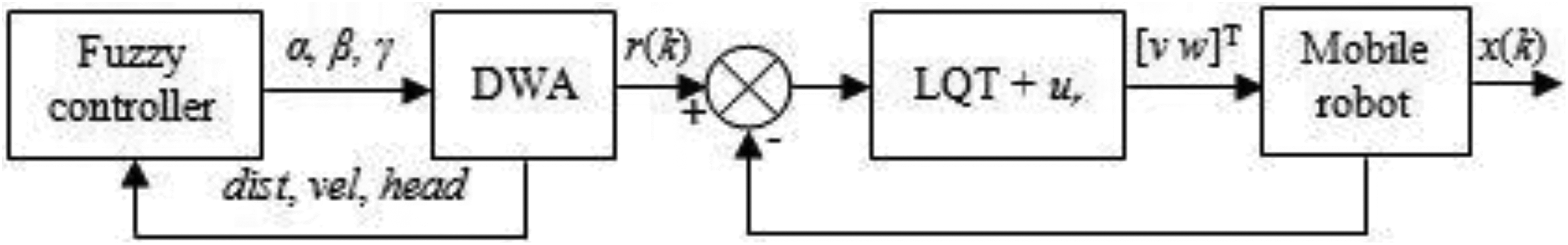
Block diagram of the path planner and the optimal tracking controller.

Simulation results

The DWA and the fuzzy-DWA, the LQT and the LQT + u_r algorithms are implemented and compared in Matlab. The robot has a circular shape with a radius of 0.15 m and moves in two different maps of the size 15 m × 15 m and 25 m × 25 m. The maximum translational and rotational velocities are 1 m/s and 90°/s, respectively. At each iteration, the weights of the objective function must satisfy this condition: α + β + γ ≤ 1. The sample rate T_s is 0.1 s. The performance index parameters are assumed as follows: F = I ₃, Q = 10 × I ₃, and R = I ₃. The lemniscate shape trajectory is given by these equations: x(t) = 1.1 + 0.7 sin(2t/30) and y(t) = 0.9 + 0.7 sin(4t/30).

Path planning results

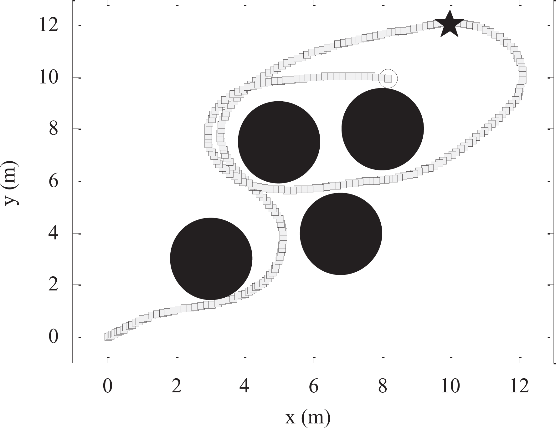
By comparing Figure 8(a) with Figures 1 to 4, it is obvious that the proposed fuzzy-DWA has improved the performance of the mobile robot by making it reach the goal safely with the shortest path possible. In Figure 8(b) to (d), we can see how the weights change according to the environment situation.

Figure 8.

(a) Optimal path generated by the fuzzy-DWA, (b) corresponding α values, (c) corresponding β values, and (d) corresponding γ values. DWA: dynamic window approach.

Figure 9 as well shows the efficiency of the proposed approach in driving the robot toward the target through a complex environment, and it displays the weights adjustment during the path planning process.

Figure 9.

(a) Optimal path generated by the fuzzy-DWA, (b) corresponding α values, (c) corresponding β values, and (d) corresponding γ values.

In Figure 10(a), the robot can reach the goal from several starting positions, and in Figure 10(b), it is able to travel from the same position to different targets, which confirms the robustness of our approach.

Figure 10.

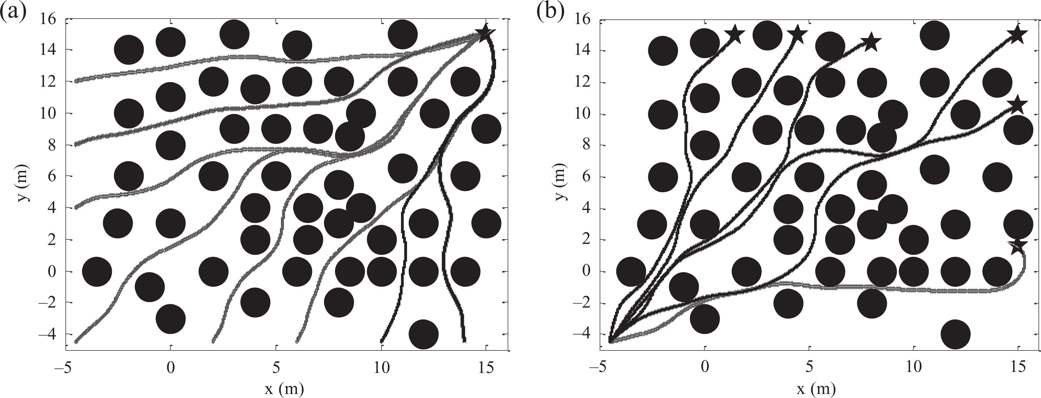
Fuzzy-DWA path planning (a) from several positions and (b) to different goals. DWA: dynamic window approach.

Tracking control results

Figure 11(a) and (b) shows a comparison between the trajectories obtained by applying the conventional LQT controller and our LQT + u_r controller. The tracking errors are shown in Figure 12(a) and (b). According to Figure 11, both controllers perform a good tracking of the desired trajectories; however, the LQT + u_r shows better accuracy in the tracking performance which can be seen in Figure 12, as a fast convergence of the tracking errors and more stability along the trajectories.

Figure 11.

(a) Tracking a planned trajectory and (b) tracking a given trajectory.

Figure 12.

(a) Tracking errors of the planned trajectory and (b) tracking errors of the given trajectory.

Conclusion

In this article, a fuzzy controller was used to dynamically adjust the weights of the DW objective function, and a control law was added to the LQT to improve the tracking performances. Simulation results of the path planning prove that the proposed fuzzy-DWA is significantly superior to the original DW, especially in cramped environments with numerous obstacles. The optimal tracking control results indicate that the proposed LQT + u_r controller achieves better tracking performances.

It is clear that the results achieved in this article prove the potential of the fuzzy-DWA in solving the path planning problem, and the effectiveness of the LQT in tracking different trajectories. Future goals are to perform the path planning in dynamic environment and to focus on the experimental validation of the proposed algorithm.

Footnotes

Declaration of conflicting interests

The author(s) declared no potential conflicts of interest with respect to the research, authorship, and/or publication of this article.

Funding

The author(s) received no financial support for the research, authorship, and/or publication of this article.

ORCID iD

Khaled Akka

References

Fox

Burgard

Thrun

. Controlling synchro-drive robots with the dynamic window approach to collision avoidance: Proceedings of the 1996 IEEE/RSJ international conference on intel ligent robots and systems, Osaka, Japan, 8 November 1996, pp. 1280–1287. IEEE.

Brock

Khatib

. High-speed navigation using the global dynamic window approach. In: Proceedings of the 1999 IEEE international conference on robotics and automation, Detroit, MI, USA, 10–15 May 1999, pp. 341–346. IEEE.

Arras

Persson

Tomatis

. Real-time obstacle avoidance for polygonal robots with a reduced dynamic window. In: Proceedings of the 2002 IEEE international conference on robotics and automation, Washington, DC, USA, 11–15 May 2002, pp. 3050–3055. IEEE.

Philippsen

Siegwart

. Smooth and efficient obstacle avoidance for a tour guide robot. In: Proceedings of the 2003 IEEE international conference on robotics and automation, Taipei, Taiwan, 14–19 September 2003, pp. 446–451.

Schröter

Höchemer

Gross

. A particle filter for the dynamic window approach to mobile robot control. In: Proceedings of the 2007 international scientific colloquium (IWK), vol. 1, Ilmenau, Germany, 2007, pp. 425–430.

Choi

Kim

. A modified dynamic window approach in crowded indoor environment for intelligent transport robot. In: Proceedings of the 2012 12th international conference on control, automation and systems, JeJu Island, South Korea, 17–21 October 2012, pp. 1007–1009. ICROS.

Kiss

Tevesz

. Advanced dynamic window based navigation approach using model predictive control. In: Proceedings of the 2012 17th international conference on methods and models in automation and robotics, Miedzyzdrojie, Poland, 27–30 August 2012, pp. 149–153. IEEE.

Chand

Fuzzy reactive control for wheeled mobile robots. In: Proceedings of the 2015 6th international conference on automation, robotics and applications, Queenstown, New Zealand, 17–19 February 2015, pp. 167–172. IEEE.

Klančar

Škrjanc

. Predictive trajectory tracking control for mobile robots. In: EPE-PEMC, Portoroz, Slovenia, 30 August-1 September 2006, pp. 373–378. IEEE.

10.

Klančar

Škrjanc

. Tracking-error model-based predictive control for mobile robots in real time. Rob Autonom Syst 2007; 55: 460–469.

11.

Umesh

Nagarajan

. Backstepping based trajectory tracking control of a four wheeled mobile robot. Int J Adv Rob Syst 2008; 5(4): 403–410.

12.

Chwa

. Tracking control of differential-drive wheeled mobile robots using a backstepping-like feedback linearization. IEEE Trans Syst Man Cybern A Syst Hum 2010; 40(6): 1285–1295.

13.

Huang

. Adaptive tracking control of high-order non-holonomic mobile robot systems. IET Control Theory Appl 2009; 3(6): 681–690.

14.

Park

Yoo

Park

. Adaptive output-feedback control for trajectory tracking of electrically driven non-holonomic mobile robots. IET Control Theory Appl 2011; 5(6): 830–838.

15.

Chwa

. Fuzzy adaptive tracking control of wheeled mobile robots with state-dependent kinematic and dynamic disturbances. IEEE Transaction Fuzzy Syst 2012; 20(3): 587–593.

16.

Lewis

Syrmos

. Optimal control. 2nd ed. New York: John Wiley & Sons, 1995.

17.

Hashemi

Ghaffari Jadidi

. Model-based PI–fuzzy control of four-wheeled omni-directional mobile robots. Rob Auton Syst 2011; 59: 930–942.

18.

Savkin

Hoy

. Reactive and shortest path navigation of a wheeled mobile robot in cluttered environments. Robotica 2013; 31(2): 323–330.