Sage Journals: Discover world-class research

Abstract

The Five-hundred-meter Aperture Spherical radio Telescope is the world’s largest single-dish radio telescope and is located in the southwest of China. The cable-driven parallel robot and A-B rotator of the feed support system in Five-hundred-meter Aperture Spherical radio Telescope are designed to realize the theoretical position and attitude of the receiver. The feed support system is a pose-redundant and rigid–flexible coupling system; thus, the method of pose distribution between the A-B rotator and the cable-driven parallel robot impacts on the cable tension distribution and stiffness of the feed support system, which are crucial to the feed support system stability. The main purpose of this study is to examine the pose optimal distribution method for the feed support system. First, a mechanical model of the feed support system, which considers the time-varying barycenter of the feed cabin and the back-illuminated strategy of the receiver, is established. Then, a pose distribution method that ensures the position and attitude accuracy of the receiver is proposed for the feed support system. Considering the performance indices of the variance of cable tensions and the stiffness of the cable-driven parallel robot, an optimization of the rotation angles of the A-B rotator with multiple objectives is implemented using a genetic algorithm. Finally, simulations are conducted to demonstrate the effectiveness of the proposed method compared with others. Results show that the proposed approach not only ensures the attitude accuracy of the receiver but also maintains the lower variance of cable tensions and higher stiffness of the feed support system.

Keywords

Pose distribution multi-objective time-varying barycenter stiffness FAST

Introduction

The Five-hundred-meter Aperture Spherical radio Telescope (FAST) is the largest single-dish radio telescope in the world and is located in Guizhou province in the southwest of China.^1,2 It primarily consists of a feed support system (FSS), an active reflector system, and a receiver system.^3,4 A photograph of FAST is shown in Figure 1.

Figure 1.

Photograph of FAST. FAST: Five-hundred-meter Aperture Spherical radio Telescope.

The FSS is composed of a six-cable-driven parallel robot (CDPR) and a feed cabin.^5
–7 As shown in Figure 2, the feed cabin contains three mechanisms: a star frame, A-B rotator, and rigid Stewart manipulator. The star frame acts as the active platform of the CDPR. The CDPR and A-B rotator are designed to realize the theoretical pose of the receiver. The rigid Stewart manipulator is designed to compensate the position and attitude deviation of the receiver which are caused by the wind vibration and other external disturbances.⁸

Figure 2.

Diagram of the feed cabin.

According to the special structure of the FSS, several technical issues need specific consideration. First, the rotation of the A-B rotator and the adjustment of the rigid Stewart manipulator change the barycenter of the feed cabin, which should be considered in the FSS mechanical model.⁵ Second, the back-illuminated strategy of the receiver should be added to the FSS model because the illumination area of the receiver may transcend the region of the active reflector. Third, owing to the redundancy of the attitude distribution between the A-B rotator and the CDPR, and because the A-B rotator cannot compensate the rotation of three degrees of freedom (3-DOFs), the receiver pose should be properly allocated to the CDPR and A-B rotator to satisfy the requirement of FSS stability and accuracy.

The CDPR mechanical model has been widely studied, including by the researchers at Xidian University,^9,10 Tsinghua University,^11,12 and the National Astronomical Observatories, Chinese Academy of Sciences.^13,14 The model of the time-varying barycenter was developed by Chai et al.¹⁵ However, none of the above studies considered the back-illuminated strategy of the receiver. Li et al.¹⁶ allocated the pose of receiver to the CDPR and the A-B rotator using the principle of minimum variance of cable tensions. Tang et al.⁸ determined that the cable tensions are evenly distributed when the ratio of tilt angles of the CDPR and A-B rotator is 3:5. Yao et al.¹⁷ presented a pose planning method for the FSS. However, these pose distribution studies do not consider the FSS stiffness.

Owing to the long-span flexibility cable structure, the FSS is sensitive to external disturbance.¹⁸ Stiffness can characterize the ability of FSS to resist external disturbances. The FSS stiffness is far less than that of the rigid-link parallel robot. Li¹⁹ derived the FSS stiffness by calculating the Jacobian matrix derivatives. Raid²⁰ derived the tangential stiffness of a two-node catenary cable element. Accordingly, Zi²¹ derived the static stiffness matrix of the CDPR; however, the effect of the time-varying barycenter and the rotation matrix differential from the cable coordinate system to the global coordinate system were ignored. In this study, the derivation of FSS stiffness is intended to resolve these deficiencies.

The remainder of this article is organized as follows. In the “FSS description and modeling” section, the description and modeling of the FSS are provided. A pose distribution method, which ensures the receiver pose accuracy, is designed for the FSS in the “FSS pose distribution algorithm” section. In the “Multi-objective optimization for pose distribution” section, the multi-objective optimization for pose distribution is illustrated. Numerical simulation and discussion are presented in the section that is named accordingly. Finally, in the last section, conclusions and future work are provided.

FSS description and modeling

Description of the FSS

As shown is Figure 2, the FSS contains a six-CDPR and a feed cabin. The rigid Stewart manipulator is assembled in the feed cabin, and the receiver is mounted on the active platform of the Stewart manipulator. The target of the FSS is to control the receiver to operate stably and accurately. The receiver workspace is schematically illustrated in Figure 3. During the observation, the receiver moves on the focal surface, which is a virtual surface formed by different focal points of the active reflector. Angle α is the azimuth angle of the receiver in the global coordinate system {O_G-X_GY_GZ_G }. Angle θ ₀ is the theoretical target tilt angle of the receiver. It is defined as the acute angle between the Z_G-axis and the line of point O_G and the receiver. Angle θ is the actual tilt angle of the receiver. It is defined as the angle between the Z_G-axis and the center normal vector of the active platform. The actual tilt angle of the receiver is obtained through the cooperation of the CDPR and A-B rotator.

Figure 3.

Schematic diagram of the receiver workspace.

CDPR static equilibrium equation

Figure 4 depicts the FSS-related coordinate systems. All coordinate systems comply with the right-hand rule. The six support towers are uniformly distributed on the circumference having a 600-m diameter. The related coordinate systems are defined as follows.

Figure 4.

FSS-related coordinate systems. FSS: feed support system.

Let {G} (O_G-X_GY_GZ_G ) be the global coordinate system. It is attached to the spherical center of the active reflector; the x-axis points to geographical east direction, and the z-axis points in the direction opposite to the force of gravity.

Let {C} (O_C-X_CY_CZ_C ) be the star-frame coordinate system. It is attached to the geometric center of the plane formed by six anchor nodes (B ₁ to B ₆). The x-axis crosses the midpoint of B ₁ B ₆, and the z-axis is perpendicular to the star frame.

Let {AB} (O_AB-X_ABY_ABZ_AB ) be the A-B rotator coordinate system. It is attached to the intersection of the A-axis and B-axis with the x-axis along the A-axis, and the y-axis along the B-axis.

Let {B} (O_B-X_BY_BZ_B ) be the base platform coordinate system. It is attached to the geometric center of the plane formed by six Hooke hinge joints in the base platform. Its three axes are always parallel to the three axes of {AB} and with the same pointing direction.

Let {P} (O_P-X_PY_PZ_P ) be the active platform coordinate system. It is attached to the geometric center of the plane formed by six spherical joints of the active platform. The y-axis points to the midpoint of the line connected by spherical joint 2 and spherical joint 3. The z-axis is perpendicular to the active platform.

When the feed cabin is located on the center point of the focal surface, and the FSS is on the initial pose, the three axes of each coordinate system are, respectively, parallel to each other and with the same pointing direction.

In the following, vectors and matrices are denoted in bold. The right subscripts of notations imply their physical meanings, while the left superscripts represent the coordinate systems under which they are described.

According to the demand of the astronomical observation, the FSS moves so slowly that it can be considered static. The CDPR static equilibrium equation can be derived as

[\begin{array}{l} \sum_{i = 1}^{6} {}^{G}T_{B i} + G \\ \sum_{i = 1}^{6} ({}^{G}R_{C} {}^{C}B_{i}) \times {}^{G}T_{B i} + M_{G} \end{array}] = 0

where ^G T _Bi is the tension of the ith cable acting on the feed cabin, ^C B _i is the position of the ith anchor node with respect to {C}, and G = [0,0, m_G·g ] ^T is the gravity vector of the feed cabin. Additionally, M _G is the gravity moment vector of the feed cabin, which is expressed as

M_{G} = ({}^{G}R_{C} {}^{C}P_{G}) \times G

where ^C P _G represents the time-varying barycenter of the feed cabin. The derivations of ^G T _Bi , ^G R _C , and ^G P _C are given in the following sections.

Suspension cable modeling

In the presented model, the cable weight is non-negligible²² and each cable is considered an inextensible catenary. The tension diagram of a single cable is shown in Figure 5. Let { T_i } (o_i-x_iz_i ) be the ith cable coordinate system, which is attached to the ith anchor node with the z-axis in the direction opposite to the force of gravity and with the x-axis horizontally pointing to the ith support tower.

Figure 5.

Tension diagram of a single cable.

With respect to {T_i }, the catenary equation of a single cable can be written as⁹

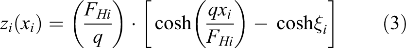
z_{i} (x_{i}) = (\frac{F_{H i}}{q}) \cdot [cosh (\frac{q x_{i}}{F_{H i}}) - cosh ξ_{i}]

where q is the linear density of the cables, F_Hi is the horizontal component of tension T _Bi , and ξ_i is an intermediate variable which is given by

ξ_{i} = arcsin h_{i} \cdot (\frac{q h_{i}}{(2 F_{H i} sinh η_{i})} - η_{i})

η_{i} = \frac{q l_{i}}{(2 F_{H i})}

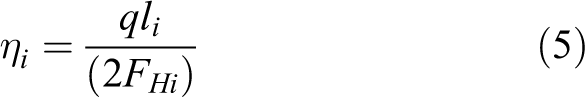
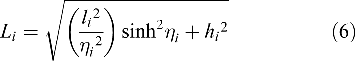
Here, h_i represents the height of the ith cable and l_i denotes the horizontal span of the ith cable. According to the expression d ² L_i = d ² x_i + d ² z_i , the cable length can be expressed as

L_{i} = \sqrt{(\frac{l_{i}^{2}}{η_{i}^{2}}) {sinh}^{2} η_{i} + h_{i}^{2}}

Let ^G T _Ai represents the tension of the ith cable that acts on point A_i . The vertical component of tensions ^G T _Bi and ^G T _Ai can be derived as⁹

F_{i B_V} = (\frac{q}{2}) \cdot (\frac{h_{i} \cdot cosh η_{i}}{sinh η_{i}})

F_{i A_V} = F_{i B_V} + q L_{i}

The cable tensions at points A_i and B_i can be expressed as

{}^{G}T_{B i} = F_{H i} {}^{G}a_{i} + F_{i B_V} {}^{G}z_{i}

{}^{G}T_{A i} = F_{H i} {}^{G}a_{i} + F_{i A_V} {}^{G}z_{i}

where ^G a _i and ^G z _i are the respective unit vectors shown in Figure 5.

Time-varying barycenter

The rotation of the A-B rotator and the adjustment of the rigid Stewart manipulator change the barycenter of the feed cabin, which induces a pose deviation of the FSS for a significant torque produced by the 30-ton feed cabin. The barycenter of the feed cabin can be expressed as

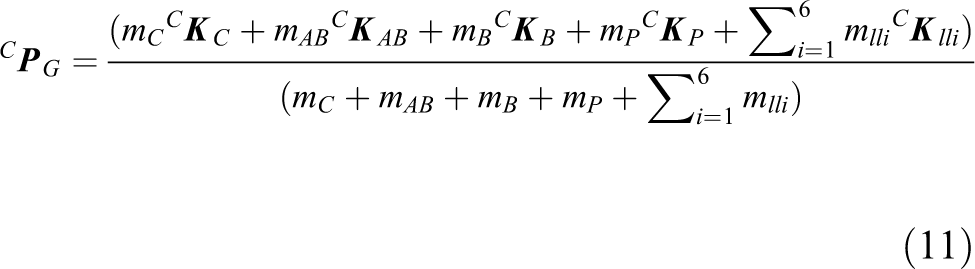
\begin{array}{l} {}^{C}P_{G} = \frac{(m_{C} {}^{C}K_{C} + m_{A B} {}^{C}K_{A B} + m_{B} {}^{C}K_{B} + m_{P} {}^{C}K_{P} + \sum_{i = 1}^{6} m_{l l i} {}^{C}K_{l l i})}{(m_{C} + m_{A B} + m_{B} + m_{P} + \sum_{i = 1}^{6} m_{l l i})} \end{array}

where m_* represents the mass of the mechanism and is denoted by the right subscript. * K _* represents the barycenter of the mechanism and is denoted by the right subscript, with respect to the reference coordinate system (left superscript). The symbols C, AB, B, P, and lli in the subscript, respectively, denote the start frame, A-B rotator, base platform of the Stewart manipulator, active platform of the Stewart manipulator, and the ith leg of the Stewart manipulator. The barycenters of the specific mechanism are expressed as

{\begin{cases} {}^{C}K_{A B} = {}^{C}R_{A B} {}^{A B}K_{A B} + {}^{C}P_{A B} \\ {}^{C}K_{B} = {}^{C}R_{A B} ({}^{A B}R_{B} {}^{B}K_{B} + {}^{A B}P_{B}) + {}^{C}P_{A B} \\ {}^{C}K_{P} = {}^{C}R_{A B} ({}^{A B}R_{B} ({}^{B}R_{P} {}^{P}K_{P}) + {}^{A B}P_{B}) + {}^{C}P_{A B} \\ {}^{C}K_{l l i} = {}^{C}R_{A B} ({}^{A B}R_{B} {}^{B}K_{l l i} + {}^{A B}P_{B}) + {}^{C}P_{A B} \end{cases}

where ^B K _lli is obtained by Stewart inverse kinematics. ^AB R _B is an identity matrix. ^C R _AB and ^B R _P are obtained in the following section. Other variables are constants determined by the mechanism parameters.

FSS pose distribution algorithm

Back-illuminated strategy

During the observation, the active reflector is controlled as a parabolic surface, and the flare angle of the receiver is constant. The receiver is controlled to move on the focal surface. The receiver shape is similar to a horn, and its receptive field is limited by the structure. When the receiver moves to some point where the theoretical tilt angle is larger than a given threshold, part of its receptive field will be outside the active reflector surface, which weakens the intensity of the signal detected by the receiver, as shown in Figure 6. To alleviate this situation, the back-illuminated strategy is proposed.

Figure 6.

Schematic diagram of the back-illuminated strategy of the receiver.

Normally, the center normal vector of the receiver must pass through the spherical center of the active reflector, as shown in the normal-illuminated triangle in Figure 6. However, when the receiver must be back-illuminated, the center normal vector of the receiver is only required to intersect with the Z_G-axis, as shown in the back-illuminated triangle in Figure 6.

When the theoretical tilt angle of receiver θ ₀ is larger than threshold θ_th , the actual tilt angle of receiver θ can be expressed as

θ = θ_{0} - θ_{H}

where θ_H is the back-illuminated angle, which can be expressed as

θ_{H} = θ_{d} - θ_{p} - θ_{q}

where

{\begin{cases} θ_{d} = arcsin (R_{r} / (2 \cdot d_{l})) \\ d_{l} = \sqrt{R^{2} + {(R (1 - f))}^{2} - 2 R^{2} (1 - f) \cdot cos θ_{r}} \\ θ_{r} = arcsin (R_{r} / (2 \cdot R)) \\ θ_{p} = arcsin (R_{d} / (2 \cdot R)) - θ_{0} \\ θ_{q} = arcsin (R \cdot (1 - f) \cdot sin (θ_{p}) / d) \\ d = \sqrt{R^{2} + {(R (1 - f))}^{2} - 2 R^{2} (1 - f) \cdot cos θ_{p}} \end{cases}

The threshold value of the tilt angle θ _th can be expressed as

θ_{th} = arcsin (R_{d} / (2 R)) - θ_{r}

where R, R_d , R_r , and f, respectively, represent the active reflector radius, the effective aperture of the active reflector, the illumination caliber of the receiver, and the ratio between the height of the focal surface and R.

Pose distribution for the FSS

As shown in Figure 2, the pose of the receiver is determined by the pose of the star frame, angles of the A-B rotator, and status of the rigid Stewart manipulator. The Stewart keeps in initial state during the FSS pose distribution, thus, given the position of the receiver, and the attitude of the star frame is determined when given angles of the A-B rotator. It is obvious that there is attitude distribution redundancy between the CDPR and the A-B rotator. In addition, the A-B rotator cannot fully compensate for the rotation of 3-DOF for its special structure. Thus, the receiver pose should be properly allocated to the CDPR and A-B rotator.

Previous studies examined the pose distribution algorithm, and the rigid Stewart manipulator was used to compensate for the theoretical attitude angle of the receiver, for which the A-B rotator could not compensate.¹⁶ However, this approach limits the compensation space of the rigid Stewart manipulator and makes it difficult to compensate the position and attitude deviation of the receiver caused by external disturbances. Meanwhile, the FSS is prone to vibration under the action of the rigid Stewart manipulator⁸; thus, the fewer poses of the rigid Stewart manipulator to be adjusted, the better.

In this section, a pose distribution algorithm that ensures the accuracy of the receiver pose is proposed, and its flowchart is shown in Figure 7.

Figure 7.

Flowchart of the pose distribution algorithm.

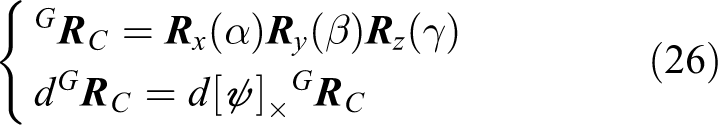
The attitude matrix calculated by using the vector and rotation angle is defined as

R (n, ϑ) = I + sin ϑ {[n]}_{\times} + (1 - cos ϑ) {[n]}_{\times}^{2}

where [ n ]_× is the skew-symmetric matrix of vector n .

Given the position of receiver ^G P _R , the theoretical target tilt angle of receiver θ ₀ can be expressed as

θ_{0} = arccos (- [\begin{matrix} 0 & 0 & 1 \end{matrix}] {}^{G}P_{R} / | | {}^{G}P_{R} | |)

Considering the back-illuminated strategy of the receiver, the actual tilt angle of receiver θ is given by

θ = {\begin{cases} θ_{0}, θ_{0} \leq θ_{th} \\ θ_{0} - θ_{H}, θ_{0} > θ_{th} \end{cases}

where θ_H and θ _th can be obtained through equations (13) and (14), respectively. The attitude of the active platform of Stewart ^G R _P , which equals to ^G R _R , can be obtained by

{}^{G}R_{P} = R (({}^{G}P_{R} \times {[\begin{matrix} 0 & 0 & 1 \end{matrix}]}^{T}), θ)

^G R _P is calculated first; thus, the receiver pose can be ensured in this pose distribution algorithm.

Given the rotation angles of the A-B rotator, θ_A and θ_B , the attitude of the A-B rotator to compensate is shown as

{}^{C}R_{A B} = R_{X} (θ_{A}) R_{Y} (θ_{B})

where R _x (θ) and R _y (θ) are the rotation matrixes that, respectively, rotate around the x and y axes.

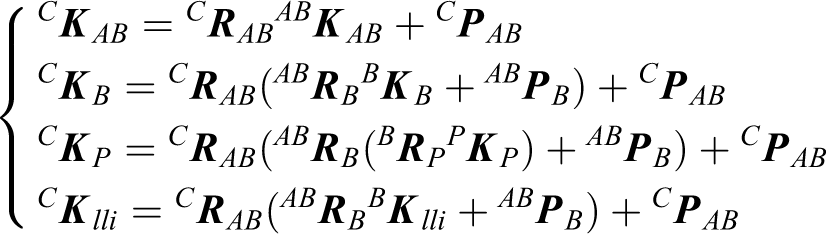
The positions ^G P _P , ^G P _AB , and ^G P _C can be expressed as

{\begin{cases} {}^{G}P_{P} = {}^{G}P_{R} - {}^{G}R_{P} {}^{P}P_{R} \\ {}^{G}P_{A B} = {}^{G}P_{P} - {}^{G}R_{B} {}^{B}P_{P} + {}^{G}R_{B} {}^{B}P_{A B} \\ {}^{G}P_{C} = {}^{G}P_{A B} - {}^{G}R_{C} {}^{C}P_{A B} \\ {}^{G}R_{B} = {}^{G}R_{P} {}^{B}R {^{- 1}}_{P} \\ {}^{G}R_{C} = {}^{G}R_{P} {({}^{C}R_{A B} {}^{A B}R_{B} {}^{B}R_{P})}^{- 1} \end{cases}

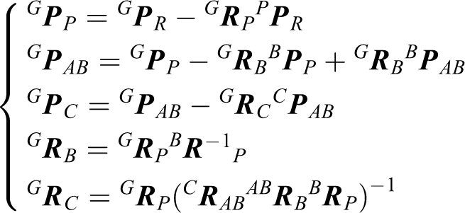
Because the rigid Stewart manipulator is maintained in the initial state during the pose distribution, ^B R _P and ^AB R _B are identity matrices. Moreover, ^B P _P , ^B P _AB , ^P P _R , and ^C P _AB are constant vectors determined by the mechanism parameters of the feed cabin.

The values of ^C P _G , ^G R _C , and ^G P _C are determined by the position of receiver ^G P _R and the rotation angles of the A-B rotator, θ_A and θ_B . Substituting these variables and the time-varying barycenter of the feed cabin ^C P _G back into equation (1), the cable tension ^G T _Bi and cable length L_i are obtained.

The receiver pose is distributed to the star frame and the A-B rotator. Given the position of the receiver ^G P _R , it is obvious that the difference value of θ_A and θ_B will obtain the difference pose of the star frame, and the resultant cable tensions will be different. Therefore, to ensure the position and attitude accuracy of the receiver and the stability of the FSS, the pose optimal distribution problem can be changed to an optimization problem of the A-B rotator rotation angles. The following sections focus on solving this problem.

Multi-objective optimization for pose distribution

In previous studies, the minimum variance of cable tensions¹⁶ and the stiffness²³ of the CDPR were, respectively, used to evaluate the stability of a system. The variance of cable tensions indicates the distribution of the six cable forces, and its minimum makes the values of cable tensions identical. The greater is the variance of cable tensions, the more dispersed is the cable tension distribution. Furthermore, the more difficult it is for the CDPR to coordinate control, the more likely it is that the rope will virtually pull, which results in a loss in stability.²⁴ The stiffness represents the ability of the system to resist the external forces, for example, the disturbances from the wind. So under the external disturbances, the greater is the system stiffness, the higher is the trajectory accuracy of the end effector (the receiver), and the more stable is the system.²³ Consequently, a system higher stiffness means a higher stability.

In this section, the objective functions of tension and stiffness are derived, and multiple performances of variance of cable tensions and stiffness of the CDPR are simultaneously considered for optimization of the rotation angles of the A-B rotator.

FSS tension objective function

Owing to its flexibility, the FSS is prone to swaying when the cable tensions are unevenly distributed. Moreover, some cables tend to be in a virtual traction state with a large variance of the cable tensions. Thus, the smaller variance of cable tensions makes the FSS more stable. In this part, the minimum variance of six cable tensions is selected to be the tension objective function, which is described as

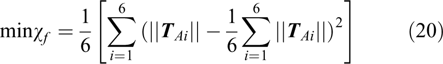
min χ_{f} = \frac{1}{6} [\sum_{i = 1}^{6} {(‖ T_{A i} ‖ - \frac{1}{6} \sum_{i = 1}^{6} ‖ T_{A i} ‖)}^{2}]

where || T _Ai || is the modulus of vector T _Ai .

Stiffness objective functions for the FSS

To assess the elastic response of a robot to an external wrench, it is important to define the stiffness indices. The stiffness matrix refers to the relationship between the wrench and the deflection.²⁵ When the system is in a static equilibrium state, deflection of the end effector is determined by providing a wrench to the end effector of a robot.

As shown in Figure 5, we add a virtual y-axis in {T_i }. Accordingly, the rotation matrix from {T_i } to {G} can be expressed as

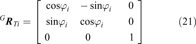
{}^{G}R_{T i} = [\begin{array}{l} \begin{matrix} cos φ_{i} & - sin φ_{i} & 0 \end{matrix} \\ \begin{matrix} sin φ_{i} & cos φ_{i} & 0 \end{matrix} \\ \begin{matrix} 0 & 0 & 1 \end{matrix} \end{array}]

The cable tension with respect to {G} can be expressed as

{}^{G}T_{B i} = {}^{G}R_{T i} {}^{T i}T_{B i}

{}^{T i}T_{B i} = {[\begin{matrix} F_{H i} & 0 & F_{i B_V} \end{matrix}]}^{T}

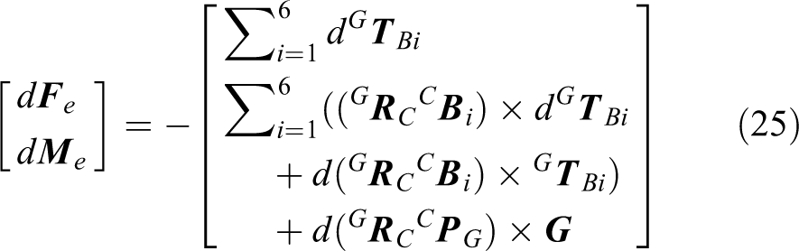
According to equation (1), to ensure the FSS equilibrium, the external force and moments acting on the feed cabin can be described as

[\begin{array}{l} F_{e} \\ M_{e} \end{array}] = - [\begin{array}{l} \sum_{i = 1}^{6} {}^{G}T_{B i} + G \\ \sum_{i = 1}^{6} ({}^{G}R_{C} {}^{C}B_{i}) \times {}^{G}T_{B i} + M_{G} \end{array}]

The differential of equation (24) can be expressed as

[\begin{array}{l} d F_{e} \\ d M_{e} \end{array}] = - [\begin{array}{l} \sum_{i = 1}^{6} d {}^{G}T_{B i} \\ \sum_{i = 1}^{6} (({}^{G}R_{C} {}^{C}B_{i}) \times d {}^{G}T_{B i} \\ + d ({}^{G}R_{C} {}^{C}B_{i}) \times {}^{G}T_{B i}) \\ + d ({}^{G}R_{C} {}^{C}P_{G}) \times G \end{array}]

Let the position and attitude of the star frame be expressed in a spiral vector S = [ r ^T , ψ ^T ] ^T , where r ^T = ^G P _C ^T = [ x, y, z ], and ψ ^T = [ α, β, γ ] is the Euler angles vector for the star frame. The rotation matrix ^G R _C and its differential can be described as²⁶

{\begin{cases} {}^{G}R_{C} = R_{x} (α) R_{y} (β) R_{z} (γ) \\ d {}^{G}R_{C} = d {[ψ]}_{\times} {}^{G}R_{C} \end{cases}

When the feed cabin suffers an infinitesimal deflection dS = [ dr ^T , dψ ^T ] ^T , the differential of ^G B _i (equal to ^G P _C + ^G R _C ^C B _i ) can be described as

\begin{array}{l} d {}^{G}B_{i} = d {[ψ]}_{\times} {}^{G}R_{C} {}^{C}B_{i} + d {}^{G}P_{C} \\ = [{\begin{matrix} I & - [{}^{G}R_{C} {}^{C}B_{i}] \end{matrix}}_{\times}] d S \end{array}

Let R _cont = [0, −1, 0;1, 0, 0;0, 0, 0], ^Ti L _i = [ l_i , 0, h_i ] ^T , V _x = [1, 0, 0], and V _y = [0, 1, 0]. Note that ^G L _Ti = ^G R _Ti ^Ti L _i and ^G L _Ti =^G A _i− ^G B _i . Taking the differential of tanφ_i = ( V _y ^G T _Ti )/( V _x ^G T _Ti ), cosφ_i = ( V _x ^G T _Ti )/√(( V _x ^G T _Ti )( V _x ^G T _Ti ) + ( V _y ^G T _Ti )( V _y ^G T _Ti )), and equation (21), we can obtain

\begin{array}{l} d φ_{i} = \\ {\begin{matrix} \begin{array}{l} {cos}^{2} φ_{i} (V_{y} {}^{G}T_{T i} V_{x} - V_{x} {}^{G}T_{T i} V_{y}) d {}^{G}B_{i} \\ / {(V_{x} {}^{G}T_{T i})}^{2}, φ_{i} \neq 90^{\circ}, 270^{\circ} \end{array} \\ \begin{array}{l} (1 / sin φ_{i}) (V_{x} / l_{i} - V_{x} {}^{G}T_{T i} (V_{x} {}^{G}T_{T i} V_{x} \\ + V_{y} {}^{G}T_{T i} V_{y}) / l_{i}^{3}) d {}^{G}B_{i}, φ_{i} = 90^{\circ}, 270^{\circ} \end{array} \end{matrix} \end{array}

d {}^{G}R_{T i} = R_{cont} {}^{G}R_{T i} d φ_{i} = R_{cont} {}^{G}R_{T i} R_{d R} d S

where R _dR can be easily derived from equations (28) and (29).

The value of l_i and h_i can be expressed as follows by considering the cables as inextensible catenaries²⁷

{\begin{cases} l_{i} = \frac{F_{H i}}{q} ln (\frac{F_{i A_V} + ‖ T_{A i} ‖}{F_{i B_V} + ‖ T_{B i} ‖}) \\ h_{i} = \frac{1}{q} (‖ T_{A i} ‖ - ‖ T_{B i} ‖) \end{cases}

Taking the differentiation of equation (30), the stiffness matrix of the ith cable can be expressed as

{\begin{cases} [\begin{array}{l} d F_{H i} \\ d F_{i B_V} \end{array}] = k_{i}^{c} [\begin{matrix} d l_{i} \\ d h_{i} \end{matrix}] = {[\begin{array}{l} \begin{matrix} \frac{\partial l_{i}}{\partial F_{H i}} & \frac{\partial l_{i}}{\partial F_{i B_V}} \end{matrix} \\ \begin{matrix} \frac{\partial h_{i}}{\partial F_{H i}} & \frac{\partial h_{i}}{\partial F_{i B_V}} \end{matrix} \end{array}]}^{- 1} [\begin{matrix} d l_{i} \\ d h_{i} \end{matrix}] \\ \frac{\partial l_{i}}{\partial F_{H i}} = \frac{l_{i}}{F_{H i}} - \frac{1}{q} (\frac{F_{i A_V}}{‖ T_{A i} ‖} - \frac{F_{i B_V}}{‖ T_{B i} ‖}) \\ \frac{\partial l_{i}}{\partial F_{i B_V}} = \frac{\partial h_{i}}{\partial F_{H i}} = \frac{F_{H i}}{q} (\frac{1}{‖ T_{A i} ‖} - \frac{1}{‖ T_{B i} ‖}) \\ \frac{\partial h_{i}}{\partial F_{i B_V}} = \frac{1}{q} (\frac{F_{i A_V}}{‖ T_{A i} ‖} - \frac{F_{i B_V}}{‖ T_{B i} ‖}) \end{cases}

Let k ^c _i = [ k^c _i ₁, k^c _i ₂; k^c _i ₃, k^c _i ₄ ] and K ^c _i = [ k^c _i ₁,0, k^c _i ₂; 0,0,0;k^c _i ₃,0, k^c _i ₄]. Moreover, note that ^G R _Ti ^Ti L _i = ^G A _i−^G B _i . Hence, the stiffness matrix of a single cable can be described as

\begin{array}{l} d {}^{T i}T_{B i} \\ = K_{i}^{c} d {}^{T i}L_{i} \\ = K_{i}^{c} {}^{G}R_{T i} (- d {}^{G}B_{i} - d {}^{G}R_{T i} {}^{T i}L_{i}) \\ = K_{i}^{c} {}^{G}R_{T i} (- [{\begin{matrix} I & - [{}^{G}R_{C} {}^{C}B_{i}] \end{matrix}}_{\times}] - \\ R_{cont} {}^{G}R_{T i} {}^{T i}L_{i} R_{d R}) d S \end{array}

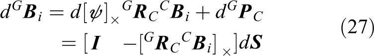
Taking the differentiation of equation (22), and substituting equations (29) and (32) into it, we can get

\begin{array}{l} d {}^{G}T_{B i} \\ = d {}^{G}R_{T i} {}^{T i}T_{B i} + {}^{G}R_{T i} d {}^{T i}T_{B i} \\ = R_{cont} {}^{G}R_{T i} {}^{T i}T_{B i} R_{d R} d S - {}^{G}R_{T i} K_{i}^{c} {}^{G}R_{T i} \\ ([{\begin{matrix} I & - [{}^{G}R_{C} {}^{C}B_{i}] \end{matrix}}_{\times}] + R_{cont} {}^{G}R_{T i} {}^{T i}L_{i} R_{d R}) d S \\ = K_{e q_i}^{F} d S \end{array}

Substituting equation (33) into equation (25), we can get

d F_{e} = - \sum_{i = 0}^{6} K_{e q_i}^{F} d S = K_{e q}^{F} d S

Note that

\begin{array}{l} d ({}^{G}R_{C} {}^{C}B_{i}) \times {}^{G}T_{B i} \\ = d {[ψ]}_{\times} ({}^{G}R_{C} {}^{C}B_{i}) \times {}^{G}T_{B i} \\ = - ({[{}^{G}R_{C} {}^{C}B_{i}]}_{\times} d ψ) \times {}^{G}T_{B i} \\ = - {[[\begin{matrix} 0_{3 \times 3} & {[{}^{G}R_{C} {}^{C}B_{i}]}_{\times} \end{matrix}] d S]}_{\times} {}^{G}T_{B i} \\ = - K_{T i} d S \end{array}

Additionally,

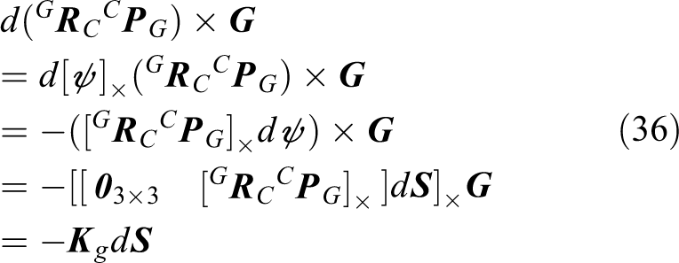
\begin{array}{l} d ({}^{G}R_{C} {}^{C}P_{G}) \times G \\ = d {[ψ]}_{\times} ({}^{G}R_{C} {}^{C}P_{G}) \times G \\ = - ({[{}^{G}R_{C} {}^{C}P_{G}]}_{\times} d ψ) \times G \\ = - {[[\begin{matrix} 0_{3 \times 3} & {[{}^{G}R_{C} {}^{C}P_{G}]}_{\times} \end{matrix}] d S]}_{\times} G \\ = - K_{g} d S \end{array}

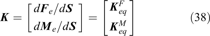
where K _Ti and K _g can be easily derived from equations (35) and (36).

Substituting equations (35) and (36) into equation (25), we can obtain

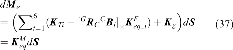
\begin{array}{l} d M_{e} \\ = (\sum_{i = 1}^{6} (K_{T i} - {[{}^{G}R_{C} {}^{C}B_{i}]}_{\times} K_{e q_i}^{F}) + K_{g}) d S \\ = K_{e q}^{M} d S \end{array}

Thus, the FSS stiffness can be expressed as

K = [\begin{array}{l} d F_{e} / d S \\ d M_{e} / d S \end{array}] = [\begin{array}{l} K_{e q}^{F} \\ K_{e q}^{M} \end{array}]

However, the stiffness matrix is a 6 × 6 matrix whose components have different units. To define the stiffness performance indices, we should first nondimensionalize the stiffness matrix.

Let

K = [\begin{array}{l} \begin{matrix} K_{11} & K_{12} \end{matrix} \\ \begin{matrix} K_{21} & K_{22} \end{matrix} \end{array}]

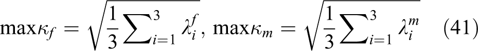
The means of the eigenvalue of G _f G ^T _f and G _m G ^T _m , denoted by {λ^f _i }³ ₁ and {λ^m _i }³ ₁, are used to define the translational κ_f and rotation κ_m stiffness performance indices, respectively²⁸

κ_{f} = \sqrt{\frac{1}{3} \sum_{i = 1}^{3} λ_{i}^{f}}, κ_{m} = \sqrt{\frac{1}{3} \sum_{i = 1}^{3} λ_{i}^{m}}

where G _f = [ K ₁₁ S _r , K ₁₂ S _ψ ] and G _m = [ K ₂₁ H _r , K ₂₂ H _ψ ].

Here, S _r, S _ψ, H _r , and H _ψ are orthogonal matrices whose columns are the eigenvectors of matrices K ^T ₁₁ K ₁₁, K ^T ₁₂ K ₁₂, K ^T ₂₁ K ₂₁, and K ^T ₂₂ K ₂₂, respectively.

According to the definition of stiffness, the larger κ_f and κ_m make the FSS more stable. Therefore, the maximum values of κ_f and κ_m are selected to be the stiffness objective functions, which can be described as

max κ_{f} = \sqrt{\frac{1}{3} \sum_{i = 1}^{3} λ_{i}^{f}}, max κ_{m} = \sqrt{\frac{1}{3} \sum_{i = 1}^{3} λ_{i}^{m}}

GA-based multi-objective optimization

The genetic algorithm (GA) is a global method for solving optimization problems based on natural evolution.^29,30 To solve the optimization of the rotation angles of the A-B rotator, GA is adopted because of its good performance in searching in complex objective functions.³¹

The functions χ_f , κ_f, and κ_m are very important indices for evaluating FSS stability. The tension objective function {min χ_f } makes the cable tensions evenly allocated; however, it cannot ensure that the FSS has sufficient stiffness. Conversely, the objective functions {max κ_f } and {max κ_m } enable the FSS to have sufficient stiffness; however, it cannot ensure that the cable tensions are evenly distributed. To make the FSS more stable, a multi-objective pose optimal distribution algorithm for the FSS is designed. Its mathematical description is given as follows

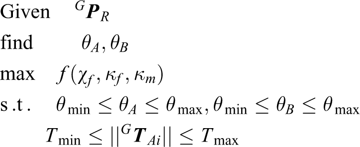
\begin{array}{l} Given {}^{G}P_{R} \\ find θ_{A}, θ_{B} \\ max f (χ_{f}, κ_{f}, κ_{m}) \\ s.t. θ_{min} \leq θ_{A} \leq θ_{max}, θ_{min} \leq θ_{B} \leq θ_{max} \\ T_{min} \leq ‖ {}^{G}T_{A i} ‖ \leq T_{max} \end{array}

where T _min = 1000 N and T _max = 400,000 N are the minimum and maximum cable tensions, respectively, and θ _min = −18° and θ _max = 18° are the minimum and maximum angles of the A-B rotator, respectively. Because the values of χ_f , κ_f , and κ_m have different ranges, we normalize them first. The multi-objective function is expressed as

f (χ_{f}, κ_{f}, κ_{m}) = ω_{1} (1 - {}^{-}χ_{f}) + ω_{2} {}^{-}κ_{f} + ω_{3} {}^{-}κ_{m}

{\begin{cases} {}^{-}χ_{f} = (χ_{f} - χ_{f min}) / (χ_{f max} - χ_{f min}) \\ {}^{-}κ_{f} = (κ_{f} - κ_{f min}) / (κ_{f max} - κ_{f min}) \\ {}^{-}κ_{m} = (κ_{m} - κ_{m min}) / (κ_{m max} - κ_{m min}) \end{cases}

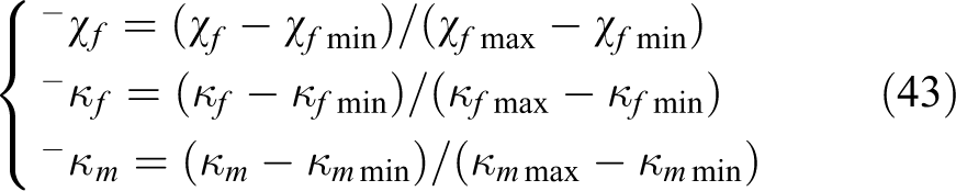
where ^- χ_f , ^- κ_f , and ^- κ_m are the normalized expression of χ_f , κ_f , and κ_m , respectively. χ_f _min, κ_f _min, and κ_m _min are the minimum values of χ_f , κ_f , and κ_m in the feasible domain, respectively. χ_f _max, κ_f _max, and κ_m _max are the maximum values of χ_f , κ_f , and κ_m in the feasible domain, respectively. These minimum and maximum values are calculated before the GA iteration using grid searching method. ω ₁, ω ₂, and ω ₃ are weight factors and ω ₁ + ω ₂ + ω ₃ = 1.

The values of ω₁ , ω ₂, and ω ₃ are positive numbers less than one. The solution of a multi-objective optimal problem is not unique but there exists a Pareto-optimal solution; the choice of one solution over the other requires problem knowledge.³² The selection of the weight factors mainly depends on whether the FSS is preferred to be stiff or the variance of the cable tensions. Because ^- κ_f and ^- κ_m are all the stiffness indices, they account for the same proportion of optimization task. ^- χ_f indicates whether the FSS is loss in stability. From the view of the system safety, ^- χ_f should be cared much more than ^- κ_f and ^- κ_m . On the premise of ω ₁ > ω ₂ and ω ₂ = ω₃, the sequence search method is used to determine the weight factors. The final weight factors of ω ₁ = 0.6 and ω ₂ = ω ₃ = 0.2 can obtain smooth angles of the A-B rotator and retains a low variance of cable tensions and high FSS stiffness.

Numerical simulation and discussion

The main parameters of the FSS are listed in Table 1. In the GA, the population size is set to 60, and the maximum number of generations is set to 100.

Table 1.

Main FSS parameters.

Parameter	Physical meaning	Value
q	Weight per unit cable length	15 kg/m
R_T	Radius of the tower circle	300 m
R_C	Radius of the circle formed by anchor nodes B_i	6.5 m
R	Radius of curvature of the main reflector	300 m
R_d	Effective caliber of the active reflector	500 m
R_r	Illumination caliber of the receiver	300 m
f	Ratio between height of the focal surface and R	0.4611
β_c	Central angle between two closets B_i	5.289°
^C P _AB	Translation vector of coordinate system {AB} with respect to {C}	[0;0;−0.5] m
^B P _AB	Translation vector of coordinate system {AB} with respect to {B}	[0;0;−0.62] m
^P P _B	Translation vector of coordinate system {AB} with respect to {P}	[0;0;1.75] m
^AB P _P	Translation vector of coordinate system {P} with respect to {AB}	[0;0;−1.13] m
^P P _R	Coordinate of the receiver with respect to {P}	[0;0;−1.10] m
m_G	Mass of the feed cabin	29583 kg
m_C	Mass of the star frame	19473 kg
m_AB	Mass of the A-B rotator	3405 kg
m_B	Mass of the base platform of Stewart	2805 kg
m_P	Mass of the active platform of Stewart	2475 kg
m_L	Mass of each leg of Stewart	230 kg

FSS: feed support system.

To fully demonstrate the performance of the pose distribution method of the FSS, a typical test path is chosen for the experiment, as shown in Figure 8. The test path is an arc attached to the focal surface, and it passes through the lowest point of the focal surface from southwest to northeast. In the following simulation figures, when the abscissa is negative, the test path is in the seventh octant of the global coordinate system, and the theoretical tilt angles of the receiver θ ₀ are the opposite of the abscissa values.

Figure 8.

Test path for the pose distribution method of the FSS. FSS: feed support system.

In the experiment, the proposed multi-objective pose optimal distribution algorithm is compared with another method. Algorithm 1 directly uses the 3:5 tilt angle distributions between the CDPR and A-B rotator, which is proposed by Deng et al.³³ In this algorithm, the angles of the A-B rotator θ_A and θ_B are equal to the corresponding element in the matrix product R _x (θ_A ) R _y (θ_B ) R _z (θ_Z ), which is used to decompose the attitude matrix ^C R^’ _AB = R(( ^G P _R × [0,0,1] ^T ),(θ−3θ ₀ /8)). Algorithm 2 uses the GA-based multi-objective pose optimal distribution method proposed in this article.

The GA iterative convergence process is shown in Figure 9. It is observed that the GA converges after 40 generations. The angles of the A-B rotator and the cable tensions are shown in Figure 10. The A-B rotator angles continuously vary in the two algorithms. When the theoretical tilt angle of the receiver is greater than θ _th = 26.45°, the receiver begins to back illuminate, and the angles of the A-B rotator begins to decrease. From the view of Figure 10(a) and (c), the maximum angles of the A-B rotator are less than 18°, which is the limit position that the A-B rotator can reach. The angles of the A-B rotator will transcend the limit without using the back-illuminated strategy. As shown in Figure 10(b) and (d), the distribution of cable tensions in algorithm 2 is more compact than algorithm 1, and the minimum cable tensions of algorithm 2 are greater than that of algorithm 1. The more dispersed is the cable tension distribution, the more difficult it is for the CDPR to coordinate control, and the more likely it is that the rope will virtually pull. Consequently, the algorithm 2 can provide the FSS with greater stability.

Figure 9.

Iterative convergence process of GA. GA: genetic algorithm.

Figure 10.

Angles of the A-B rotator and cable tensions of the test path. (a) Angles of the A-B rotator with algorithm 1, (b) cable tensions with algorithm 1, (c) angles of the A-B rotator with algorithm 2, and (d) cable tensions with algorithm 2.

The curves shown in Figure 11 demonstrate that algorithm 2 performs better than algorithm 1 in χ_f , κ_f , and κ_m . The red and green curves represent the percentage increases in the translational stiffness and the rotation stiffness, respectively, while the blue one represents the percentage increases in the variance of cable tensions. It is obvious that algorithm 2 can provide a greater translational stiffness and rotation stiffness than algorithm 1 in most poses. There is minimal difference in stiffness when the receiver moves near the center of the focal surface, whereas a significant difference exists when the receiver begins to back illuminate. The maximum percentage increase in the translational stiffness is up to 46% and 22% for rotation stiffness. In some points, to provide greater stability, the objective values of the stiffness that algorithm 2 is lower than algorithm 1 are compensated by the smaller variance of cable tensions. From the view of the stiffness and the variance of cable tensions, the FSS can provide a greater stability with algorithm 2.

Figure 11.

Percentage increase curves of κ_f , κ_m , and χ_f by algorithm 2.

Conclusions and future work

In this article, the back-illuminated strategy of the receiver and the dimensionless stiffness of the FSS were derived in detail. A pose distribution method that ensures the accuracy of the position and attitude of the receiver was designed. Using the weighted sum of the variance of cable tensions and the dimensionless stiffness of the FSS as objective functions, a multi-objective pose optimal distribution algorithm for the FSS was proposed. Compared with the pose distribution algorithm by Deng et al.,³³ the proposed algorithm not only ensures the position and attitude accuracy of the receiver but also retains a lower variance of cable tensions and higher stiffness of the FSS, which are crucial to the stability of the FSS.

To find out the optimal set, we employ an empirical method to determine the weight factors in equation (42) and carry out a lot of trials and finally achieve a good performance. We are planning to explore deeper correlation between these weight factors and adopt adaptive methods in our future work.

Footnotes

Acknowledgement

The authors would like to thank Professor Junzhi Yu from the Institute of Automation, Chinese Academy of Sciences, for providing great suggestions and to the anonymous reviewers for their valuable comments on the previous versions of the article.

Declaration of conflicting interests

The authors declared no potential conflicts of interest with respect to the research, authorship, and/or publication of this article.

Funding

The authors disclosed receipt of the following financial support for the research, authorship, and/or publication of this article: This work was supported by the National Nature Science Foundation of China (no 61573358).

ORCID iD

Sai Deng

References

Nan

. Five hundred meter aperture spherical radio telescope (FAST). Sci China Ser G 2006; 49(2): 129–148.

. China hopes to move FAST on largest telescope. Science 1998; 281(5378): 771–773.

Shao

Tang

Chen

. Driving force analysis for the secondary adjustable system in FAST. Robotica 2011; 29(6): 903–915.

Deng

Jing

Yang

. Research on trajectory planning of on-the-fly observing for the active feed receiver in FAST. In: IEEE Chinese control conference, Hangzhou, China, 28 July–30 July 2015, pp. 4393–4399. IEEE.

Chai

Tang

. Error modeling and accuracy analysis of a multi-level hybrid support robot. Robotics and automation. In: IEEE international conference on robotics and automation, Saint Paul, USA, 14 May–18 May 2012, pp. 2319–2324. IEEE.

Shao

Tang

Wang

. A fuzzy PID approach for the vibration control of the FSPM. Int J Adv Robot Syst 2013; 10: 1.

Zhu

Pan

. Mechanics in the feed support of FAST telescope and its research progress. Adv Mech 2011; 41(2): 133–154.

Tang

Liu

Shao

. Self-excited vibration analysis for the feed support system in FAST. Int J Adv Robot Syst 2014; 11(1): 1.

Duan

Qiu

. Nonlinear static analysis and cable-length solution of a cabin-cable system. Mech Sci Technol 2006; 25(8): 946–971.

10.

Qiu

Peng

. Nonlinear mechanics analysis of the suspended feed structure of the largest radio telescope. J Xidian Univ Natural Sci Ed 2000; 27(4): 452–455.

11.

Kozak

Zhou

Wang

. Static analysis of cable-driven manipulators with non-negligible cable mass. IEEE Trans Rob 2006; 22(3): 425–433.

12.

Tang

Shao

. Trajectory generation and tracking control of a multi-level hybrid support manipulator in FAST. Mechatronics 2013; 23(8): 1113–1122.

13.

Huang

Zhu

Tang

. Analysis and a simplified model of the cable of a large-scale flexible parallel manipulator for a large radio telescope. Astron Res Technol 2013; 10(1): 77–84.

14.

Zhu

Pan

. Equilibrium analysis of FAST rope-drive parallel manipulator based on rope force optimization. Eng Mech 2011; 28(4): 185–157.

15.

Chai

Tang

Shao

. Terminal accuracy analysis of a multi-level hybrid support system based on time-varying barycenter. Robot 2011; 33(5): 546–552.

16.

Nan

Kärcher

. Working space analysis and optimization of the main positioning system of FAST cabin suspension. In: Conference on ground-based and airborne instrumentation for astronomy II, Marseille, France, 23–28 June 2008, pp. 70120T.1–70120T.11.

17.

Yao

Zhu

Sun

. Pose planning for the feed support system of FAST. Adv Mech Eng 2014; 2014(1): 1–9.

18.

Shao

Tang

Wang

. Dynamic modeling and wind vibration control of the feed support system in FAST. Nonli Dyn 2011; 67(2): 965–985.

19.

. Static stiffness analysis of flexible-cable-driven parallel mechanism. J Mech Eng 2010; 46(3): 8–16.

20.

Raid

. Some modeling aspects in the nonlinear finite element analysis of cable supported bridges. Comput Struct 1999; 71(4): 397–412.

21.

. Mechanics analysis and control research of the feed tracking system for super antenna. PhD Thesis, Xidian University, China, 2007.

22.

Yao

Tang

Wang

. Dimensional optimization design of the four-cable-driven parallel manipulator in Fast. IEEE/ASME Trans Mech 2010; 15(6): 932–941.

23.

Wei

Qiu

Yang

. An approach to evaluate stability for cable-based parallel camera robots with hybrid tension-stiffness properties. Int J Adv Robot Syst 2015, 12: 1.

24.

Sun

. Study on non-linear static, kinematics and dynamics of cable and cabin system for large radio telescope. PhD Thesis, Xidian University, China, 2001.

25.

Moradi

. Stiffness analysis of cable-driven parallel robots. PhD Thesis, Queen’s University, Canada, 2013.

26.

Hamano

Derivative of rotation matrix direct matrix derivation of well-known formula. In: Proceeding of green energy and systems conference, Long Beach, USA, 25 November 2013. SPIE.

27.

Jayaraman

Knudson

. A curved element for the analysis of cable structures. Comput Struct 1981; 14(3): 325–333.

28.

Taghvaeipour

Angeles

Lessard

. Online computation of the stiffness matrix in robotic structures using finite element analysis. Report, McGill University, Canada, 2010.

29.

. GA-based multi-objective optimal design of a planar 3-DOF cable-driven parallel manipulator. In: IEEE international conference on robotics and biomimetics, >Kunming, China, 17–20 December 2006, pp. 1360–1365. IEEE.

30.

Liu

Liang

. Non-holonomic path planning of a free-floating space robotic system using genetic algorithms. Adv Rob 2008; 22(4): 451–476.

31.

Houck

Joines

JA,

Kay

. A genetic algorithm for function optimization: a MATLAB implementation. NCSUIE TR 1995; 95.09.

32.

Srinivas

Deb

. Muiltiobjective optimization using nondominated sorting in genetic algorithms. Evolut Comput 2014; 2(3): 221–248.

33.

Deng

Jing

Yang

. Research on pose distribution algorithms of the feed support system in FAST. Opt Prec Eng 2017; 25(2): 375–384.

Multi-objective pose optimal distribution method for the feed support system of Five-hundred-meter Aperture Spherical radio Telescope

Abstract

Keywords

Introduction

FSS description and modeling

Description of the FSS

CDPR static equilibrium equation

Suspension cable modeling

Time-varying barycenter

FSS pose distribution algorithm

Back-illuminated strategy

Pose distribution for the FSS

Multi-objective optimization for pose distribution

FSS tension objective function

Stiffness objective functions for the FSS

GA-based multi-objective optimization

Numerical simulation and discussion

Conclusions and future work

Footnotes

Acknowledgement

Declaration of conflicting interests

Funding

ORCID iD

References