Sage Journals: Discover world-class research

Abstract

Object recognition is one of the essential issues in computer vision and robotics. Recently, deep learning methods have achieved excellent performance in red-green-blue (RGB) object recognition. However, the introduction of depth information presents a new challenge: How can we exploit this RGB-D data to characterize an object more adequately? In this article, we propose a principal component analysis–canonical correlation analysis network for RGB-D object recognition. In this new method, two stages of cascaded filter layers are constructed and followed by binary hashing and block histograms. In the first layer, the network separately learns principal component analysis filters for RGB and depth. Then, in the second layer, canonical correlation analysis filters are learned jointly using the two modalities. In this way, the different characteristics of the RGB and depth modalities are considered by our network as well as the characteristics of the correlation between the two modalities. Experimental results on the most widely used RGB-D object data set show that the proposed method achieves an accuracy which is comparable to state-of-the-art methods. Moreover, our method has a simpler structure and is efficient even without graphics processing unit acceleration.

Keywords

Object recognition PCANet 3D perception canonical correlation analysis deep learning

Introduction

Object recognition is of essential importance in the fields of computer vision and robotics. Because of the large variety of possible categories and variable viewpoints, it is a very challenging task to recognize objects accurately. Traditional object recognition methods are mainly based on available RGB images and use features extracted from the images, for example, colour, texture and local features.^1
–3 Recently, deep learning techniques have proved useful tools for rich feature representation. In particular, the use of convolutional neural networks (CNNs) provides excellent image recognition performance.^4
–6 CNN-based methods^7,8 have also greatly improved the recognition accuracies of several object recognition data sets.

Chan et al.⁹ have proposed a simple deep learning method called PCANet. In this method, only two layers of principal component analysis (PCA)¹⁰ filters need to be learned. PCA is based on using an orthogonal transformation to convert a set of observations of possibly correlated variables into a set of values of linearly uncorrelated variables. The PCANet method managed to achieve outstanding performance in many image classification tasks.

With the popularization of cheap, so-called RGB-D sensors (e.g. Kinect), one can easily acquire depth information about objects, which, in principle, should be of help in object recognition. The depth information, however, means that RGB-D object recognition is a multimodal recognition problem. As a result, the original methods of CNN analysis cannot be used to deal with RGB-D data directly. There are two typical approaches to addressing this problem.

The first approach is to learn features from the colour and depth information separately and then concatenate the outputs from these two components to form the final features. The second approach is to train two classifiers – one for colour and one for depth – and then to fuse the classification scores to obtain the final result. Although these approaches are easy to design and implement, they do not utilize the shared relationships between the RGB and depth components. Furthermore, they may generate redundant features which are harmful to classification. Therefore, in some methods,^11,12 networks have been designed (for RGB-D data, in particular) and excellent performance has been achieved. However, these CNN-based methods require numerous parameters to be tuned and so graphics processing units (GPUs) are always necessary to accelerate the training and recognizing processes.

Canonical correlation analysis (CCA)¹³ is a method used to analyse the statistical correlation between two sets of random variables; it is usually used for feature fusion. Inspired by the simple structure and outstanding performance of the PCANet method of feature extraction, we propose a similar deep learning network for RGB-D images. We refer to the new construct as a PCA–CCA network, and it consists of PCA filter layer, CCA filter layer, binary hashing and block-wise histograms. In the first filter layer, PCA filters for RGB and depth components are learned separately to extract the most discriminative features in both modalities. In the second filter layer, we use the CCA method which tries to find the principle filters by maximizing the correlation between two projected sets of variables. Therefore, the CCA filters for RGB and depth are learned jointly, which extract the most correlated features and eliminate redundant information. Compared with CNN-based methods, the proposed method has fewer stages of convolution and the number of parameters to be tuned is also smaller which makes the method more efficient.

This study makes two main contributions. First, a PCA–CCA network method is proposed for RGB-D object recognition, in which PCA filters for RGB and depth components are learned individually in the first layer and CCA filters are learned using both of the two components jointly in the second layer. Second, an extensive set of experiments is performed on a public RGB-D object data set. The results show that our method achieves an accuracy that is comparable to state-of-the-art methods but, as there are less parameters to be fine-tuned and the training process is easier because of the simplicity of our method, our method is more efficient, even without GPU acceleration.

The structure of the rest of this manuscript is as follows. The ‘Related work’ section gives an introduction to the existing research in this area and ‘RGB-D image preprocessing’ section presents the preprocessing required of the RGB-D images. The details of the proposed method are introduced in the ‘PCA–CCA networks’ section. In the ‘Experiments’ section, we present our experimental results obtained using a public data set. The final section, ‘Conclusions’, summarizes our achievements and gives recommendations for future research.

Related work

In recent years, researchers have made significant progress in the field of RGB-D object recognition. As in RGB object recognition, methods applied to RGB-D images can be roughly categorized into two groups that focus on hand-crafted and machine-learned features.

Among the hand-crafted methods, Rusu et al.^14,15 proposed using point feature histograms and fast point feature histograms (FPFHs) to extract 3D structure features of objects. They later proposed using viewpoint feature histograms which added viewpoint information into the FPFH method.¹⁶ Lai et al.¹⁷ introduced an RGB-D object data set and used a combination of several hand-crafted features including spin images, scale-invariant feature transform, histogram of oriented gradient and colour histograms. They made a recognition baseline by comparing the performance of several classifiers, for example, a linear support vector machine (SVM), Gaussian kernel SVM and random forest. Bo et al.¹⁸ developed a set of kernel features on point clouds and depth images which contained size, shape and edge features. Browatzki et al.¹⁹ extracted four 2D descriptors from colour images and four 3D descriptors from range scans and an SVM was trained for each feature. Berker et al.²⁰ proposed two spatially enhanced local 3D descriptors for RGB-D recognition based on histograms of spatial concentric surflet-pairs (SPAIRs) and coloured SPAIRs. In general, hand-crafted feature-based methods require some prior knowledge of the objects and their performance with respect to large-scale data sets is unsatisfactory.

In machine-learning methods, raw data are used to learn features for RGB-D object recognition. Bo et al.²¹ presented a hierarchical method of sparse coding learning to extract the features of multichannel images. The features of different channels were subsequently concatenated to train the classifier. Blum et al.²² proposed a convolutional k-means descriptor which is able to automatically learn feature responses in the neighbourhood of detected points of interest and then combine the colour and depth into one, concise, representation. Asif et al.²³ used a bag-of-words model to learn features from raw RGB-D point clouds and introduced a randomized tree-based clustering method to learn vocabularies.

Due to their great success in RGB image recognition, deep learning methods (such as CNN) have been introduced to deal with RGB-D data and have been found to perform excellently. Socher et al.²⁴ proposed an integrated method that combines convolutional filters and recursive neural networks (RNNs). Features from the colour and depth channels were learned separately and then concatenated for use in the final softmax classifier. Schwarz et al.²⁵ proposed using two pretrained CNNs to extract features from colour and depth images individually. Then, Eitel et al.¹² proposed a similar structure to that in the method of Schwarz et al.²⁵ The difference was that, in the latter, the fusion CNNs were trained end-to-end using the RGB-D data, which gives a higher accuracy. Bai et al.²⁶ proposed dividing the input images into several subsets according to their shapes and colours. Each subset was then learned separately to extract features using RNNs. Cheng et al. ²⁷ proposed a convolutional Fisher kernel method which integrated the advantages of both CNNs and Fisher kernel encoding. Two SVMs were separately trained for the RGB and depth modalities, and the combined scores were then used to predict the category.

However, most feature-learning methods learn features either from the RGB and depth image separately or treat RGB-D images as multichannel input. This does not adequately exploit the relationship between the RGB and depth information.

To realize feature descriptions that are more discriminatory, some methods employ specifically designed fusion approaches for RGB and depth. Wang et al.^11,28 designed a multimodel layer which followed the CNN layers and was able to fuse colour and depth information by enforcing a common part to be shared by features of different modalities. Sanchez et al.²⁹ presented a comparative study of data fusion for RGB-D recognition. They compared the performances of different fusion techniques and different feature extraction approaches. Their results showed that early fusion was the most effective approach to combining data from RGB and depth information, and that CNN-based methods are superior to other methods. Thus, in this article, a kind of early-fusion method is employed. Zaki et al.³⁰ employed a CNN that had been pretrained on RGB data as the feature extractor for both RGB and depth channels and proposed a fusion scheme to combine the features of a hypercube pyramid. Zaki et al.³¹ constructed a joint and shared multimodel representation by bilinearly combining the CNN streams of the RGB and depth channels. In addition, Cheng et al.³² used a CNN–RNN method to generate top-ranking candidate categories and also proposed a measure of similarity method to improve accuracy. Their methods lead to a great improvement in accuracy. Although CNN-based methods can be highly accurate, it must be remembered that they always need fussy fine-tuning of the parameters and extra GPUs to accelerate them.

Recently, Chan et al.⁹ proposed a simple deep learning model called PCANet in which PCA is employed to learn the multistage filter banks. The method can learn robust invariant features for various image recognition tasks and is easy to design and train. These workers also introduced two simple variants which possess the same structure as PCANet but employ filters that are randomly selected or learned from linear discriminant analysis. The variant methods also have good performance which demonstrates the effectiveness of this simple topological approach in image classification. We should also mention that many other modified methods have been employed to improve recognition performance, for example, stacked PCANet (SPCANet),³³ 2-dimension PCANet (2DPCANet),³⁴ weighted-PCANet,³⁵ quaternion PCANet³⁶ and so on. However, these methods can only deal with RGB images. Our method employs a similar topology but simultaneously uses the RGB and depth information to obtain a representation of the discriminating features.

RGB-D image preprocessing

The RGB-D data cannot be used directly in its original form because the raw information in the depth images is not in standard image format. The sizes of the input images are also not uniform. Image preprocessing must therefore be carried out, which consists of two steps. The first step is to encode the raw depth image to give a pseudocolour depth image. The second step is to scale the colour and depth images to a consistent size.

Encoding the raw depth images

A pixel in a raw depth image represents the distance between the camera and the corresponding point in the object. To make full use of this information, the raw depth image is first encoded to produce a pseudocolour depth image. First, all the depth values are normalized to lie in the range 0–255, which could be used to construct a grey image of the raw depth data. Then, the normalized depth image is transformed to a three-channel RGB image. This allows the depth information to be distinguished better. To accomplish this, a hierarchical mapping method is applied to the normalized depth image. For each pixel in the depth image, the grey value is transformed to a colour value which encodes the depth information using RGB values. Examples of normalized and pseudocolour depth images are shown in Figure 1.

Figure 1.

Example depth images showing the normalized image (top) and RGB pseudocolour image (bottom). Best viewed in colour.

Image scaling

To meet the requirements of the feature extraction process, the input colour and depth images need to be scaled to an appropriate size. The simplest method is to resize the cropped image by warping it. However, the object may lose its inherent shape information as a result. Therefore, we employ the scaling process proposed by Eitel et al;¹² that is, the original image is expanded to a square image by tiling the borders of the longest sides so that the shorter sides become enlarged. Then, the square image is scaled to a constant size. Figure 2 shows a comparison of the results of scaling some images using the two methods.

Figure 2.

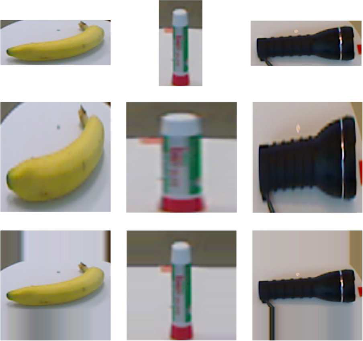
The results of image scaling. The top row shows the original images. The middle row shows the warped results, while the bottom row shows the results of using the method of Eitel et al.¹² Best viewed in colour.

The PCA–CCA network

The proposed PCA–CCA network is designed to extract features of objects using RGB and depth information jointly. Figure 3 presents a block diagram of the PCA–CCA network for RGB-D object recognition. As can be seen, the proposed method consists of two convolution layers and one output layer. Only the PCA filters in the first layer and CCA filters in the second layer need to be learned from the input RGB-D images. Further details of the processes involved are given below.

Figure 3.

The block diagram of the PCA–CCA network. PCA filters in the first convolution layer are learned using the RGB and depth images separately. $W_{1}^{c}, W_{2}^{c} ... W_{L_{1}}^{c}$ and $W_{1}^{d}, W_{2}^{d} ... W_{L_{1}}^{d}$ are the PCA filters in the first layer for RGB and depth components. Then, outputs of RGB and depth components in the first layer are fused to generate the CCA filters in the second convolution layer. $V_{1}^{c}, V_{2}^{c} ... V_{L_{2}}^{c}$ and $V_{1}^{d}, V_{2}^{d} ... V_{L_{2}}^{d}$ are the CCA filters in the second layer for RGB and depth components. Best viewed in colour. PCA: principal component analysis; CCA: canonical correlation analysis.

The first convolution layer

In the first convolution layer, we employ two groups of PCA filters for the RGB and depth components. Each group of filters are learned separately. The data input into this layer correspond to the cropped and preprocessed RGB-D images. The pseudocolour depth images can also be regarded as three-channel RGB images, so the RGB and depth components in the first layer are the same. Therefore, we will only describe the RGB component in detail for the sake of brevity.

Suppose that there are N RGB images input for training purposes which we denote by ${I_{i}^{c}}_{i = 1}^{N}$ . The image size is assumed to be m × n and the patch size k ₁ × k ₂. For each channel in the RGB images, all the patches in the i th image are collected taking an overlapping approach; that is, we have $x_{i,1}, x_{i,2},..., x_{i, m n} \in ℝ^{k_{1} k_{2}}$ where x_i,j denotes the j th vectorized patch in $I_{i}^{c}$ . Then, we subtract the patch mean from each patch to get ${\bar{X}}_{i} = [{\bar{x}}_{i,1}, {\bar{x}}_{i,2},..., {\bar{x}}_{i, m n}]$ , where ${\bar{x}}_{i, j}$ is a mean-removed patch. By constructing the similar matrix for all input images and putting them together, we get

X = [{\bar{X}}_{1}, {\bar{X}}_{2},..., {\bar{X}}_{N}] \in ℝ^{k_{1} k_{2} \times N m n}

For a given RGB image, we gather the same individual matrices for the three channels of the RGB images denoted by $X_{r}, X_{g}, X_{b} \in ℝ^{k_{1} k_{2} \times N m n}$ . Assuming that the number of filters in layer i is L_i , we use PCA to minimize the reconstruction error within a set of orthogonal filters

min_{V \in ℝ^{3 k_{1} k_{2} \times L_{1}}} {‖ \tilde{X} - V V^{T} \tilde{X} ‖}_{F}^{2}, s . t . V^{T} V = I_{L_{1}}

where $\tilde{X} = [X_{r}^{T}, X_{g}^{T}, X_{b}^{T}]$ , $I_{L_{1}}$ is the L ₁ × L ₁ identity matrix, and V is a matrix consisting of a set of eigenvectors. On solving the optimization problem, we get the L ₁ principal eigenvectors of XX^T . Then, the PCA filters of the first stage can be written as follows

W_{l}^{c} = {mat}_{k_{1}, k_{2},3} (q_{l} (\tilde{X} {\tilde{X}}^{T})) \in ℝ^{k_{1} \times k_{2} \times 3}

where $l = 1, 2, ..., L_{1}$ , $q_{l} (\tilde{X} {\tilde{X}}^{T})$ is the l th principal eigenvector of $\tilde{X} {\tilde{X}}^{T}$ , and ${mat}_{k_{1}, k_{2},3} (v)$ is a function that maps $v \in ℝ^{3 k_{1} k_{2}}$ to a matrix $W \in ℝ^{k_{1} \times k_{2} \times 3}$ . Finally, the output from the RGB component in first layer has the form

I_{i}^{c, l} = I_{i}^{c} * W_{l}^{c}, i = 1, 2, ..., N

where $I_{i}^{c}$ is the i th input RGB image, and $W_{l}^{c}$ is the l th filter of the PCA filter bank for the RGB component in the first layer.

Similarly, for the depth images that are input, the PCA filters can be denoted as $W_{l}^{d}, l = 1, 2, ..., L_{1}$ . The output from the depth component in the first layer has the form

I_{i}^{d, l} = I_{i}^{d} * W_{l}^{d}, i = 1, 2, ..., N

where $I_{i}^{d}$ is the i th input depth image, and $W_{l}^{d}$ is the l th filter of the PCA filter bank for the depth component.

The second convolution layer

The data input into this layer consists of the output from the first layer. We employ the CCA method to generate the filters for the RGB and depth components.

For the RGB or depth component, all the overlapping patches of $I_{i}^{l}$ are collected and the patch means subtracted. This yields ${\bar{Y}}_{i}^{l} = [{\bar{y}}_{i, l,1}, {\bar{y}}_{i, l,2},..., {\bar{y}}_{i, l, m n}] \in ℝ^{k_{1} k_{2} \times m n}$ , where ${\bar{y}}_{i, l, j}$ is the j th mean-removed patch in $I_{i}^{l}$ . We then define $Y^{l} = [{\bar{Y}}_{1}^{l}, {\bar{Y}}_{2}^{l},..., {\bar{Y}}_{N}^{l}] \in ℝ^{k_{1} k_{2} \times N m n}$ to be all the mean-removed patches of the l th filter output. Thus, all of the filter outputs in a single component can be expressed as follows

Y = [Y^{1}, Y^{2},..., Y^{L_{1}}] \in ℝ^{k_{1} k_{2} \times L_{1} N m n}

so that we can obtain Y_c and Y_d for the RGB and depth components, respectively.

The aim of CCA is to find projections of two sets of samples that simultaneously yield the maximum correlation. Here, the CCA filters in this layer are the projections that make the outputs of the RGB and depth components (Y_c and Y_d ) have maximal correlation. The first projection directions α ₁ and β ₁ (for colour and depth, respectively) can be obtained by solving the following optimization problem

\begin{matrix} max α_{1}^{T} Σ_{Y_{c} Y_{d}} β_{1} \\ s.t. α_{1}^{T} Σ_{Y_{c} Y_{c}} α_{1} = β_{1}^{T} Σ_{Y_{d} Y_{d}} β_{1} = 1 \end{matrix}

where $Σ_{Y_{c} Y_{c}}$ and $Σ_{Y_{d} Y_{d}}$ denote the intraclass and $Σ_{Y_{c} Y_{d}}$ and $Σ_{Y_{d} Y_{c}}$ ( $= Σ_{Y_{c} Y_{d}}$ ) the extraclass covariance matrices, respectively. Optimization can be carried out using the Lagrange multiplier technique. The optimization problem in Equation (7) is thus written in the form

\begin{matrix} L (α_{1}, β_{1}, λ) = α_{1}^{T} Σ_{Y_{c} Y_{d}} β_{1} - \frac{λ_{1}}{2} (α_{1}^{T} Σ_{Y_{c} Y_{c}} α_{1} - 1) - \\ \frac{λ_{2}}{2} (β_{1}^{T} Σ_{Y_{d} Y_{d}} β_{1} - 1) \end{matrix}

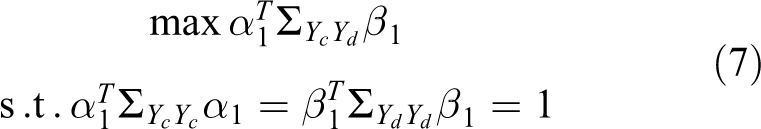
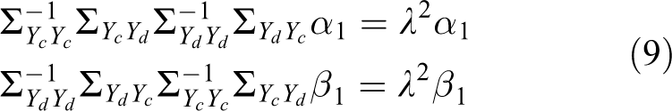
where λ ₁ and λ ₂ are Lagrange multipliers. Setting $\partial L / \partial α_{1} = 0$ and $\partial L / \partial β_{1} = 0$ , we find

\begin{array}{l} Σ_{Y_{c} Y_{c}}^{- 1} Σ_{Y_{c} Y_{d}} Σ_{Y_{d} Y_{d}}^{- 1} Σ_{Y_{d} Y_{c}} α_{1} = λ^{2} α_{1} \\ Σ_{Y_{d} Y_{d}}^{- 1} Σ_{Y_{d} Y_{c}} Σ_{Y_{c} Y_{c}}^{- 1} Σ_{Y_{c} Y_{d}} β_{1} = λ^{2} β_{1} \end{array}

where λ = λ ₁ = λ ₂. Thus, α ₁ and β ₁ are the eigenvectors of $Σ_{Y_{c} Y_{c}}^{- 1} Σ_{Y_{c} Y_{d}} Σ_{Y_{d} Y_{d}}^{- 1} Σ_{Y_{d} Y_{c}}$ and $Σ_{Y_{d} Y_{d}}^{- 1} Σ_{Y_{d} Y_{c}} Σ_{Y_{c} Y_{c}}^{- 1} Σ_{Y_{c} Y_{d}}$ , respectively, corresponding to the largest eigenvalue, λ ². Given the first ℓ − 1 directions, the ℓ th projection direction can be calculated by solving the problem in Equation (7) with the additional constraints that $α_{i}^{T} Σ_{Y_{c} Y_{c}} α_{ℓ} = β_{i}^{T} Σ_{Y_{d} Y_{d}} β_{ℓ} = 0$ (i < ℓ).

The CCA filters of the second layer can now be expressed as follows

\begin{array}{l} V_{ℓ}^{c} = {mat}_{k_{1}, k_{2}} (α_{ℓ}) \in ℝ^{k_{1} \times k_{2}} \\ V_{ℓ}^{d} = {mat}_{k_{1}, k_{2}} (β_{ℓ}) \in ℝ^{k_{1} \times k_{2}} \end{array}

where $ℓ = 1, 2, ..., L_{2}$ and ${mat}_{k_{1}, k_{2}} (α_{ℓ})$ maps the vector $α_{ℓ} \in ℝ^{k_{1} k_{2}}$ to the matrix $V_{ℓ}^{c} \in ℝ^{k_{1} \times k_{2}}$ . The matrices $V_{ℓ}^{c}$ and $V_{ℓ}^{d}$ represent the ℓ th filter of the RGB and depth components, respectively.

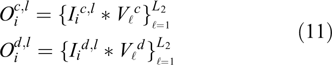
Finally, for each input $I_{i}^{l}$ of the second layer, we will have L ₂ outputs, each found by convoluting $I_{i}^{l}$ with V_ℓ for ℓ = 1, 2,..., L ₂

\begin{array}{l} O_{i}^{c, l} = {I_{i}^{c, l} * V_{ℓ}^{c}}_{_{ℓ = 1}}^{L_{2}} \\ O_{i}^{d, l} = {I_{i}^{d, l} * V_{ℓ}^{d}}_{_{ℓ = 1}}^{L_{2}} \end{array}

The total number of outputs from the second layer is therefore $2 L_{1} L_{2}$ .

The output layer

The output layer is used to generate the final feature expression of each training RGB-D image. RGB and depth components are handled separately, and the processes are the same. Hence, we will only describe the process for the RGB component for the sake of brevity, as we did before.

After the second layer, for each of the L ₁ inputs $I_{i}^{c, l}$ in the RGB component, there are L ₂ real-valued outputs ${I_{i}^{c, l} * V_{ℓ}^{c}}_{_{l = ℓ}}^{L_{2}}$ . These outputs are binarized into the form ${H (I_{i}^{c, l} * V_{ℓ}^{c})}_{_{ℓ = 1}}^{L_{2}}$ where the Heaviside function is such that the value of H(⋅) is 1 if the argument is positive, and 0 otherwise. Then, we view each corresponding pixel of the L ₂ output as L ₂ binary bits which we convert to a decimal number, $T_{i}^{c, l}$ , given by

T_{i}^{c, l} = \sum_{ℓ = 1}^{L_{2}} 2^{ℓ - 1} H (I_{i}^{c, l} * V_{ℓ}^{c})

The above process converts the L ₂ outputs in $O_{i}^{c, l}$ back into a single integer-valued ‘image’, whose every pixel is an integer in the range ${[0, 2}^{L_{2}} - 1]$ .

Now L ₁ single integer-valued ‘images’ are obtained. Each of these is partitioned into H blocks and a histogram of the decimal values in each block is computed. Finally, the H histograms are concatenated into one vector $Hist (T_{i}^{c, l}), l = 1, 2, ..., L_{1}$ . After the encoding process above, the feature of the input RGB component $I_{i}^{c}$ is defined as follows

f_{i}^{c} = [Hist (T_{i}^{c,1}),..., Hist (T_{i}^{c, L_{1}} {)]}^{T} \in ℝ^{{(2}^{L_{2}}) L_{1} H}

Similarly, the feature of the depth component is denoted as follows

f_{i}^{d} = [Hist (T_{i}^{d,1}),..., Hist (T_{i}^{d, L_{1}} {)]}^{T} \in ℝ^{{(2}^{L_{2}}) L_{1} H}

Finally, the feature of the i th input RGB-D data is $f_{i} = [f_{i}^{c} f_{i}^{d}] \in ℝ^{2 \times {(2}^{L_{2}}) L_{1} H}$ .

Experiments

The proposed method was implemented using MATLAB on a computer built around an Intel Xeon E5 CPU (8-cores operating at 2.4 GHz). To evaluate the effectiveness of the proposed PCA–CCA network, experiments were conducted on the challenging Washington RGB-D object data set.¹⁷ The details of these experiments and the results are described below.

Data set and experiment set-up

There are 300 household objects in 51 categories in the Washington RGB-D object data set. Each object was captured using a Kinect-style 3D camera which was placed at three different heights and multiple views. The object recognition experiments in this article are focused on category recognition. Therefore, the proposed PCA–CCA network method was evaluated using the same (10) cross-validation splits as used by Lai et al.¹⁷ Each split consists of roughly 35,000 training and 7000 testing images. The task of the PCA–CCA network is to correctly predict the category of a new instance.

In our experiments, the image size used was 90 × 90, the patch size was 5 × 5, the filter numbers were L ₁ = 12 and L ₂ = 8, and the block size was 4 × 4. As the object images consist of complex poses, spatial pyramid pooling³⁷ was applied to the output layer (a pyramid of 4 × 4, 2 × 2, 1 × 1 was used). The dimension of each pooled feature is reduced to 640 by the PCA process. Hence, the feature dimension of each input RGB-D image pair is $640 \times (4 \times 4 + 2 \times 2 + 1) \times 2 = 26, 880$ . The process not only extracts the information that is invariant to large changes in pose but also reduces the runtimes necessary for training of the classifier and prediction.

For classification purposes, a linear SVM was employed and the LIBLINEAR library³⁸ was used for its implementation.

Results and analysis

Comparison with different baselines

Our method is designed for RGB-D images and has a structure similar to that of PCANet. Therefore, the original PCANet method can also be applied to the RGB-D data with some common multimodal fusion approaches. Thus, we conducted six different PCANet baselines:

RGB PCANet: PCANet trained using only RGB images.

Depth PCANet: PCANet trained using only depth images.

Early-fusion PCANet: PCANet with separate training for colour and depth images, followed by concatenating the features of the colour and depth images. This method is similar to that used by Schwarz et al.²⁵ (This is actually an example of an early-fusion scheme as described by Sanchez et al.²⁹ hence the name).

Late-fusion PCANet: PCANet with separate training for colour and depth images and classifiers that are also trained separately. The final result is obtained by selecting the modality with the maximum classification score. (Named after the late-fusion scheme described by Sanchez et al.²⁹).

Early-fusion PCANet with pseudocolour depth: The same structure used in early-fusion PCANet but pseudocolour depth images is used.

Late-fusion PCANet with pseudocolour depth: The same structure used in late-fusion PCANet but pseudocolour depth images is used.

A linear SVM method is used as classifier when testing each of the six baselines.

Table 1 shows a comparison of the accuracy of the recognition results achieved using our method and the six baselines. Methods using both the RGB and depth components achieve a significantly greater accuracy compared to the RGB PCANet method. The performance of the early-fusion methods is better than that of the late-fusion methods. The pseudocolour depth images help improve the accuracy in both the early- and late-fusion methods which means that the pseudocolour information helps with the discrimination process. The best of the baseline results was achieved by the early-fusion PCANet with pseudocolour depth method (whose structure is the most similar to ours). However, our method achieves an even better result (by 2%). The reason for this is that in our method, the correlation features are extracted jointly by the CCA filters (the discriminative features learned by the PCA filters are similar to those in the early-fusion PCANet with pseudocolour depth method). This results in a more discriminative description of the features of the RGB-D data which can also eliminate redundant information at the same time.

Table 1.

Comparison of different baselines obtained using the Washington RGB-D object data set.

Method	Accuracy (%)
RGB PCANet	82.3 ± 3.4
Depth PCANet	75.6 ± 2.0
Early-fusion PCANet	88.4 ± 3.4
Late-fusion PCANet	87.6 ± 1.9
Early-fusion PCANet with pseudocolour depth	89.7 ± 2.3
Late-fusion PCANet with pseudocolour depth	89.2 ± 2.5
Ours	91.7 ± 1.4

PCA: principal component analysis. The bold values show the accuracy result of our method and the best one within other methods listed in this table.

Comparison with state-of-the-art methods

We next compared the accuracy of our proposed method with that obtained using some state-of-the-art methods (Table 2). The recognition accuracy of our method is 91.7% (on average) over the 51 categories of objects. This outperforms all of the approaches listed except for the query adaptive similarity measure (QASM) method.³² We note that QASM is a higher level ensemble method rather than a classification method. Our method and the other methods in Table 2 (except QASM) are essentially classification methods. More specifically, the whole process of QASM consists of two steps. In the first step, an object classification method is used to obtain the classification scores, and in the second step, the similarity measurement method is conducted using the output scores. In the article of QASM,³² the CNN–RNN method was used in the first step. A comparison of runtime costs is presented in Table 3, which indicates that our method is more efficient than the CNN-RNN method. (The runtimes shown in Table 3 are discussed in greater detail later on in this article.) CNN–RNN method is more efficient than QASM method, so our method is also more efficient than QASM. Moreover, QASM is not specifically designed for CNN–RNN and can also be used with other object classification methods, including ours. In future application, therefore, we may, in principle, be able to achieve an even better accuracy using their ensemble mechanism.

Table 2.

Comparison with other approaches reported for the Washington RGB-D object data set.

Method	Accuracy (%)
Nonlinear SVM¹⁷ (2011)	83.9 ± 3.5
KDES¹⁸ (2011)	86.2 ± 2.1
Upgraded HMP² (2013)	87.5 ± 2.9
CKM²² (2012)	86.4 ± 2.3
CNN-RNN²⁴ (2012)	86.8 ± 3.3
LMMM²⁸ (2015)	86.9 ± 2.6
CNN features²⁵ (2015)	89.4 ± 1.3
Fus-CNN¹² (2015)	91.3 ± 1.4
CFK²⁷ (2015)	91.2 ± 1.5
Hypercube pyramid³⁰ (2016)	91.1 ± 1.4
QASM³² (2015)	92.7 ± 1.0
Ours	91.7 ± 1.4

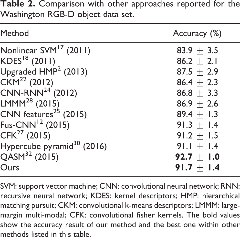
SVM: support vector machine; CNN: convolutional neural network; RNN: recursive neural network; KDES: kernel descriptors; HMP: hierarchical matching pursuit; CKM: convolutional k-means descriptors; LMMM: large-margin multi-modal; CFK: convolutional fisher kernels. The bold values show the accuracy result of our method and the best one within other methods listed in this table.

Table 3.

A comparison of runtime costs.^a

Method	Runtime (s)
CKM²² (2012)	1.13
CNN–RNN²⁴ (2012)	1.01
Upgraded HMP²¹ (2013)	1.22
Fus-CNN¹² (2015)	0.46
Early-fusion PCANet with pseudocolour depth	0.43
Ours	0.44

PCA: principal component analysis; CNN: convolutional neural network; RNN: recursive neural network. The bold values show the runtime result of our method and the best one within other methods listed in this table.

^aThe times include all preprocessing steps and were achieved using a computer powered by an Intel Xeon E5 2.4 GHz CPU (no GPU was used).

The more recently developed CNN-based methods generally have a complex network structure. For example, Schwarz et al.²⁵ (CNN Features) and Fus-CNN¹² used CNNs with eight layers. Zaki et al.³⁰ (hypercube pyramid) employed a network with six layers and proposed the use of a hypercube pyramid scheme. However, in our method, there are only two convolution layers and an output layer which is clearly a simpler approach. In addition, Schwarz et al.²⁵ (CNN Features) extracted the features of the RGB and depth images separately whereas, in our method, the correlation between RGB and depth is considered which gives a better performance.

One of the benefits of the simplicity of the structure used in our method is that there are few parameters to be tuned when training the network (patch size, number of filters and block size of the histograms). The parameters that need to be fine-tuned in CNN-based methods include the network weights and biases and the hyperparameters (these include learning rate, batch size, number of epoch, number of kernels, kernel size and pooling size). The hyperparameters are tuned manually while the weights and biases are tuned iteratively using back-propagation until convergence is achieved. This process is very time-consuming because there are numerous weight parameters to be tuned. Therefore, the training in CNN-based methods generally uses GPUs to accelerate the process. For example, the training of a single network took 10 h using an NVIDIA 790 GPU in the work by Eitel et al.¹² and a training time of 4.5 h is reported by Wang et al.²⁸ using a Titan GPU. In our method, only PCA and CCA filters need to be learned directly and there is no need to iteratively tune weights. Moreover, the hyperparameters in our method are few in number. As a result, it only takes 1.5 h to train our network using a CPU-only platform.

Parameter analysis

The images in the Washington RGB-D object data set had to be scaled using the previously mentioned scaling approach in order to satisfy the requirements of the PCA–CCA network. The image size was set to 90 × 90 (as most of the original images in the data set are around this size). If the scaled image is much smaller than the original, then some local information may be lost which is a very important issue if classification is to be accurate. Moreover, using a size larger than 90 cannot yield a higher accuracy in our experiments, but it will increase the feature extraction runtime significantly.

The model parameters in the PCA–CCA network that affect classification performance are patch size and filter number. To show the effect of using different patch sizes, we fixed the filter numbers (with L ₁ = 12 and L ₂ = 8) and varied the patch size from 3 × 3 to 9 × 9. The results are shown in Figure 4. The best accuracy appears to occur when the patch size is 5 × 5. When the patch size exceeds 5 × 5, the accuracy decreases significantly. This is because larger sized patches cannot capture enough local information, which is of vital importance in describing the objects.

Figure 4.

Recognition accuracy of the PCA–CCA network as a function of patch size (L ₁ = 12 and L ₂ = 8). PCA: principal component analysis; CCA: canonical correlation analysis.

To investigate the effect of changing the number of filters, we varied the PCA filter number L ₁ from 8 to 14, keeping the other quantity fixed with L ₂ = 8 (Figure 5). Clearly, accuracy tends to increase as L ₁ becomes larger. When L ₁ > 12, however, the accuracy drops off to some extent. This is because some redundant information may be included in the final feature representation. Note that using more filters will dramatically increase runtime and memory usage. Hence, L ₁ was set to 12 to obtain good results while keeping the computational burden bearable.

Figure 5.

Recognition accuracy of the PCA–CCA network as a function of PCA filter number (L ₂ = 8). PCA: principal component analysis; CCA: canonical correlation analysis.

Next, the number of CCA filters L ₂ was varied from 6 to 12, keeping L ₁ fixed at 12 (Figure 6). We can see that, in this case, the best accuracy occurs when L ₂ = 8 and that increasing L ₂ further only reduces performance.

Figure 6.

Recognition accuracy of the PCA–CCA network as a function of CCA filter number (L ₁ = 12). PCA: principal component analysis; CCA: canonical correlation analysis.

Error analysis

Figure 7 shows the confusion matrix of the recognition results obtained using the proposed method applied to the Washington RGB-D data set. As can be seen, most categories can be classified correctly, which demonstrates the effectiveness of the proposed method. However, there are some categories which are often misclassified, for example, pitcher, mushroom, peach and food jar (Figure 8). These misclassifications occur because some instances share similar colours and shapes with other instances in different categories. In addition, there are only a very small number of training samples for the category mushroom and great differences between instances. These categories may be very difficult to recognize correctly, even for humans.

Figure 7.

Confusion matrix of the proposed method on Washington RGB-D data set. The y-axis shows the true labels of the testing objects, and the x-axis shows the predicted labels. Best viewed in colour.

Figure 8.

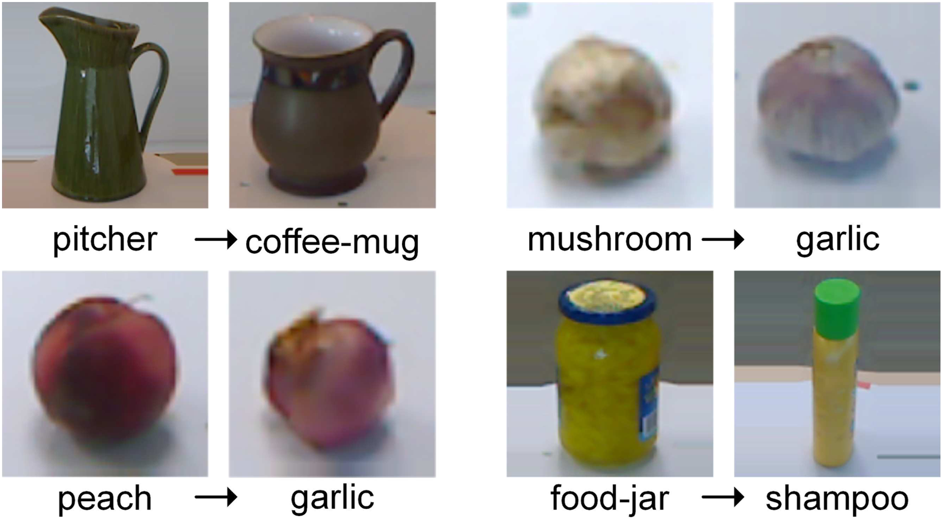
Examples of some easily misclassified categories. Misclassification occurs due to the strong similarities in the objects’ colours and shapes.

Running time

Computing power is usually very constrained in mobile robotic applications. We tested the average runtime of different feature extraction and prediction procedures using the Washington RGB-D object data set. Our method required 0.44 s per input object which is low enough to allow frame rates of about 2.3 Hz. We also made a runtime cost comparison with state-of-the-art methods whose source codes are available. The results are shown in Table 3 and indicate that our method and baseline method are more efficient than those used in other methods. Comparing our baseline method with the early-fusion PCANet with pseudocolour depth method, it is apparent that both methods have nearly identical runtimes. However, the accuracy of our method is better because of the special structure designed for the RGB-D data.

CNN-based methods can usually achieve a high execution efficiency provided GPUs are available. Schwarz et al.²⁵, for instance, presented feature extraction runtimes achieved using a computer equipped with an Intel Core i7 CPU chipset running at 2.7 GHz and an NVidia GeForce GT 730 M GPU. On their experimental platform, the method proposed by Bo et al.²¹ took 1.153 s to process one frame, while the CNN-based method used by Schwarz et al.²⁵ took only 0.186 s. As expected, the runtime achieved by this CNN-based method is low because of the help provided by the GPU. However, in many lightweight mobile robot applications (such as the unmanned aerial vehicle), the presence of a GPU may be undesirable when considering the limitation of energy consumption, weight, size and so on. Our method is highly efficient and accurate, even when it is just the CPU performing all the calculations. This suggests that our proposed method is ideal for use in lightweight mobile robots. We expect that our method can also be parallelized and accelerated by the use of extra GPUs (to accelerate, e.g. the convolution processes involved in the first and second layers). Thus enhanced, an optimized implementation of our method should be able to provide RGB-D object recognition in real time.

Conclusions

In this article, we propose a PCA–CCA network method for effective RGB-D object recognition. The proposed deep learning method is a simple one which considers, in addition to the discriminative characteristics of the RGB and depth modalities, the characteristics of the correlation between the two modalities. The PCA–CCA network method is composed of two convolution layer stages, binary hashing and block-wise histograms. In the first layer, PCA filters are applied to the RGB and depth components separately. Then, the CCA filters are learned using both of the two components together.

Experiments were conducted on the Washington RGB-D object data set which demonstrate that our method has an accuracy that is comparable to state-of-the-art methods. In addition, as our method has a simple structure, it is efficient even without GPU acceleration. In future work, we intend to focus on a more robust approach that can deal with occlusion between objects. We also aim to perform more experiments on real scenes.

Footnotes

Declaration of conflicting interests

The author(s) declared no potential conflict of interest with respect to the research, authorship and/or publication of this article.

Funding

The author(s) disclosed receipt of the following financial support for the research, authorship and/or publication of this article: This work was supported by the National Natural Science Foundation of China under grant (61673378, 61421004) and was supported in part by the basic research program under grant B132011.

References

Swain

Ballard

. Color indexing. Int J Comput Vision 1991; 7(1): 11–32.

Lowe

. Object recognition from local scale-invariant features. In: The proceedings of the seventh IEEE international conference on computer vision 1999, Kerkyra, Greece, 20–27 September 1999, vol. 2, pp. 1150–1157. IEEE.

Bay

Ess

Tuytelaars

. Speeded-up robust features (surf). Comput Vision Image Understand 2008; 110(3): 346–359.

Krizhevsky

Sutskever

Hinton

. Imagenet classification with deep convolutional neural networks. In: Advances in neural information processing systems, Stateline, United States, 3–8 December 2012, pp. 1097–1105.

Farabet

Couprie

Najman

. Learning hierarchical features for scene labeling. IEEE Trans Pattern Anal Mach Int 2013; 35(8): 1915–1929.

Oquab

Bottou

Laptev

. Learning and transferring mid-level image representations using convolutional neural networks. In: Proceedings of the IEEE conference on computer vision and pattern recognition, Columbus, OH, United States, 23–28 June 2014, pp. 1717–1724.

Girshick

Donahue

Darrell

. Rich feature hierarchies for accurate object detection and semantic segmentation. In: Proceedings of the IEEE conference on computer vision and pattern recognition, Columbus, OH, United States, 23–28 June 2014, pp. 580–587.

Szegedy

Liu

Jia

. Going deeper with convolutions. In: Proceedings of the IEEE conference on computer vision and pattern recognition, Boston, MA, United States, 7–12 June 2015, pp. 1–9.

Chan

Jia

Gao

. Pcanet: a simple deep learning baseline for image classification? IEEE Trans Image Proc 2015; 24(12): 5017–5032.

10.

Jolliffe

IT.

Principal component analysis and factor analysis. In: Principal component analysis. New York: Springer, 1986, pp. 115–128.

11.

Wang

Cai

. Mmss: multi-modal sharable and specific feature learning for RGB-D object recognition. In: Proceedings of the IEEE international conference on computer vision, Santiago, Chile, 7–13 December 2015, pp. 1125–1133.

12.

Eitel

Springenberg

Spinello

. Multimodal deep learning for robust RGB-D object recognition. In: 2015 IEEE/RSJ international conference on intelligent robots and systems (IROS), Hamburg, Germany, 28 September–2 October 2015, pp. 681–687. IEEE.

13.

Hardoon

Szedmak

Shawe-Taylor

. Canonical correlation analysis: an overview with application to learning methods. Neural Comput 2004; 16(12): 2639–2664.

14.

Rusu

Blodow

Marton

. Aligning point cloud views using persistent feature histograms. In: IROS 2008. IEEE/RSJ international conference on intelligent robots and systems, Nice, France, 22–26 September 2008, pp. 3384–3391. IEEE.

15.

Rusu

Blodow

Beetz

. Fast point feature histograms (FPFH) for 3D registration. In: 2009 IEEE international conference on robotics and automation, Kobe, Japan, 12–17 May 2009, pp. 3212–3217. IEEE.

16.

Rusu

Bradski

Thibaux

. Fast 3D recognition and pose using the viewpoint feature histogram. In: 2010 IEEE/RSJ international conference on intelligent robots and systems (IROS), Taipei, Taiwan, 18–22 October 2010, pp. 2155–2162. IEEE.

17.

Lai

Liefeng

Xiaofeng

. A large-scale hierarchical multi-view RGB-D object dataset. In: 2011 IEEE international conference on robotics and automation (ICRA), Shanghai, China, 9–13 May 2011, pp. 1817–1824. IEEE.

18.

Ren

Fox

. Depth kernel descriptors for object recognition. In: 2011 IEEE/RSJ international conference on intelligent robots and systems (IROS), San Francisco, CA, USA, 25–30 September 2011, pp. 821–826. IEEE.

19.

Browatzki

Fischer

Graf

. Going into depth: Evaluating 2D and 3D cues for object classification on a new, large-scale object dataset. In: 2011 IEEE international conference on computer vision workshops (ICCV workshops), Barcelona, Spain, 6–13 November 2011, pp. 1189–1195. IEEE.

20.

Berker Logoglu

Kalkan

Temizel

. Cospair: colored histograms of spatial concentric surflet-pairs for 3D object recognition. Robot Auton Syst 2016; 75(Part B): 558–570.

21.

Ren

Fox

. Unsupervised feature learning for RGB-D based object recognition. In: Proceedings of international symposium on experimental robotics (ISER), Québec, Canada, 17–21 June 2012, pp. 387–402.

22.

Blum

Springenberg

Wulfing

. A learned feature descriptor for object recognition in RGB-D data. In: 2012 IEEE international conference on robotics and automation (ICRA), Saint Paul, MN, USA, 14–18 May 2012, pp. 1298–1303. IEEE.

23.

Asif

Bennamoun

Sohel

. Discriminative feature learning for efficient RGB-D object recognition. In: 2015 IEEE/RSJ international conference on intelligent robots and systems (IROS), Hamburg, Germany, 28 September–2 October 2015, pp. 272–279. IEEE.

24.

Socher

Huval

Bath

. Convolutional-recursive deep learning for 3D object classification. In: NIPS, Stateline, United States, 3–8 December 2012, pp. 656–664.

25.

Schwarz

Schulz

Behnke

. RGB-D object recognition and pose estimation based on pre-trained convolutional neural network features. In: 2015 IEEE international conference on robotics and automation (ICRA), Seattle, WA, USA, 26–30 May 2015, pp. 1329–1335. IEEE.

26.

Bai

Zhang

. Subset based deep learning for RGB-D object recognition. Neurocomputing 2015; 165: 280–292.

27.

Cheng

Cai

Zhao

. Convolutional fisher kernels for RGB-D object recognition. In: 2015 international conference on 3D vision (3DV), Lyon, France, 19–22 October 2015, pp. 135–143. IEEE.

28.

Wang

Cai

. Large-margin multi-modal deep learning for RGB-D object recognition. IEEE Trans Multimed 2015; 17(11): 1887–1898.

29.

Sanchez-Riera

Hua

Hsiao

. A comparative study of data fusion for RGB-D based visual recognition. Pattern Recognit Lett 2016; 73: 1–6.

30.

Zaki

Shafait

Mian

. Convolutional hypercube pyramid for accurate RGB-D object category and instance recognition. In: 2016 IEEE international conference on robotics and automation (ICRA), Stockholm, Sweden, 16–21 May 2016, pp. 1685–1692. IEEE.

31.

Zaki

Shafait

Mian

. Learning a deeply supervised multi-modal RGB-D embedding for semantic scene and object category recognition. Robot Auton Syst 2017; 92: 41–52.

32.

Cheng

Cai

Zhang

. Query adaptive similarity measure for RGB-D object recognition. In: Proceedings of the IEEE international conference on computer vision, Santiago, Chile, 7–13 December 2015, pp. 145–153. IEEE.

33.

Tian

Fan

Ming

. Stacked PCA network (spcanet): an effective deep learning for face recognition. In: 2015 IEEE international conference on digital signal processing (DSP), Singapore, 21–24 July 2015, pp. 1039–1043. IEEE.

34.

Jia

Han

Gao

. 2dpcanet: Dayside aurora classification based on deep learning. In: CCF Chinese conference on computer vision, Xi’an, China, 18–20 September 2015, pp. 323–334. Springer.

35.

Huang

Yuan

. Weighted-PCAnet for face recognition. In: International conference on neural information processing, Istanbul, Turkey, 9–12 November 2015, pp. 246–254. Springer.

36.

Zeng

Shao

. Color image classification via quaternion principal component analysis network. Neurocomputing 2016; 216: 416–428.

37.

Zhang

Ren

. Spatial pyramid pooling in deep convolutional networks for visual recognition. In: European conference on computer vision, Zurich, Switzerland, 6–12 September 2014, pp. 346–361. Springer.

38.

Fan

Chang

Hsieh

. Liblinear: a library for large linear classification. J Mach Learn Res 2008; 9: 1871–1874.

A PCA–CCA network for RGB-D object recognition

Abstract

Keywords

Introduction

Related work

RGB-D image preprocessing

Encoding the raw depth images

Image scaling

The PCA–CCA network

The first convolution layer

The second convolution layer

The output layer

Experiments

Data set and experiment set-up

Results and analysis

Comparison with different baselines

Comparison with state-of-the-art methods

Parameter analysis

Error analysis

Running time

Conclusions

Footnotes

Declaration of conflicting interests

Funding

References